A Mixed Method for Feature Extraction Based on Resonance Filtering

1  Introduction

Image-based machine learning tasks requires neural networks to select features that can identify images well. Some scholars are devoted to the study of image feature extraction [1,2]. Feature extraction can be used for image classification [3,4], image segmentation [4–7], target detection [8–11], attention mechanism of the visual system [11–16] and other research directions. Images have individual features and common features, which are adversarial and interdependent in image recognition. Overemphasizing individual or common features can make neural network training problematic. How to analyze the individual characteristics and common characteristics of images and use them reasonably is the key to solving the problem. After the image is rotated and stretched, the neural network can still learn the patterns in the data, and the noise of the image will damage the training of the neural network.

There is still room for improvement in the accuracy of neural network feature extraction. In this paper, resonance filtering is used to filter noise to improve the feature extraction accuracy of neural network. Resonance filtering uses the resonance process to suppress the detuned signal by simulating a series resonant circuit to filter noise data. Put the resonance layer on the input layer of the neural network, turn off the output of the neuron whose error is difficult to reduce during training, and filter the “detuned signal” in the input data to achieve the effect of filtering noise. Resonance filtering is an electrical concept, which is rarely used in neural network structure. In this paper, frequency parameters are introduced using resonance filtering, which simulates the sensitivity of neurons to data features and extracts common features of images in the form of filtering.

The individual characteristics of the image can be realized by some image processing algorithms such as skeleton extraction and edge detection. The classic K3M skeleton extraction algorithm [17] belongs to a type of iterative boundary erosion algorithm. The algorithm uses contours to corrode the boundary of the target image, gradually refines the target and extracts the skeleton. The symbolic images extracted by the skeleton often conform to human understanding of structural features, reflect a highly concentrated state, and have a high guiding significance for neural network training. Edge detection is usually in the initial stage of image processing, and its reliability will directly affect the system’s understanding of objective reality. Generally speaking, the boundary of the image is usually approximately equal to the boundary of the feature distribution, such as Canny operator [18], PiDiNet [19], BDCN [20], edge detection method for infrared image [21], semantic edge detection [22] and so on.

In order to better fuse individual features and remove image noise, this paper designs a resonance-based feature extraction method. The position of the resonance layer is before the input layer, and the mixed method mentioned in this paper will use the skeleton extracted by K3M, the boundary extracted by the Canny algorithm, and the image filtered by the resonance filter to reconstruct the training image. The purpose of the resonance layer is to improve the feature extraction efficiency of the neural network by efficiently expressing the common and individual characteristics of the training set images, thereby improving the accuracy of neural network prediction. The National Institute of Standards and Technology constructed binary images of handwritten digits database, which is called MNIST. Using the handwritten digital image database, experiments on the structure of the fully connected neural network(FNN) and LeNet-5 [23] neural network show that the mixed feature extraction method consisting of skeleton, edge and resonance filtering improves the accuracy of training.

2  Resonance Filtering

In this paper, due to the ability of the resonant layer to suppress detuned signals, the resonance layer can monitor the error of the input layer and manage the input, indirectly participating in the neural network inference process. Resonance layer using a mathematical model (see Eq. (1)) of the series resonant circuit. The practical use of this kind of resonant circuit is mostly the filtering of electrical signals, and this paper will use its mathematical model for the construction of the feature extraction algorithm.

II0=11+Q2(ωω0−ω0ω)2 (1)

2.1 Resonance Simulation

The cerebral cortex visual field is composed of simple cells and complex cells, which fire in response to properties of strip or edge-shaped visual sensory inputs [24]. The vision system contains a large number of feature detectors edges and stripes of various widths and directions. This type of discovery or theory provides a realistic basis and reference for the subsequent artificial neural network design. The visual information is processed in parallel by many independent directions and spatial-frequency-tuned modules, which presents a completely different perspective. On the premise of affirming the importance of neural linear operation mechanism, the linear theory cannot fully explain the visual system. Our ability to perceive the details of the visual scene is determined by the comparison between the relative size and the current details. Linear theory may not be able to explain the contrast sensitivity of the visual nerve. This is an inspiration of this paper to try to pretreat features by introducing input frequencies. The resonance layer realizes the filtering effect of the input data.

Firstly, the input data is regarded as a current, and the data of each channel is the component of this current, so as to introduce the frequency characteristics of the input data. Secondly, the neural network is regarded as a critically stable state. In this state, the environment will force it to be in a hypothetical natural vibration state. Any disturbance will destabilize this vibration, however the environment will eventually return the vibration to its natural state. The frequency of this natural vibration is called the ambient frequency of the resonance layer. This method uses a series resonant circuit to limit the circuit current, and it establishes a filtering mechanism that enables the neural network to use the resonance layer to suppress the input of “detuned data”. At the same time, the original image data is simulated as the effective value of “current”, see Eq. (2).

xjl=22Ajl (2)

Xjl=Ajlcos⁡(ω0jltjl+φjl)+pjl (3)

In Eqs. (2) and (3), where the superscript l represents the neural network layer l, the subscript j represents the j neuron in this layer. In Eq. (2), x is the input data, A is the resonance coefficient. In Eq. (3), it is assumed that the input data is a wave signal, X is the waveform function of input data x, A is the resonance coefficient, ω0 is the input frequency, and t is the independent variable of the wave function, φ is the phase of the wave function, and p is the offset of the wave function.

G(ω0,ω)=11+Q2(ωω0−ω0ω)2 (4)

v=G(ω0,ω) (5)

Imitate the functional relationship of the series resonance circuit (Eq. (1)) to construct Eq. (4), where ω0 is the input frequency, ω is the ambient frequency of the resonance layer, Q is the quality factor. v is the resonance coefficient. It represents the effect on the amplitude when two waves of different frequencies interact. There is a hyper-parameter in the training process of the resonance layer—quality factor Q (the name is derived from the parameter name of the AC resonance circuit), and the frequency selection range of the resonance layer can be adjusted by adjusting the quality factor.

z0=F(v,x) (6)

The v in Eq. (6) follows Eq. (5), where z0 represents the input data of the input layer. The whole process simulates the resonance process of the resonance circuit. ( ⊗ represents matrix elements corresponding to multiplication)

The symbol ⊗ represents the multiplication of the corresponding elements of the matrix. Examples are as follows in Eq. (7):

[2368]⊗[4795]=[8215440] (7)

2.2 Multi-Channel Pre-Training

Set the resonance layer before the input layer. During the training process, the resonance layer will evaluate and filter the data points of the input layer, and then input the filtered data into the neural network. As shown in Fig. 1, there is a 1-to-1 correspondence between the resonance layer and the input layer. In this method, a resonance layer vn is established for each type of data Dn, and the size and shape of the resonance layer are the same as the input layer.

F(v,x)=kf⊗(v⊗x)+bf (8)

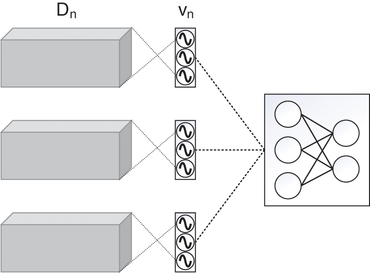
Figure 1: Structure diagram of resonance layer

Eq. (8) F(⋅) is a linear function, kf is the filter coefficient, and bf is the filter bias. The data after resonance filtering is finally input into the neural network input layer through F(⋅) .

2.3 Training Method of Resonance Network

In the training of the resonance layer, the input frequency ω0 is initialized to 0, and the environmental frequency ω of the resonance layer is initialized to 1. In the training of the resonance neural network, the resonance layer and the neural network can be trained asynchronously, or the pre-trained resonance layer can be directly used in the neural network training.

Cost=12‖y−aL‖2 (9)

al=σ(zl) (10)

δl=∂Cost∂zl (11)

δL=(aL−y)⊗σ′(zL) (12)

δl=((wl+1)Tδl+1)⊗σ′(zl) (13)

There are many superscripts in Eqs. (9)∼(13), The superscript T represents the matrix transposition. where the superscript l represents the neural network layer l( l=0,1,2… ). It should be noted that the superscript L is the maximum value of l. Eqs. (9)∼(13) and (17) are used in the traditional neural network backpropagation algorithm. For detailed derivation, please refer to the literature [25]. This section only lists the meaning of related parameters. δL is the error of the output layer, δl is the error of l layers, where the superscript L refers to the output layer, the superscript l represents the layer l, Cost is the loss, zl represents the input data of the l layer, zL represents the output layer Input data, σ(⋅) represents the activation function, al represents the activated output of the layer l, aL represents the activated output of the output layer, wl represents the weight between the l and l+1 layers, and LR is the neural network learning rate. In the actual training process, the loss function Eq. (9) can be modified according to the training situation. Unlike the classic backpropagation, the input layer error calculation formula is changed to Eq. (14) in the resonance layer training, and the update of the input frequency ω0 refers to Eq. (15).

δ0=((w1)Tδ1)⊗x (14)

In Eq. (14), δ0 is the input layer error, and x is the original input data. In training, the resonance layer uses the input layer error as the basis for tuning parameters of the resonance layer. When the error of the input layer data point in a certain period cannot be reduced, the resonance layer will filter the data point.

ω0→ω0−RLR×δ0×∂δ0δω (15)

ω0→ω0−RLR(−x⊗δ0⊗(ω/ω0−ω0/ω)−(1/ω0+ω0/ω2)(1+(ω/ω0−ω0/ω)2)32) (16)

wl=wl−LR×δl×∂δl∂wl (17)

In Eqs. (15) and (16), RLR is the learning rate of the resonance layer. In Eq. (17), wl is the weight between layer l and l + 1, and LR is the neural network learning rate. Eq. (15) uses the gradient of the error with respect to the ambient frequency of the resonance layer to update the input frequency. This parameter ω is not updated in the training process described in this paper, but it remains a variable as ambient frequency rather than a hyperparameter.

The symbol / in the Eq. (16) represents the division of the corresponding elements of the matrix. Examples are as follows in Eq. (18) :

[2368]/[4795]=[12372385] (18)

Since the resonance coefficient v is positively correlated with |ω0−ω| , the resonance process controls the sensitivity of the neuron to the data in the form of filtering, which is finally reflected in a numerical threshold-like suppression effect. The result is similar to a general adaptive filter. For data that cannot be learned, the parameter changes caused by it are “disordered” relative to the entire learning process. The disorderly changes of the resonance layer parameters will cause the resonance layer to close the input of the pixel. This method is helpful to the continuous task learning in neural network. At the same time, the method of processing image occlusion [26–28] can reduce the impact of data loss on neural network training.

3  Input Image Reconstruction

This chapter attempts to use image processing results such as image edges and skeletons as the basis for image reconstruction and to bring the reconstructed image into neural network training. Among them, the generation of P3 in Section 3.3 is related to the training process, so the process of reconstructing the image can be regarded as a simple feedback system for neural network training, training data generation and input. The flowchart of the related process can be seen in Fig. 6.

3.1 Edge Detection

The edge of the image is one of the most basic shape features of the image, and it appears as a sudden change of gray and color on the pixel image. At the same time, the intensity change of the image is caused by surface discontinuities or reflectance or illumination boundaries, which all have spatial locality, so the derivation based on this is very important. Canny operator maintains the accuracy and convenience of second-order differential edge detection, and solves the problem that the second-order differential loses edge direction information at the same time. Therefore, as shown in Fig. 2, this paper will use the Canny algorithm to perform edge detection on the input image and take the edge of the image as the basis for image reconstruction.

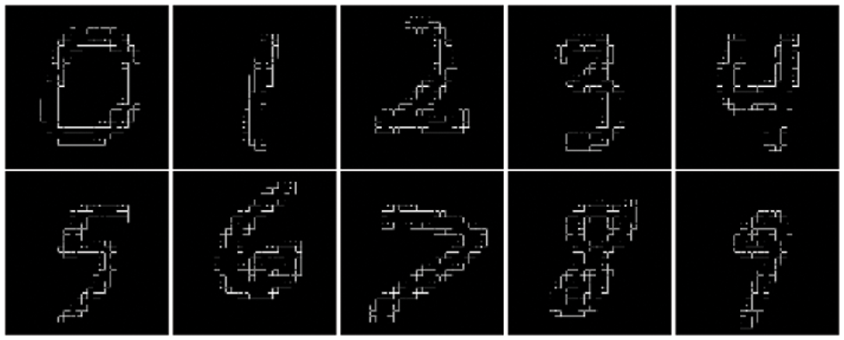
Figure 2: Example of edge detection

3.2 Keleton Extraction

The skeleton of the image can be considered as a product of image thinning. Compared with complex images, symbol images are more suitable for using this type of algorithm. This paper uses the K3M algorithm to extract the skeleton of the input image, as shown in Fig. 3, and uses the image skeleton as the basis for image reconstruction.

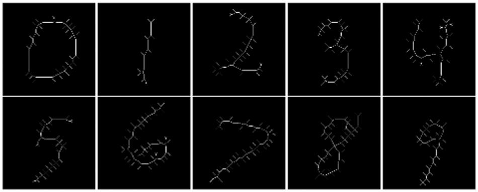
Figure 3: Example of skeleton extraction

3.3 Reconstruction of Training Images

The reconstructed image is only composed of image edges, image skeletons, and image data after resonance filtering. Variables RP (In Eq. (19)), P1, P2 and P3 represent the recombined image, the edge of the image, the image skeleton, and the image after resonance filtering respectively. As shown in Fig. 4, the reconstructed image matrix is the result of the direct addition of the three images. The edge detection calibrates the image boundary, the image skeleton represents the image frame, and the resonance filters out the common features. The reconstructed image will imply the “reasoning trend” of the artificial neural network corresponding to the original image. The essence of this trend is the derivation of the same common features. We believes that this kind of homology is the inherent requirement of the learning method based on characteristics. This method will help the neural network learn image features more three-dimensionally and vividly, and cope with more complex learning environments.

RP=P1+P2+P3 (19)

Figure 4: Example of image reconstruction

4  Training Based on Reconstructed Images

As shown in Fig. 5, the reconstructed image data is composed of the image edge, the image skeleton and the image data after resonance filtering. The resonance layer participates in the back propagation process of the neural network. The filtering result is the common feature distribution of the neural network cognition which changes with neural network training Inputting the reconstructed image of “common features + image edges + image skeleton” into the neural network will help the neural network to learn common and individual characteristics.

Figure 5: Neural network structure based on image reconstruction

Fig. 6 is a flowchart of neural network training using image reconstruction. As shown in the Fig. 6, the input image data is first processed, and then image edges, resonance filtering, and image skeleton image reconstruction are used. The reconstruction of the image is the superposition of the image edge, resonance filter, and image skeleton. In particular, resonance filter takes part in the parameter update of neural network. Finally, the neural network is input for training, and the original training process of the neural network is not affected. It should be noted that since the entire training system adds a feedback step in the input data part, the neural network will have higher robustness when faced with incorrect data input. On this basis, refer to Eq. (14) to incorporate the resonance layer parameters into the neural network parameter update system. At the same time, in order to prevent the resonance coefficient of the resonance layer from becoming all zero under extreme conditions and falling into an infinite loop that cannot be updated, the resonance layer will be derived from the input layer error to update the resonance layer as shown in Eqs. (14) and (15).

Figure 6: Training flowchart of neural network based on image reconstruction

5  Experimental Analysis

The experimental analysis is divided into three sections. Section 5.1 is the impact of using only the resonance layer to extract common features on the training of fully connected neural networks. In Section 5.2, the reconstructed image of “common feature + image edge + image skeleton” is used as the training set to train the fully connected neural network. In Section 5.3, the reconstructed image of “common feature + image edge + image skeleton” is used as the training set to train the convolutional neural network.

5.1 Resonance Filtering on the Training of FNN

This section shows the performance of neural networks and neural networks using resonance layers under the MNIST database. (add “-Re” at the end of the name to distinguish neural networks that use resonance layers). FNN stands for fully connected feed forward neural network. The fully connected neural network uses the structure of 784-200-10. In the experiment process of this section, the resonance layer is updated synchronously with the training of the neural network. Multi-channel input is used to train the resonance layer. The phase of the input data is 0, the wave function offset is 0, and the resonance coefficient is 1. For the initialization method of the frequency parameters in the neural network and the input data, see Section 1.3. The neural network learning rate LR is 0.08, and the resonance layer learning rate RLR is 0.1. There are a total of 10 epochs of training. A generation is a complete training round of the training set. The number of training rounds and the number of training generations below are synonymous.

In Fig. 7, three pictures of “original data + resonance coefficient + filtered data” from left to right are grouped together to show the data before and after filtering and the coefficient of the resonance layer.

Figure 7: Example of resonance filtering

Fig. 8 shows the accuracy of the training set of the fully connected network and the resonance network with different quality factors, which are divided into ten training rounds. From the line graph, it can be seen whether the use of resonance filtering affects the accuracy of the neural network training set. It can be seen from Fig. 8 that the convergence speed of the fully connected neural network using resonance filtering in the training set is lower than that of the neural network without resonance filtering, but the accuracy of the fully connected neural network with resonance filtering is slightly higher than that of the neural network without resonance filtering.

Figure 8: Accuracy of FNN and FNN-Re with different quality factors in the train set

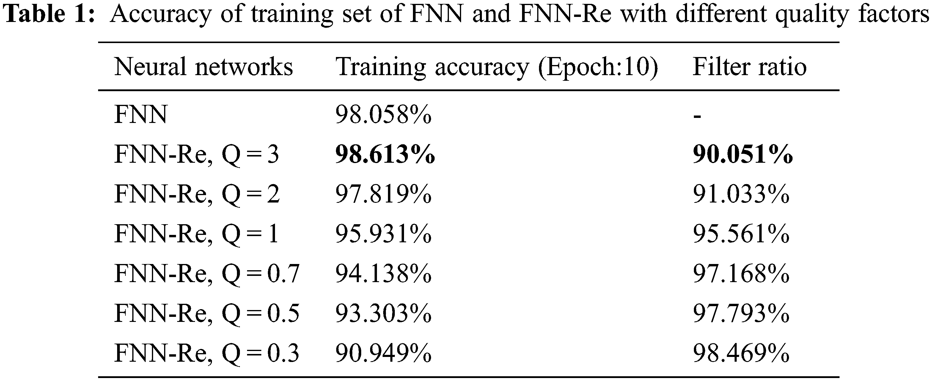
Tab. 1 shows the accuracy and filtering conditions of the neural network using resonance filtering. The “filter ratio” is the ratio of the number of pixels in the training set that changes the resonance layer to the number of pixels in the training set. The resonance layer has a small visual change to the image, but from the data in Tab. 1, the resonance layer has a huge change to the image data. We can only be sure that this change is beneficial to the accuracy of neural network training.

In general, the role of common characteristics should be emphasized. Due to the update mechanism of the neural network, the neural network will automatically learn the features that it has not learned. This mechanism is generally a learning method based on data statistics. On the one hand, less obvious features are difficult to learn. On the other hand, macroscopically, the data of a certain label and the data of other labels are confrontational and balanced. When the balance of training set diversity is broken, the damage to the model caused by input disturbances will be difficult to reverse. Therefore, the limited selection of input data based on common features will improve the stability of the neural network in the face of erroneous data.

Fig. 9 shows the training situation of the resonance layer when the quality factor is 1. From left to right, there are 10 training rounds, and from top to bottom, there are 10 categories. This figure shows the resonance layer training situation in the 10 training rounds. (the number of training rounds represents the number of times the training set has been completely trained). As the number of training rounds increases, the resonance coefficient of the resonance layer has obvious binarization and shape characteristics, and the distribution law of resonance coefficient becomes more and more clear with the training process of neural network.

Figure 9: Display of resonance coefficients

Fig. 10 shows the distribution of the resonance coefficients of the resonance layer after 10 rounds of training under different quality factors from left to right. As the quality factor decreases, the resonance coefficient distribution becomes more sparse. By controlling the size of the quality factor, the sparsity of the resonance coefficient can be controlled. In the resonant circuit, when the quality factor Q is larger, the resonant circuit’s ability to suppress detuning signals is stronger, and the circuit selectivity is better. It can be seen from Fig. 10 that when the quality factor Q becomes larger and the selectivity of the resonance layer increases, the distribution characteristics of the resonance coefficient become more obvious. From Figs. 9 and 10, the sparseness of the distribution of resonance coefficients is controlled by the number of training rounds and the quality factor.

Figure 10: Display of resonance coefficients corresponding to different quality factors

5.2 Reconstructed Image on the Training of FNN

In this section, on the basis of the experiment in Section 5.1, image edges and image skeletons are integrated into neural network training through image reconstruction and show the training situation of neural network after using this method under MNIST training set (add “-RR*” at the end of the name to distinguish neural networks trained using image reconstruction methods). In the experiment process of this section, the fully connected neural network uses the structure of 784-200-10. The resonance layer is updated synchronously with the training of the neural network. The phase of the input data wave function is 0, the wave function offset is 0, and the resonance coefficient is 1. The neural network learning rate LR is 0.08, the resonance layer learning rate RLR is 0.1, and the image reconstruction method is shown in Chapter 3. There are 10 epochs in training. The number of training rounds and the number of training generations below are synonymous.

Fig. 11 is a line chart of the accuracy of the training set of a fully connected neural network and a fully connected neural network using image reconstruction. The line chart shows the influences on the accuracy of the training method of image reconstruction mentioned in this paper on the training set of the fully connected network. It can be seen in Fig. 11 that the training method of reconstructed image mentioned in this paper improves the training accuracy and convergence speed of the fully connected neural network.

Figure 11: Accuracy of FNN and FNN-Re in the train set

5.3 Reconstructed Image on the Training of LeNet-5

Fig. 12 is a line graph of the accuracy of the training set of the LeNet-5 [25] convolutional neural network and the LeNet-5 convolutional neural network using image reconstruction. The line graph shows the influences on the accuracy of the training method of image reconstruction on the training set of the LeNet-5 neural network. The training method of reconstructing images mentioned improves the training accuracy and convergence speed of the LeNet-5 convolutional neural network. The accuracy of the fully connected network in Fig. 11 and LeNet-5 neural network in Fig. 12 using image reconstruction on the training set is better than that without image reconstruction. From the results, it can be seen that this method of retaining common features and compressing individual features improves the efficiency and accuracy of feature extraction of neural networks.

Figure 12: Accuracy of LeNet-5 and LeNet-5-RR* in the train set

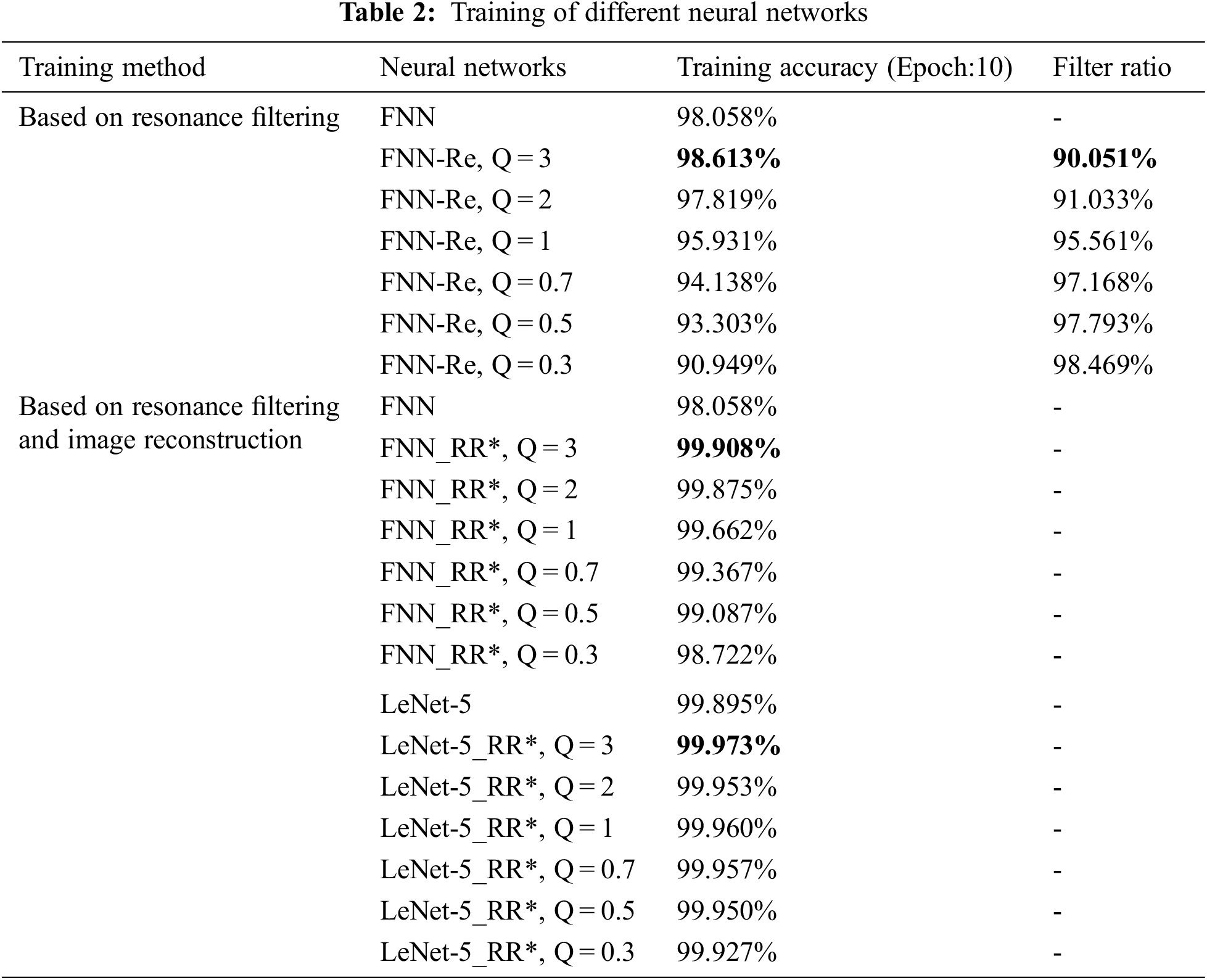
At the end of this section, all the experimental neural networks are accurately summarized in Tab. 2 for observation and comparison. It should be noted that the data set used in the experiment is the MNIST database. All research and discussion are carried out on this basis.

6  Conclusion

In this paper, on the basis of extracting individual features of image skeleton and image edge, a mixed feature extraction method of resonance layer is designed before neural network to reconstruct training images. The feature extraction efficiency of neural network can be improved by efficient expression of common features and individual features of training set images. This heuristic modification improves the feature extraction efficiency of neural network. The future work can try to transplant the resonance layer to more kinds of neural network structures. You can also use different data sets other than MNIST for validation; More importantly, the algorithm can be optimized to improve the efficiency of parallel computing in the future.

Funding Statement: This paper is supported by National Natural Science Foundation of China (Youth program, No. 82004499, Youwei Ding, https://www.nsfc.gov.cn/), Project of Natural Science Research of the Universities of Jiangsu Province (No. 20KJB520030, Yihua Song, http://jyt.jiangsu.gov.cn/) and the Qing Lan Project of Jiangsu Province (Xia Zhang, http://jyt.jiangsu.gov.cn/).

Conflicts of Interest: The authors declare that they have no conflicts of interest to report regarding the present study.

References

 1.  M. Wan, X. Chen, T. Zhan, C. Xu, G. Yang et al., “Sparse fuzzy two-dimensional discriminant local preserving projection (SF2DDLPP) for robust image feature extraction,” Information Sciences, vol. 563, pp. 1–15, 2021. [Google Scholar]

 2.  W. Li, Q. Huang and G. Srivastava, “Contour feature extraction of medical image based on multi-threshold optimization,” Mobile Networks and Applications, vol. 26, pp. 381–389, 2021. [Google Scholar]

 3.  R. Sharma, A. Singh, A. Kavita, N. Jhanjhi, M. Masud et al., “Plant disease diagnosis and image classification using deep learning,” Computers, Materials & Continua, vol. 71, no. 2, pp. 2125–2140, 2022. [Google Scholar]

 4.  W. Hao, Q. Liu and X. Liu. “A review on deep learning approaches to image classification and object segmentation,” Tech Science Press, vol. 1, no. 1, pp. 1–5, 2018. [Google Scholar]

 5.  Q. Huang, Y. Zhou, L. Tao, W. Yu, Y. Zhang et al., “A Chan-vese model based on the markov chain for unsupervised medical image segmentation,” Tsinghua Science and Technology, vol. 26, no. 6, pp. 833–844, 2021. [Google Scholar]

 6.  C. Wu and Z. Cao, “Entropy-like distance driven fuzzy clustering with local information constraints for image segmentation,” The Journal of China Universities of Posts and Telecommunications, vol. 28, no. 1, pp. 24–40, 2021. [Google Scholar]

 7.  M. Ganesh, M. Naresh and C. Arvind, “MRI brain image segmentation using enhanced adaptive fuzzy K-means algorithm,” Intelligent Automation & Soft Computing, vol. 23, no. 2, pp. 325–330, 2017. [Google Scholar]

 8.  T. Malisiewicz, A. Gupta and A. A. Efros. “Ensemble of exemplar-SVMs for object detection and beyond,” in Proc. of the 2011 Int. Conf. on Computer Vision, Barcelona, Spain, pp. 89–96, 2021. [Google Scholar]

 9.  D. Zhang, J. Hu, F. Li, X. Ding, A. K. Sangaiah et al., “Small object detection via precise region-based fully convolutional networks,” Computers, Materials & Continua, vol. 69, no. 2, pp. 1503–1517, 2021. [Google Scholar]

10. C. Song, X. Cheng, Y. Gu, B. Chen and Z. Fu, “A review of object detectors in deep learning,” Journal on Artificial Intelligence, vol. 2, no. 2, pp. 59–77, 2020. [Google Scholar]

11. M. Ju, J. Luo, Z. Wang and H. Luo, “Adaptive feature fusion with attention mechanism for multi-scale target detection,” Neural Computing and Applications, vol. 33, pp. 2769–2781, 2021. [Google Scholar]

12. P. Han, M. Zhang, J. Shi, J. Yang and X. Li, “Chinese Q&A community medical entity recognition with character-level features and self-attention mechanism,” Intelligent Automation & Soft Computing, vol. 29, no. 1, pp. 55–72, 2021. [Google Scholar]

13. G. Hou, J. Qin, X. Xiang, Y. Tan and N. Xiong, “Af-net: A medical image segmentation network based on attention mechanism and feature fusion,” Computers, Materials & Continua, vol. 69, no. 2, pp. 1877–1891, 2021. [Google Scholar]

14. Y. Chen, L. Liu, V. Phonevilay, K. Gu, R. Xia et al., “Image super-resolution reconstruction based on feature map attention mechanism,” Applied Intelligence, vol. 51, pp. 4367–4380, 2021. [Google Scholar]

15. S. Zhang, J. Yang and B. Schiele, “Occluded pedestrian detection through guided attention in CNNs,” in Proc. of the IEEE Conf. on Computer Vision and Pattern Recognition, Salt Lake City, UT, USA, pp. 6995–7003, 2018. [Google Scholar]

16. X. Xu, T. Gao, Y. Wang and X. Xuan, “Event temporal relation extraction with attention mechanism and graph neural network,” Tsinghua Science and Technology, vol. 27, no. 1, pp. 79–90, 2021. [Google Scholar]

17. K. Saeed, M. Tabedzki, M. Rybnik and M. Adamski, “K3M: A universal algorithm for image skeletonization and a review of thinning techniques,” Applied Mathematics and Computer Science, vol. 20, no. 2, pp. 317–335, 2010. [Google Scholar]

18. J. Canny, “A computational approach to edge detection,” IEEE Transactions on Pattern Analysis and Machine Intelligence, vol. PAMI-8, no. 6, pp. 679–698, 1986. [Google Scholar]

19. Z. Su, W. Liu, Z. Yu, D. Hu, Q. Liao et al., “Pixel difference networks for efficient edge detection,” in Proc. of the IEEE/CVF Int. Conf. on Computer Vision (ICCV), Montreal, QC, Canada, pp. 5117–5127, 2021. [Google Scholar]

20. J. He, S. Zhang, M. Yang, Y. Shan and T. Huang, “Bi-DirectionalCascade network for perceptual edge detection,” in Proc. of the IEEE/CVF Conf. on Computer Vision and Pattern Recognition (CVPR), Long Beach, CA, USA, pp. 3828–3837, 2019. [Google Scholar]

21. B. Wang, L. Chen and Z. Zhang, “A novel method on the edge detection of infrared image,” Optik, vol. 180, pp. 610–614, 2019. [Google Scholar]

22. Y. Liu, M. Cheng, D. Fan, L. Zhang, J. Bian et al., “Semantic edge detection with diverse deep supervision,” International Journal of Computer Vision, vol. 130, pp. 179–198, 2022. [Google Scholar]

23. Y. LeCun, L. Bottou, Y. Bengio and P. Haffner, “Gradient-based learning applied to document recognition,” Proceedings of the IEEE, vol. 86, no. 11, pp. 2278–2324, 1998. [Google Scholar]

24. J. Schmidhuber. “Deep learning in neural networks: An overview,” Neural Networks, vol. 61, pp. 85–117, 2015. [Google Scholar]

25. M. A. Nielsen, “The four fundamental equations behind back propagation,” in The Neural Networks and Deep Learning, San Francisco, CA: Determination press, vol. 25, pp. 9–12, 2015. [Google Scholar]

26. X. Zhang, X. Wang and C. Gu, “Online multi-object tracking with pedestrian re-identification and occlusion processing,” The Visual Computer, vol. 37, pp. 1089–1099, 2021. [Google Scholar]

27. Y. Tian, P. Luo, X. Wang and X. Tang, “Deep learning strong parts for pedestrian detection,” in Proc. of the IEEE Int. Conf. on Computer Vision, Santiago, Chile, pp. 1904–1912, 2015. [Google Scholar]

28. W. Ouyang, H. Zhou, H. Li, Q. Li, J. Yan et al., “Jointly learning deep features, deformable parts, occlusion and classification for pedestrian detection,” IEEE Transactions on Pattern Analysis and Machine Intelligence, vol. 40, no.8, pp. 1874–1887, 2017. [Google Scholar]