LSTM Based Spectrum Prediction for Real-Time Spectrum Access for IoT Applications

1  Introduction

Demand for spectrum is expected to increase drastically in the next-generation wireless network, which is expected to support extremely high data rates and more numbers of connected devices. Conventional static spectrum allocation policies can no longer provide substantial improvement due to the inefficient use of the wireless spectrum [1]. Federal Communication Commission (FCC) reported [2] that majority of the spectrum allocated to licensed users remains underutilized at any given time and location. To solve the contradiction between spectrum scarcity and spectrum under-utilization cognitive radio network (CRN), which allows unlicensed user/secondary users to opportunistically access the spectrum in such a way that it does not cause any harmful interference to the licensed user/primary user [3,4] evolved. The first step towards realizing Cognitive Radio (CR) requires the Secondary User (SU) to sense the radio spectrum state (RSS), which consumes a considerable amount of time and energy. This can be eliminated with the introduction of spectrum prediction, which forecasts future channel states based on historical information [5]. Spectrum prediction finds many potential applications in future wireless networks such as Cooperative Relay Network (CRN), smart grid, 5G network, and IoT devices. Spectrum prediction techniques based on different methods like Linear prediction Auto-Regressive (AR), Moving Average(MA), Auto-Regressive Moving Average(ARMA), Autoregressive Integrated Moving Average (ARIMA) models [6–8], Markov models based models [9–12] have been carried out. However, the majority of the existing work is based on conventional statistical techniques or shallow models to predict the spectrum state. Deep Learning (DL), a branch of machine learning inspired by the human brain, fuelled by more available computing power, has shown excellent performance in image classification, target recognition [13], natural language processing [14]. However, in DL, not all architecture is suitable for all applications.

Recurrent neural network (RNN) is one such architecture suitable for time series data, which is, in this case, for spectrum prediction. RNN suffers from vanishing and exploding gradients. Therefore, Long Short Term Memory (LSTM), an improved version of RNN, was introduced to overcome the above-said disadvantage. LSTM has been employed in [15,16], to predict the spectrum state. The primary objective of spectrum prediction is to enhance the throughput of SUs. Authors in [5] propose a redesigned frame structure that incorporates spectrum prediction, such that they select only those channels for prediction, which are predicted to be free. In [17], spectrum prediction and channel selection strategy based on online learning techniques are proposed. Authors in [18] propose a prediction and sensing-based spectrum sharing model where cooperative spectrum prediction is employed. However, it uses a conventional statistical method for signal and its arrival. It employs Multi-layer perceptron (MLP), which is unsuitable for historical dependencies and ineffective for time series data. In [19], authors use LSTM for prediction-based spectrum access, optimal sensing interval, which is used as output length of LSTM for each channel is computed for each channel individually makes implementation complex in real-time due to random nature of radio spectrum. Authors in [20] proposed a hybrid approach combining Bayesian and Exponential Weighted Moving Average (EWMA) approaches for spectrum hole prediction, which is based on the classical approach. In [21], the authors conduct a detailed survey of spectrum prediction in a cognitive radio network. There are few software-defined radio-based works for spectrum sharing [22–25]. CNN architecture has been used recently to solve object detection, identification and classifications [26,27]. But LSTM is used to solve the time series problem, which is utilized in this work. There are few spectrum prediction works [28,29]. A deep neural network called Residual network and Channel and Spatial attention modules (RCS) with Gated Recurrent Unit network(RCS-GRU) is presented [28] for detecting occupancy correlation of different frequency channels by the PU. It also predicts the spectrum occupancy of the future next time slot. A Hybrid Spectrum Access with Spectrum Prediction and Cooperation (HSA-SPC) is proposed [29] with spectrum prediction to improve the throughput of Cognitive users. The multiuser environment is considered and closed-form expression for the throughputs derived. But there is no substantial work on using spectrum prediction results to allow access to the spectrum based on real-world data.

Contribution: We develop a framework, namely Positive Prediction and Sensing Based Spectrum Access (PPSBSA), by employing Encoder-Decoder LSTM to predict for two-time slots simultaneously and use the prediction result to help Secondary User (SU) achieve lower waiting time and hence higher capacity.

The remainder of this paper is organized as follows: In Section 2, the system model describes the model as a physical entity that discusses the construction of the data set, the frame structure for secondary users. Section 3 consists of the proposed Positive Prediction and sensing-based spectrum access (PPSBSA) framework. Section 4 discusses LSTM in a quite elaborate manner. Section 5 lists the parameters used in the evaluation. Finally, Section 6 has experimental results in the form of graphs and tables, followed by a conclusion in Section 7.

2  System Model

The architecture consists of a Secondary user transmitter node (SU-T), which acts as a device in a cognitive radio network (CRN) based cellular network where devices work as the secondary user (SU). In contrast, cellular-based users are the primary user (PU). SU-T can convey information with multiple devices (SU-R1, SU-R2, SU-R3, and SU-R4). Two support nodes, transmit node one and send node two, are assigned to SU-T to help in the transmission of SU-T. In this work, the prediction of the spectrum state is carried out for two-time slots; therefore, each node TN-1 and TN-2 will transmit information to two receiver nodes. For example, TN-1 will transmit to SU-R1 and SU-R2, whereas TN-2 will transmit to SU-R3 and SU-R4.

It is assumed that SU-T distributes information to both nodes before its transmission to receiver nodes via some wired network. Both the nodes are allocated N numbers of spectrum points, which are distinct to avoid interference. Both nodes transmit in a parallel fashion such that at (t + 1),the slot TN-1 transmit to SU-R1, TN-2 transmits to SU-R3, while at (t + 2),the slot TN-1 transmits to SU-R2 and TN-2 transmits to SU-R4. Receiver nodes are aware of the spectrum points allocated to nodes through some information exchange.

Spectrum prediction is to predict the spectrum state in the next slot by mining the internal relationship of historical spectrum data. That is given spectrum measurement data (in terms of PSD) for current time slot t and previous time slots, Xt-4, Xt-3, Xt-2, Xt-1, Xt is fed as input to Encoder-Decoder LSTM network which has been trained to discover the internal relationship. Then the output of Encoder-Decoder LSTM is the prediction of PSD values for t + 1 and t + 2 slots. The Fig below shows dataset construction for a single spectrum point.

From Fig. 2, for each spectrum point, both nodes are trained on 100 s of such input sequences (Ii) and corresponding label (Oi), where i = 1, 2, 3,…K, where K is a total number of sequences that are fed to Encoder-Decoder LSTM to train and discover internal relationship so that the network predicts the spectrum state for next two slots when fed with any unseen sequence Iu where u ∉ K. Data set for each spectrum point for which prediction is carried out is shuffled in advance and thereby divided into training set and test placed to avoid sample distribution imbalance. Similarly, both nodes are trained for all distinct N spectrum points allocated to them.

As shown in Fig. 1, the nodes have a single antenna such that it first predicts allocated spectrum points then senses only that spectrum point, which is predicted to be free (Positive), not for busy/occupied (Negative). At (t + 1),the slot data is transmitted by TN-1 and TN-2 to SU-R1 and SU-R3, respectively. For a particular scenario, let the status of spectrum points as predicted and sensed during 1st slot be given by Tab. 1.

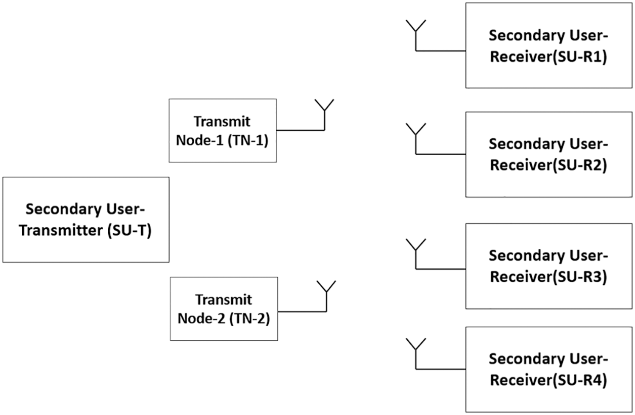
Figure 1: Architecture of proposed framework

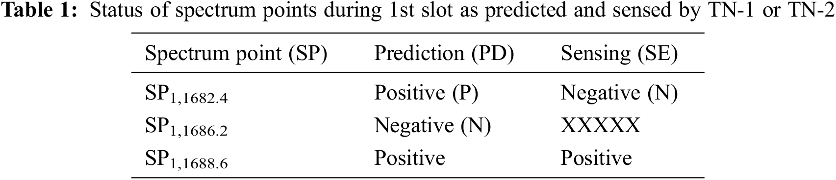
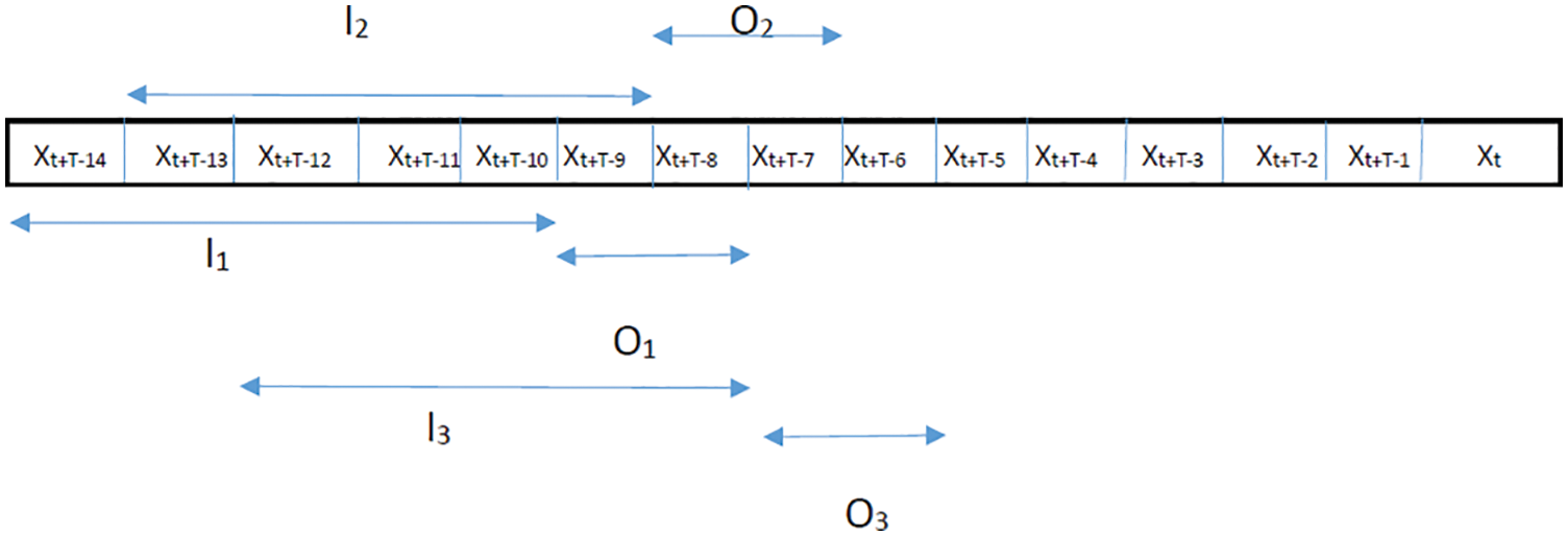
Figure 2: Dataset construction for single spectrum point

Frame structure corresponding to Tab. 1 is given as shown below

In Tab. 1, SP 1.1682.4 denotes 1st time slot 1682.4 MHz spectral point. In general, SP i,k denotes ith time slot on k MHz spectrum point. Fig. 3 Shows the frame structure of transmission for the scenario given in Tab. 1, where two transmission slots are not utilized for data transmissions because, as for Tab. 1, prediction and sensing do not give positive results. But the third spectral point in Tab. 1 provides both sensing and prediction positive results. So that is utilized for data transmission.

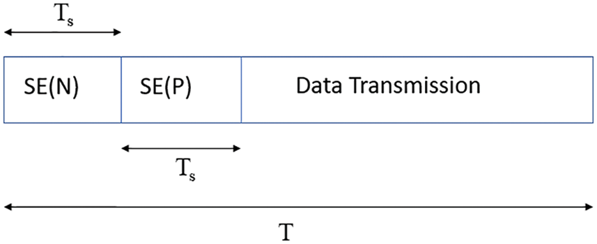
Figure 3: Frame structure for the scenario given the Tab. 1

From Tab. 1, we can observe that sensing is carried out for 1682.4 SP as the prediction is Positive. However, sensing is Negative; therefore, it moves ahead and senses 1688.6 MHz SP. Since the forecast for 1686.2 MHz is negative, both prediction and sensing for 1688.6 MHz SP are Positive. Nodes perform prediction of SPs in chronological order as allocated to them; sensing is only shown if the forecast is Positive for the same. Nodes use the energy detection method to sense the spectrum where PSD is compared with the threshold to decide whether PU is present. In Tab. 1, only the status of some spectrum points is shown for the representation purpose of the PPSBT framework and is not the actual number of spectrum points allocated to nodes.

Similarly, at (t + 2),the slot data is transmitted by TN-1 and TN-2 to SU-R2 and SU-R4, respectively. Considering a particular scenario, let the status of spectrum points as given by the PPSBSA framework during 2nd slot be provided, as shown below.

Frame structure corresponding to Tab. 2 is given by, as shown below:

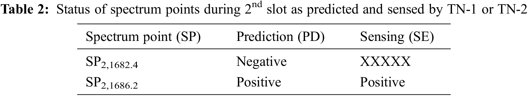
From Tab. 2, 1686.2 MHz spectral points provide a positive result for prediction as well as sensing, so immediately, the spectral point of the second frequency is used for data transmission, as shown in the frame structure in Fig. 4.

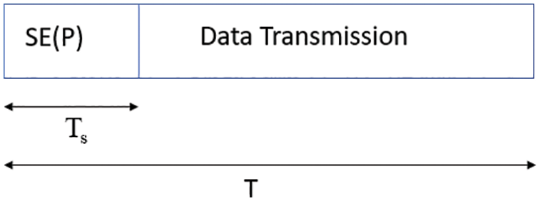
Figure 4: The frame structure for the Tab. 2 scenario

Here since the prediction for 1682.4 MHz, SP is negative; hence directly, 1686.2 MHz SP is sensed and found to be positive.

3  Positive Prediction and Sensing Based Spectrum Access (PPSBSA) Framework

Framework, as described above in Fig. 5, uses spectrum prediction results for transmission. For simulation, spectrum prediction is performed on a testing sequence (I) that is not part of the training set. The input sequence (l) and the corresponding label (O) used for the prediction can be visualized as a real-time sequence. When fed to the LSTM network trained with the training set, the testing sequence I produce a forecast for two slots ahead O’. In real-time, spectrum sensing is performed to determine whether the prediction is correct or not; however, in simulation, we compare O’ with O to determine whether the prediction was accurate, where O is regarded as a sensed value.

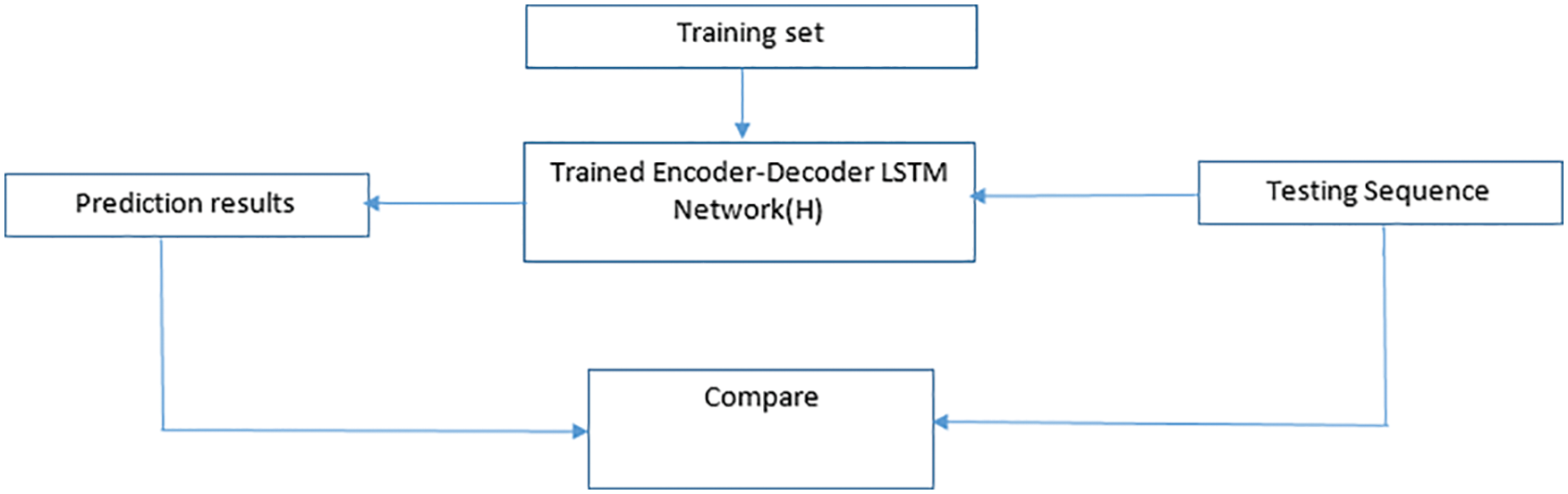
Figure 5: Positive prediction and sensing-based spectrum sharing framework flow chart

The above model consists of 3 steps; during step-1 the training set [Ii->Oi] is fed to train the Encoder-Decoder LSTM network so that model is built

H=T[Ii→Oi],i=1,2,3,…K. (1)

Here T designates the training of the LSTM network with a total K sequence, and H is the Encoder-Decoder LSTM network, which has been trained to discover internal relationships and predict the spectrum state for the next two slots. During step-2 the testing sequence I is fed to the trained Encoder-Decoder LSTM network designated by H, which results in prediction values for two slots ahead given by

Ot′=H[I],t=1,2. (2)

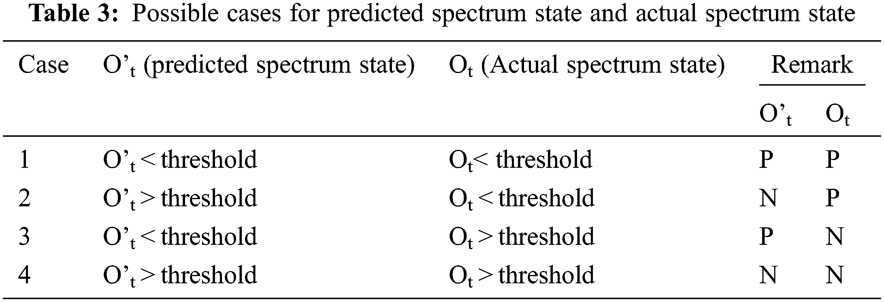
Finally, in step-3, the label corresponding to the testing sequence (I), It is compared with the prediction result Ot’. Moreover, t = 1, 2, is used to represent spectrum prediction for 1st and 2nd slot. Based on the above, there can be four cases.

Tab. 3 shows the possible outcome after the LSTM network outcome in comparison with the actual spectrum state Qt. If the predicted outcome O, t and actual outcome Qt is less than the threshold, the net outcome is declared as positive “P”. If any of the outcomes is greater than the threshold the corresponding net outcome is declared as negative “N”.

4  LSTM Network for Spectrum Prediction

A recurrent neural network (RNN) is validated to solve time series problems. However, they fail to handle ‘long term dependencies,’ this problem was explored in detail by Hochreiter (1991) and Bengio et al. (1994). In 1997, Hochreiter & Schmidhuber introduced long short term memory (LSTM), a special kind of RNN which are capable of learning long term dependencies. The key to LSTM is the cell state with information being added or removed from the cell state through three gates, namely the input gate, forget gate, and output gate.

The first gate that we refer to is forgotten; it decides what information will be discarded from the cell state. The sigmoid layer determines by outputting a number between 0 and 1. 1 means to retain the information entirely and 0 means to get off the information.

ft=σ(Wxf.xt+Wsf.st−1+bf) (3)

The input gate which decides whether which values to update, using sigmoid layer.

it=σ(Wxt.xt+Wst.st−1+bt) (4)

Additionally, tanh layer creates a vector of new candidate values, which is combined with the input gate to update the cell state and thereby cell state is given by,

ct′=tanh(Wxc.xt+Wsc.st−1+bc) (5)

ct=it∗ct′+ft∗ct−1 (6)

Moreover, the output gate and hidden state are given as,

ot=σ(Wxo.xt+Wso.st−1+bo) (7)

st=ot∗tanh⁡(ct) (8)

4.1 LSTM Encoder-Decoder Architecture

In this work, encoder-decoder, LSTM, is used since the forecasting of spectrum state is carried out for two-time steps into the future. Encoder-Decoder LSTM as shown in Fig. 7 was developed for natural language processing, particularly in areas of text translation, where it has proven to be excellent.

The Encoder layer consists of LSTM memory cells (as shown in Fig. 6) which takes PSD values as input; the cell state and hidden state of the last memory cell (M is the total LSTM memory cells) in the encoder are fed as the initial cell state and hidden state respectively to the first memory cell in the decoder LSTM network. Each LSTM memory cell produces an output that is fed as input to the next LSTM sequentially since the regression-based prediction is used; hence dense layer is used in the output layer.

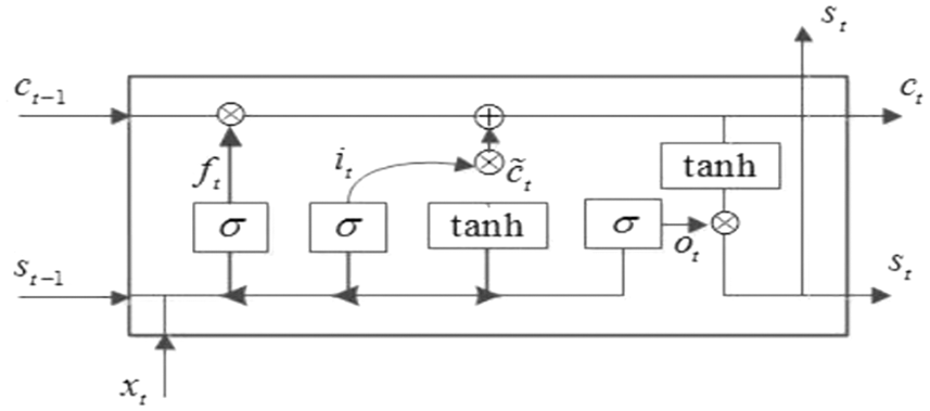
Figure 6: Structure of an LSTM cell memory

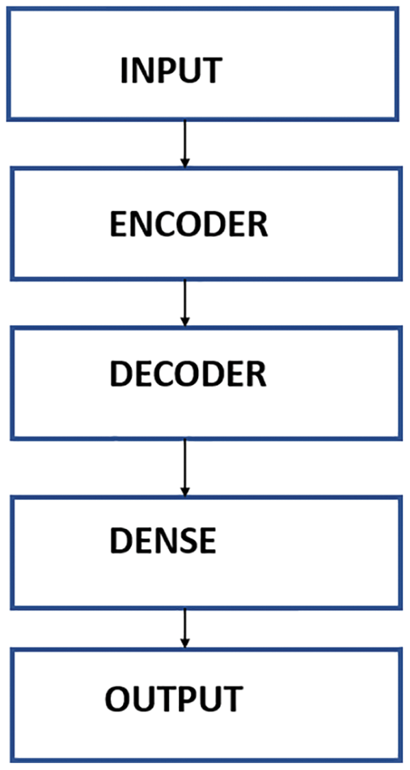
Figure 7: Encoder-Decoder LSTM architecture

5  Evaluation Metrics

Here in this section, different metrics/parameters related to the experimental evaluation are discussed.

5.1 Waiting Time

Waiting time (WT) is defined as the time elapsed between the beginning of the timeslot and actual data transmission. Mathematically waiting time for 1st timeslot is given as follows:

WT(1)=Tp+∑i=1N⁡Ts,i[SP1,i=P] (9)

For second slot WT is given by

WT(1)=Tp+∑i=1N⁡Ts,i[SP2,i=P] (10)

Eqs. (9) and (10) are identical except single literal, which make waiting time for either 1st or 2nd-time slot. Here i is the specific spectrum point in chronological order as allocated to nodes. For example, from Tab. 1, for 1682.4 MHz, i is 1, and for 1686.2 MHz, i is two and so on. TP is the time required to predict the status of N spectrum points in a parallel manner. Ts,i Is sensing time of the ith spectrum point and is equal to Ts when the prediction is positive (condition inside square bracket) else it’s 0. Waiting time depends on the real-time availability of the radio spectrum. That is only if both prediction and sensing are positive only then the user can access the given time slot; however, if the forecast is favorable and sensing is negative, it will lead to increased waiting time and reduced C and hence termed a false prediction (FP).

If FP = j, it means j number of times (j < N) the prediction was found to be positive while sensing was negative, and node access the spectrum by (j + 1)the time. Based on this, the generic formulae for waiting time is given as:

WT=Tp+Ts(j+1) (11)

From Eq. (11), it is evident that the time wasted for unnecessarily spectrum sensing is,

W=Tsj (12)

5.2 Classification Accuracy

To evaluate the classification accuracy, the PSD values are converted into binary values. This conversion takes place according to threshold levels if PSD values are greater than threshold values, then the corresponding PSD value is set as 1 (indicating the presence of the primary user) else 0.

CA=1N∑t=1N⁡(Bt) (13)

where Bt = 1, when the predicted channel state and real channel state are the same (occupied or idle), else it is 0.

5.3 Capacity

Combining Eqs. (9), (10). Capacity is given as

CAPACITY(C)=(T−WT)Tlog2(1+SNR) (14)

Signal-to-Noise Ratio(SNR) is used to calculate the capacity.

6  Experimental Setup and Performance Analysis

Spectrum data from the RWTH Aachen University spectrum data measurement campaign [22] is used. Correctly, the band 1876–1886 MHz is used. The 10 MHz bands are intentionally selected since it consists of spectrum points with different and unique occupational status to emulate real-world scenarios.

The resolution bandwidth is set to 200 KHz. 3-fold cross-validation for the 1st and 2nd-time slot for each spectrum point is computed. The mean accuracy for the 1st and 2nd slot is shown in Fig. 8 and Fig. 9 respectively.

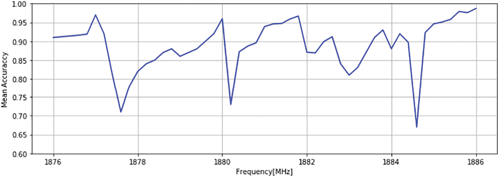
Figure 8: Mean accuracy for (t + 1) th slot

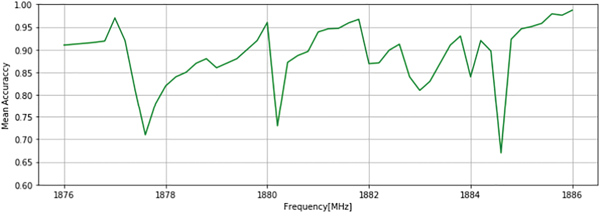
Figure 9: Mean accuracy for (t + 2) th slot

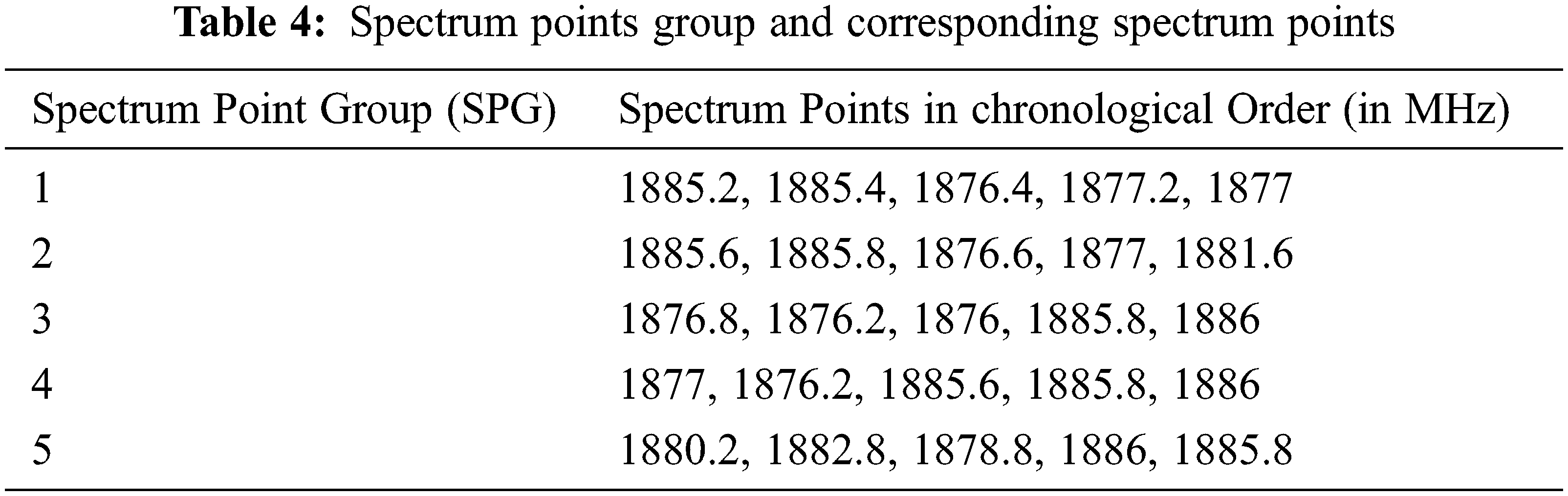
The entire spectrums are grouped into five groups. In each group, 5 spectral points are considered. Any transmitting node will be allocated one spectrum point group on which the node may employ sensing and prediction for data transmission.

It is quite evident that in both cases, the mean accuracy of each SP is quite similar. The mean of ‘mean accuracy’ for 1st and 2nd-time slots are 0.9177 and 0.9167, respectively. Each node (TN-1 and TN-2) is allocated a particular Spectrum Point Group (SPG), which consists of 5 spectrum points. In Tab. 4, in each group, five spectrum points are shown in proper chronological order in terms of the order in which nodes access them.

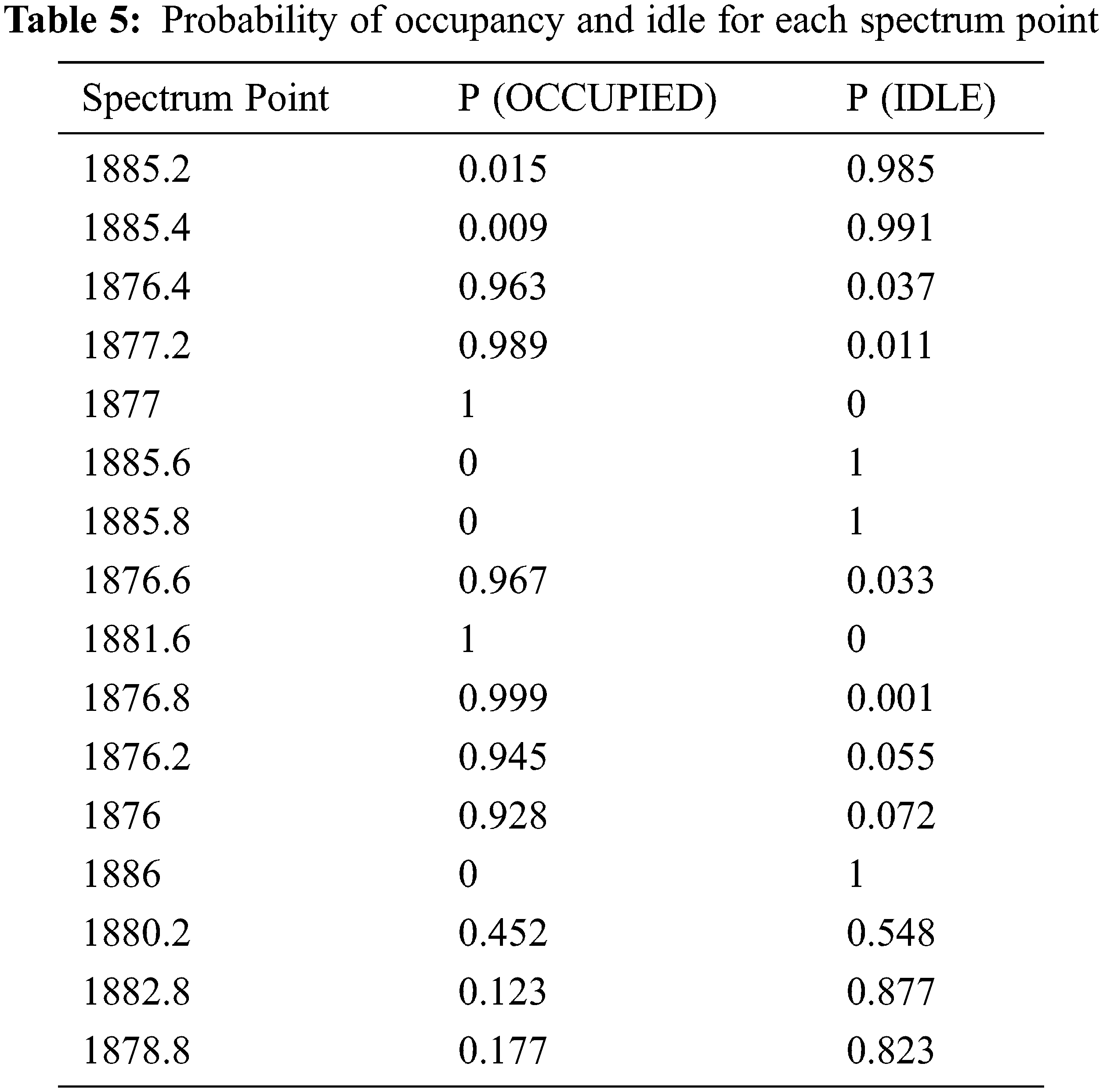
As explained earlier, spectrum points with different occupational patterns are considered to study their impact on waiting time. In the radio spectrum, the status of occupancy of spectrum points at a given time in any band is dynamic. However, the occupancy does depend on the historical occupational status to a large extent. Therefore, the probability statistics of each spectrum point are essential to be computed.

Using Tab. 5 for each spectral point, the probability of occupancy and ideal can be interpreted. Using those probabilities, the transmitting node may check the spectral point for use, which selects the spectrum which has the highest probability of idle and lowest probability of occupancy. This probability-based checking reduces the time for the selection of transmission frequency and improves performance.

Each node is assigned a group of five spectrum points, which are selected such that it emulates the possible scenarios in the real world, SNR at SU is considered to be 20 dB.

Based on the groups mentioned above, an experiment was conducted for each group individually. The time required to predict five spectrum points is 3.7 msec (Tp), while the time needed to sense each time slot is given as 2.6 msec (Ts) [5]. Waiting for time and capacity for each time slot are computed from Eqs. (9), (10) and (14). The proposed PPSBSA framework from here on will be referred to as the Proposed framework (PF).

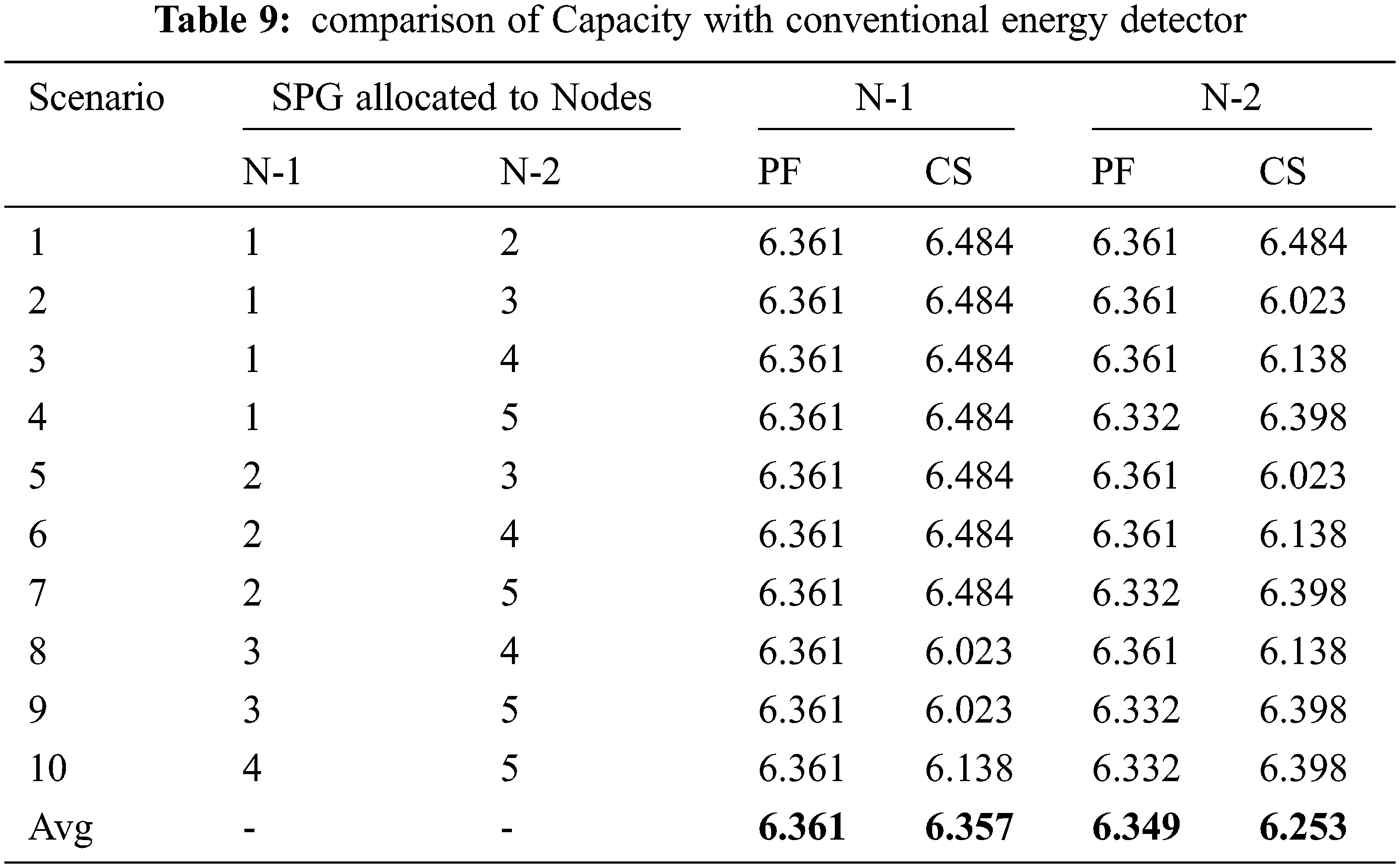
Tabs. 6, 7 provides computation of waiting time and throughput for the first and second-time slot, respectively. The waiting time and average capacity for the proposed method are compared with the conventional energy detector sensing method of energy detector.

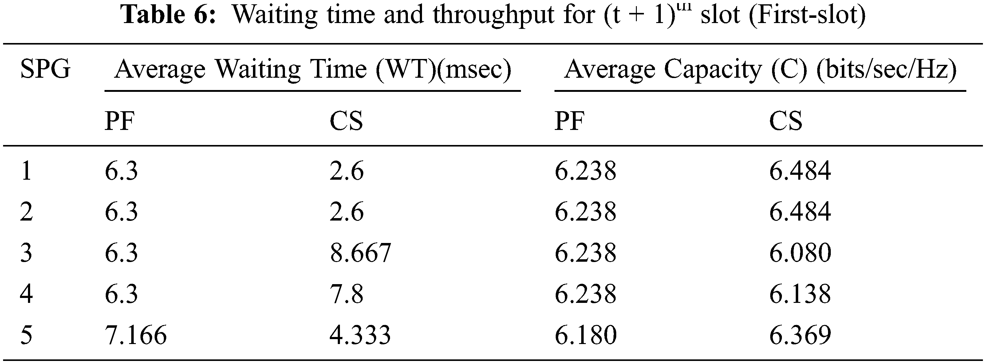
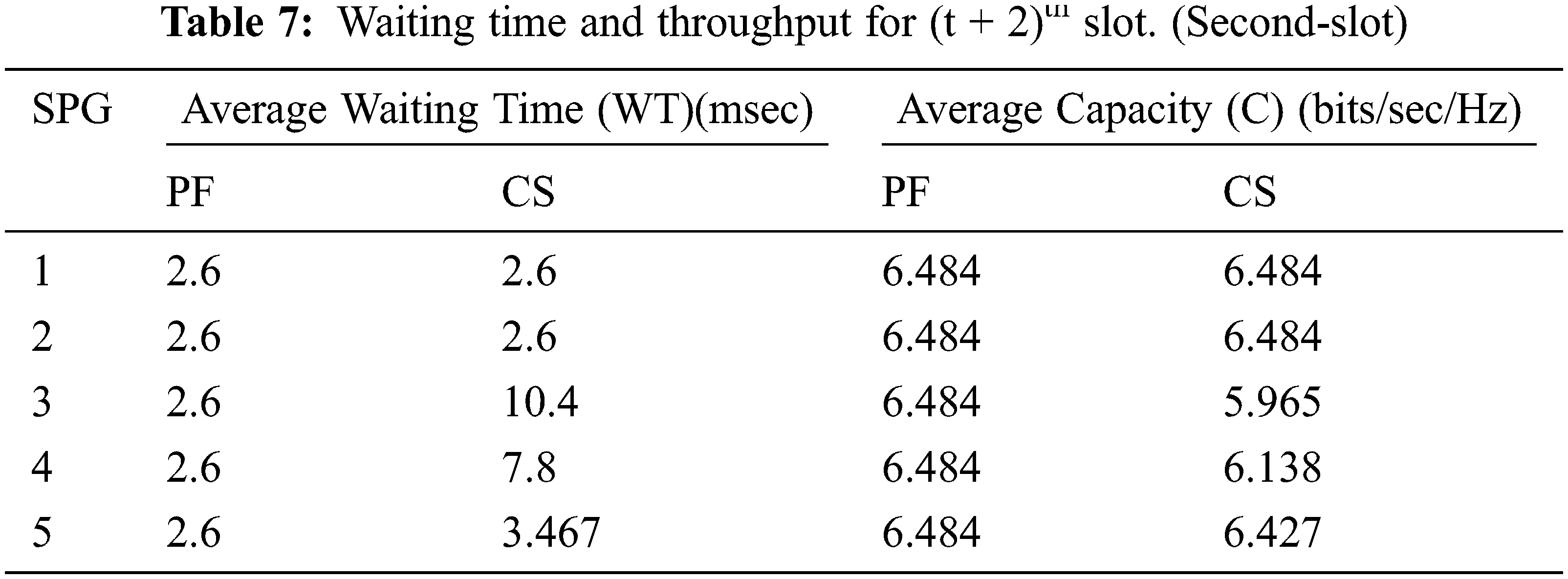
From Tabs. 6 and 7, it is evident the average waiting time and capacity achieved by the proposed system is almost the same as the conventional energy detector sensing method, which proves that even though the proposed system is complex, it takes only the same complexity low complex algorithm of energy detector.

CS stands for conventional sensing, which is the energy-based detector. To emulate real-time scenarios as discussed earlier, both the nodes are allocated a particular spectrum point group. Therefore, we consider the combination of all the groups assigned to both nodes.

6.1 Comparison of Performance

The proposed method performance is compared with conventional low complex energy detectors. The waiting time and the capacity achieved performance metrics are used.

In Tab. 8 N-1, N-2 represents transmission nodes 1 & 2 and the waiting time of nodes 1 & 2 for the proposed scheme and the conventional scheme is recorded under N-1 and N-2 columns.

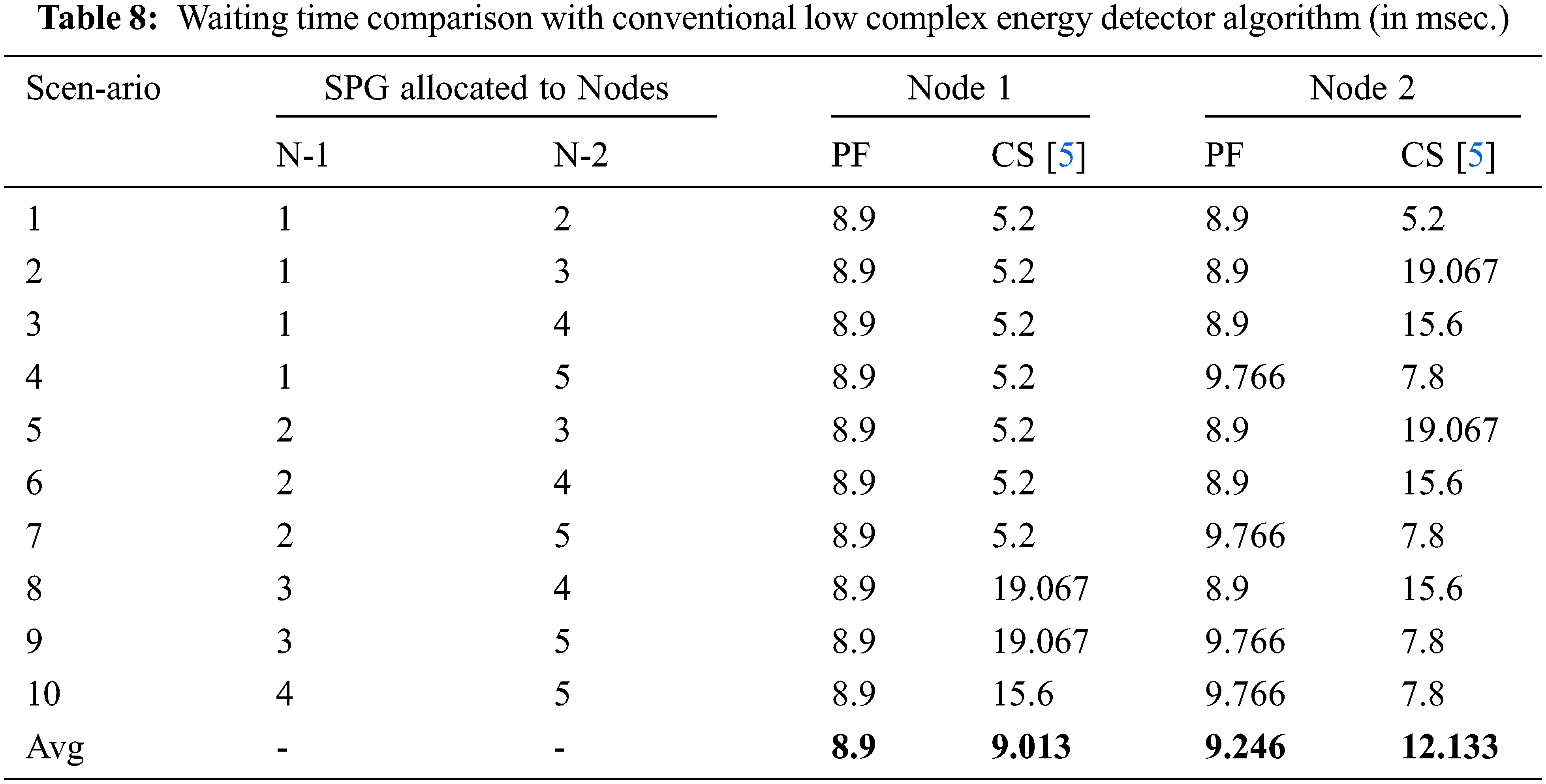
From the above Tab. 8, it is very evident that the proposed PPSBSA has a waiting time lower energy detection based on Conventional Sensing. Authors in [5] considered energy detection-based spectrum sensing since it is efficient and faster than many spectrum sensing and therefore been considered to compare with the proposed framework. On average, the waiting time is lesser for the PPSBSA framework by 0.1134 msec for 1st slot and by 2.887 msec for 2nd slot.

Specifically, when nodes are allocated those spectrum points which have a higher probability of being occupied, the proposed PPSBSA framework is quite better when to compared with conventional sensing, as evident from Tabs 6 and 7 (Looking at spectrum point groups of 4 and 5). Therefore, this framework will be beneficial for D2D, M2 M communication, wherein devices and machines are part of a secondary network that uses the spectrum of the primary user network (cellular network) where more spectrum is occupied for the most amount of time. Based on Tab. 8, the achievable capacity was calculated.

7  Conclusion

Owing to new diverse applications (like M2 M, V2Vcommunications) in next-generation wireless networks, the availability of spectrum is slated to be scary since a large part of the available spectrum will be reserved for the cellular network-based user (primary user). This work proposes Positive Prediction and Sensing Based Spectrum Access (PPSBSA) to predict the Radio Spectrum State (RSS) for two-time slots, thereby reducing the time required for sensing the spectrum. Results show nodes employing the proposed framework achieve lesser waiting time, especially when the spectrum point has a higher chance of being occupied, the margin is even higher. Therefore, this proposed framework is suitable for next-generation wireless networks wherein diverse IoT applications can satisfy their need for spectrum. In future research can be carried out on training LSTM, correlation of specific time, and occupancy.

Funding Statement: The authors received no specific funding for this study.

Conflicts of Interest: The authors declare that they have no conflicts of interest to report regarding the present study.

References

 1.  S. Haykin, “Cognitive radio: Brain-empowered wireless communications,” IEEE Journal on Selected Areas in Communications, vol. 23, no. 2, pp. 201–220, 2015. [Google Scholar]

 2.  S. Force, “Spectrum policy task force report,” Federal Communications Commission ET Docket, vol. 135, pp. 1–73, 2002. [Google Scholar]

 3.  J. Mitola Iii, “Cognitive radio for flexible mobile multimedia communications,” Mobile Networks and Applications, vol. 6, no. 5, pp. 435–441, 2001. [Google Scholar]

 4.  Q. Wu, G. Ding, J. Wang and Y. D. Yao, “Spatial-temporal opportunity detection for spectrum-heterogeneous cognitive radio networks Two-dimensional sensing,” IEEE Transactions on Wireless Communications, vol. 12, no. 2, pp. 516–526, 2013. [Google Scholar]

 5.  J. Yang and H. Zhao, “Enhanced throughput of cognitive radio networks by imperfect spectrum prediction,” IEEE Communications Letters, vol. 19, no. 10, pp. 1738–1741, 2015. [Google Scholar]

 6.  Z. Wen, T. Luo, W. Xiang, S. Majhi and Y. Ma, “Autoregressive spectrum hole prediction model for cognitive radio systems,” in ICC Workshops-2008 IEEE Int. Conf. on Communications Workshops, Beijing, pp. 154–157, 2008. [Google Scholar]

 7.  S. Yarkan and H. Arslan, “Binary time series approach to spectrum prediction for cognitive radio,” in IEEE 66th Vehicular Technology Conf., Baltimore, MD, USA, pp. 1563–1567, 2007. [Google Scholar]

 8.  A. A. Tabassam, M. U. Suleman, S. Khan and S. H. R. Tirmazi, “Spectrum estimation and spectrum hole opportunities prediction for cognitive radios using higher-order statistics,” in IEEE Int. Conf. on Wireless Advanced, London, UK, pp. 213–217, 2011. [Google Scholar]

 9.  Z. Chen, N. Guo, Z. Hu and R. C. Qiu, “Experimental validation of channel state prediction considering delays in practical cognitive radio,” IEEE Transactions on Vehicular Technology, vol. 60, no. 4, pp. 1314–1325, 2011. [Google Scholar]

10. V. K. Tumuluru, P. Wang and D. Niyato, “Channel status prediction for cognitive radio networks,” Wireless Communications and Mobile Computing, vol. 12, no. 10, pp. 862–874, 2012. [Google Scholar]

11. I. A. Akbar and W. H. Tranter, “Dynamic spectrum allocation in cognitive radio using hidden markov models: Poisson distributed case,” in IEEE Int. Conf. on SoutheastCon, Richmond, VA, USA, pp. 196–201, 2007. [Google Scholar]

12. E. Chatziantoniou, B. Allen and V. Velisavljević, “An HMM-based spectrum occupancy predictor for energy efficient cognitive radio,” in Annual Int. Symposium on Personal, Indoor, and Mobile Radio Communications (PIMRC), London, UK, pp. 601–605, 2013. [Google Scholar]

13. L. Wang, T. Liu, G. Wang, K. L. Chan and Q. Yang, “Video tracking using learned hierarchical features,” IEEE Transactions on Image Processing, vol. 24, no. 4, pp. 1424–1435, 2015. [Google Scholar]

14. Y. Xiang, Q. Chen, X. Wang and Y. Qin, “Answer selection in community question answering via attentive neural networks,” IEEE Signal Processing Letters, vol. 24, no. 4, pp. 505–509, 2017. [Google Scholar]

15. L. Yu, J. Chen and G. Ding, “Spectrum prediction via long short term memory,” in IEEE Int. Conf. on Computer and Communications (ICCC), Chengdu, China, pp. 643–647, 2017. [Google Scholar]

16. L. Yu, J. Chen, G. Ding, Y. Tu, J. Yang et al., “Spectrum prediction based on taguchi method in deep learning with long short-term memory,” IEEE Access, vol. 6, pp. 45923–45933, 2018. [Google Scholar]

17. Z. Zhang, K. Zhang, F. Gao and S. Zhang, “Spectrum prediction and channel selection for sensing-based spectrum sharing scheme using online learning techniques,” in IEEE 26th Annual Int. Symp. on Personal, Indoor, and Mobile Radio Communications (PIMRC), Hong Kong, China, pp. 355–359, 2015. [Google Scholar]

18. V. D. Nguyen and O. S. Shin, “Cooperative prediction-and-sensing-based spectrum sharing in cognitive radio networks,” IEEE Transactions on Cognitive Communications and Networking,” vol. 4, no. 1, pp. 108–120, 2018. [Google Scholar]

19. P. Zuo, X. Wang, W. Linghu, R. Sun, T. Peng et al., “Prediction-based spectrum access optimization in cognitive radio networks,” in IEEE 29th Annual Int. Symp. on Personal, Indoor and Mobile Radio Communications (PIMRC), Bologna, Italy, pp. 1–7, 2018. [Google Scholar]

20. J. Jacob, B. R. Jose and J. Mathew, “Spectrum prediction in cognitive radio networks: A Bayesian approach,” in 2014 Eighth Int. Conf. on Next Generation Mobile Apps, Services and Technologies, Oxford, UK, pp. 203–208, 2014. [Google Scholar]

21. X. Xing, T. Jing, W. Cheng, Y. Huo and X. Cheng, “Spectrum prediction in cognitive radio networks,” IEEE Wireless Communications, vol. 20, no. 2, pp. 90–96, 2013. [Google Scholar]

22. M. Wellens, “Empirical modelling of spectrum use and evaluation of adaptive spectrum sensing in dynamic spectrum access networks,” RWTH University of Aachen, Germany, 2010. [Google Scholar]

23. P. Vijayakumar and S. Malarvihi, “Green spectrum sharing: Genetic algorithm based SDR implementation.” Wireless Personal Communications, vol. 94, no. 4, pp. 2303–2324, 2017. [Google Scholar]

24. P. Vijayakumar and S. Malarvizhi, “Reconfigurable filter bank multicarrier modulation for cognitive radio spectrum sharing-a SDR implementation,” Indian Journal of Science and Technology, vol. 9, no. 6, pp. 1–6, 2016. [Google Scholar]

25. P. Vijayakumar and S. Malarvizhi, “Wide band full duplex spectrum sensing with self-interference cancellation–an efficient SDR implementation,” Mobile Networks and Applications, vol. 22, no. 4, pp. 702–711, 2017. [Google Scholar]

26. W. Sun, G. Z. Dai, X. R. Zhang, X. Z. He and X. Chen, “TBE-Net: A three-branch embedding network with part-aware ability and feature complementary learning for vehicle re-identification,” IEEE Transactions on Intelligent Transportation Systems, pp. 1–13, 2021. https://doi.org/10.1109/TITS.2021.3130403. [Google Scholar]

27. W. Sun, L. Dai, X. R. Zhang, P. S. Chang and X. Z. He, “RSOD: Real-time small object detection algorithm in UAV-based traffic monitoring,” Applied Intelligence, pp. 1–16, 2021. https://doi.org/10.1007/s10489-021-02893-3. [Google Scholar]

28. K. Cao, M. Jiang and S. Gao, “Spectrum availability prediction based on RCS-GRU model,” Physical Communication, vol. 49, no. 1, pp. 1–8, 2021. [Google Scholar]

29. A. Kumar, P. Thakur, S. Pandit and G. Singh, “HSA-SPC: Hybrid spectrum access with spectrum prediction and cooperation for performance enhancement of multiuser cognitive radio network,” Computer Networks, vol. 203, no. 1, pp. 1–9, 2022. [Google Scholar]