Improved Electro Search Algorithm with Intelligent Controller Control System: ESPID Algorithm

1  Introduction

The term “optimization” refers to the process of determining the best case in a space defined by a set of problems [1]. Since the advent of computer science, humans have invented algorithms that instantly find the most appropriate solution to problems and make life easier [2]. Particularly till the 1960s, traditional problems have been encountered as unimodal, differentiable, continuous, and linear. Unlike in the past, problems might be non-differentiable, multimodal, discontinuous, and nonlinear now [3]. Optimization algorithms that can facilitate the solutions in which several situations may be assessed concurrently, not only one, have been developed [4]. These algorithms are predominantly known as population-based meta-heuristic algorithms [5].

Since they are inspired by nature, meta-heuristic algorithms are composed of a set of rules and randomness [6]. While meta-heuristic algorithms employ a single solution, population-based algorithms deploy a population of potential solutions. Among those, evolutionary and swarm-based algorithms are the most used ones [7]. When a problem includes several optimum points, the starting point selection is critical, and the best solution may not represent the precise optimum result. Numerous methods have been developed to address this issue [8]. Some of them are as follows: Genetic Algorithms (GA) [9], Particle Swarm Optimization (PSO) [10], Firefly swarm optimization (FA) [11], Bacterial Foraging Optimization Algorithm [12] and Atom Search Algorithm (ASO) [13].

To ensure that algorithms attain their optimum points, it is critical to understand which parameters in the designed systems have a significant impact on the algorithm’s performance and behavior. As a result, extensive experiments and analyses are often conducted to calibrate the algorithms’ parameters [14]. For example, Alfi’s work intended to promote the algorithm’s efficiency by employing adaptive parameters rather than fixed cognitive parameters in the PSO algorithm [15].

Tabari et al. (2017) attempted to obtain the global optimum point by self-tuning the parameters without inserting the proper starting value in the Electro Search Algorithm (ESO), which they designed by the inspiration of the radiation movements of electrons in orbits around the nucleus of the atom [8]. Hussein et al. (2019) employed ESO to provide the optimum online gain tuning for the microgrid in their research published. The ESO algorithm’s performance was compared to that of the conventional integral controller and PSO algorithms in this gain tuning. It has been found that the adaptive ESO system was better [16]. Tabatabaei et al. (2017) applied the ESO algorithm to address system supply issues caused by the widespread usage of wind energy in power grids [17]. They devised the “balloon effect” as a technique for adaptive load frequency control (LFC) in power systems with the assistance of this algorithm. It has been found that the values of input and control variables have an effect on all objectives in this system [18]. The studies were conducted to attempt to rapidly resolve issues that emerge as a result of the high profit and low cost provided by optimization algorithms [19].

Hybrid systems, which are the new optimization heuristics, are defined as systems that employ two or more algorithms to solve an optimization problem [20]. Hybrid models have been demonstrated to outperform single models [21]. HESGA (Hybrid Electro Search Genetic Algorithm) has been proposed by Velliangiri et al. for use in hybrid studies that include the ESO algorithm and genetic algorithms. In these hybrid studies, the ESO and genetic algorithms work together to determine the parameters for calculating the cost of cloud computing, which is represented as global internet-based computing. The performances obtained by the ESO, GA (Genetic algorithm), Ant Colony Optimization (ACO), and Hybrid Particle Swarm Algorithm and Genetic Algorithm (HPSOGA) were compared and results showed that the proposed method had better results [22]. Esa et al. who created the ESO-FPA algorithm based on the ESO algorithm’s local search capability and the FPA’s (Flower Pollination Algorithm) global search capability, revealed that the algorithm had a higher performance as a result of their investigation [23]. Apart from their ability to provide intelligent solutions to global real-world problems, these studies demonstrate that they may leverage the capabilities of swarm intelligence algorithms to boost performance [24,25].

In this study, a hybrid system design was established in place of the orbital tuner approach for determining the ESO algorithm’s parameters. In this designed system, a PID control system is employed to calculate these parameters, which have a direct effect on the algorithm’s speed and performance in determining the global optimum point. The most difficult part of PID design is the determination of its parameters. This situation gets even more challenging in nonlinear systems. Some methods have been developed to calculate the PID gain tuning [26]. One of these developed methods was the use of optimization algorithms [27]. In this design, a particle swarm algorithm (PSO) was used for optimal PID gain [28]. By examining the hybrid studies published in the literature, one may determine that a second algorithm was added to the output algorithms [29]. Rather than using the orbital tuner approach, the study added a PID control system based on the particle swarm algorithm into the algorithm.

This article is organized as follows: Part I is an introduction, while Part II is an overview of the ESO method, PID control systems and the PSO algorithm used for PID gain. Part III contains thorough information on the integration of the PID-PSO control system into the ESO algorithm, which is utilized in place of the orbital tuner approach. Part IV presents simulation results acquired utilizing the designed ESPID algorithm and the Benchmark [30] test functions for the ESO [8], PSO [10], Atom Search (ASO) [13] and Vector Space Model (VSM) [31] algorithms. It also includes calculating the minimum cost in the pressure vessel design problem. The last part compares the ESPID algorithm’s performance to that of other algorithms.

2  Method

2.1 PID Control Systems

James Watt invented the first negative feedback device in 1769 [32]. Feedback systems have persisted to the present day owing to their progression. Proportional-Integral-Derivative (PID) control is the most widely used feedback control strategy today. To illustrate, 90% of academic and industrial fields apply control systems [33]. Standard PID control system:

u(t)=Kp[e(t)+Tdde(t)dt+1Ti∫01e(t)dt] (1)

Here u(t) is control variable, e(t)=δd(t)−δ(t) is the system error, ( δd(t) is input value while δ(t) is output value), Kp is the proportional gain, Td is the derivative time constant, and Ti is the integral time constant. See Eq. (1) [34]

u(t)=Kpe(t)+Ki∫e(t)dt+Kdde(t)dt (2)

Kp shows proportional gain, while Ki shows the integral gain and the Kd shows the derivative gain. Eq. (2) [35].

There are multiple methods for PID controller tuning. The conventional methods are said to be the simplest and quickest. Due to the fact that it is dependent on assumptions and trial and error, precise results cannot be attained [32]. Even today, designing optimal PID gain in nonlinear systems remains a difficult task [36]. To this end, recently, Kp,Ki,Kd values are determined by optimization. GA and PSO are the most commonly used algorithms for optimizing [10].

By optimizing the PID controller settings, it provides self-detection of dynamics. It is also possible to determine the values with the perceived dynamics. The advantages of this situation are [37]:

– Determination of suitable parameters for the system

– Pre-detection of errors that may occur for the system and adapting it to the system

– No need to predetermine controller values

– The resulting system can be integrated into different systems.

In Fig. 2a, the Aci parameter has a fast rise time. In the designed system, it can be said that the Aci parameter has achieved to have the appropriate output value by oscillating in a short time.

Figure 1: PID block diagram [39]

Figure 2: (a) Oscillation graph of Aci parameter with optimized PID controller. (b) Oscillation graph of Rei parameter with optimized PID controller

In Fig. 2b, although the Rei parameter starts with a small oscillating movement at the beginning, it then overshoots. However, in a short time, the system recovers the state and brings it to the most suitable PID controller settings. The fact that the Aci and Rei parameters reach their appropriate output values in a short time increases the performance of the algorithm.

2.2 Particle Swarm Algorithm (PSO)

It was Kennedy and Eberhart who first presented the PSO algorithm in 1995, which is a population-based algorithm [10]. To find the optimum solution, the particle’s position and velocity are updated using the search and movement capabilities of the particles, whose positions and velocities are randomly spread across the search area [38,39]. The speed of the particle is tuned by the experience gained with each iteration [39].

xi=[xi1,xi2,xi3,xi4…xin] (3)

Vi=[Vi1,Vi2,Vi3,Vi4…Vin] (4)

n candidate solution population is created. xi and Vi represents the position of the vector and the velocity vector in the i. iteration respectively [38]. At each step, the particle’s velocity is updated (Eq. (5)). Thus, the position of the particle is also updated (Eq. (6)) [39].

Vi+1=C1.Vi+C2.r2.(Pbest−xi)+(C3.r3).(Gbest−xi) (5)

xi=xi+Vi+1 (6)

C1 parameter shows the inertia weight. This value controls the speed of the particle determined in the previous iteration. C2 and C3 parameters are constant acceleration [38]. r2 and r3 are randomly selected numbers in the [0,1] range [39]. The best particle position is expressed as Pbest⋅Gbest shows the global best position achieved so far [10]. When Clerc and Kennedy have taken C2 and C3 parameters as 2.05 and the inertia weight value as 0.729, they achieved the best results [40]. In this study, C2 and C3 parameter values presented by Clerc and Kennedy were used.

2.3 Electro Search Algorithm (ESO)

Tabari and Ahmad’s algorithm was inspired by electrons moving in orbitals around the nucleus of an atom. It’s based on the atom Bohr model of the atom and the Rydberg formula. The Rydberg formula specifies the wavelength of the photon during the transition between energy levels by emitting photons of electrons in orbitals around the nucleus.

1λ=R.(1nf2−1ni2) (7)

In the Rydberg formula specified in Eq. (7), λ contains the wavelength of the wave, nf contains the energy level of the electron in the last orbit, and ni contains the orbital information of the electron to be transitioned. The algorithm developed with this information consists of three stages. The self-tuning Orbital Tunner method was used to determine the parameters [8]. The stages of ESO are given in the following sections.

2.3.1 Dispersion of Atoms

As is the case with metaheuristic search algorithms, candidate solutions are randomly dispersed throughout the search space (Fig. 3). Each candidate represents n atoms (particles) consisting of a nucleus encircled by an electron orbital. Electrons are associated with orbits around the nucleus and are capable of switching between them by absorbing or soaking specific qualities of energy (Bohr Model). As can be seen from this, atoms (particles) represent candidate solutions to the optimization problem by exploring fitness functions [8].

Figure 3: Atom dispersion [6]

2.3.2 Orbital Transfer

Electrons around each nucleus migrate toward larger orbitals with greater energy levels. The concept of quantized energy serves as the inspiration for this orbital transition [8].

ei=Ni+(2∗rand−l)(1−1t2)rrand[0,1]t∈{2,3,4,5} (8)

Here ei shows the position of the electron belonging to the ith nucleus, Ni shows the current position of the ith atom, rand refers to the random number from 0 to 1, while l shows the vector in which all components are equal to 1, and t represents the energy level of 2,3,4,5 [41].

2.3.3 The Displacement of Nuclei

The new position of the nucleus is calculated in this stage using the difference in energy levels (Rydberg formula) between the two atoms. In each iteration, the new position of the nucleus is calculated as shown in Eqs. (9) and (10) [8].

Dstk→=(best→e−best→N)+Rek⊗(1best→N2−1N→k2)) (9)

N→new=N→k−AckxDst→k (10)

k shows the number of iterations, Dstk→ refers to the displacement distance of each nucleus compared to their current position, while the best→e is the best electron around the nucleus, best→N is the best nucleus in the iteration, N→new indicates the new location of the nucleus. Re and Ac represent the randomly selected accelerator coefficients in the first iteration. So, the convergence rate depends on Re and Ac coefficients [8] (See Fig. 4).

Figure 4: Displacement of nuclei [6]

2.3.4 Orbital-Tuner Method

Re and Ac algorithm coefficients used in Eqs. (9) and (10) to determine the current position of the new nucleus are necessary. First, these coefficients are chosen randomly. Following the initial iteration, the orbital tuner method is used to recalculate these coefficients [8]. See Eqs. (11) and (12).

Rek+1=Rek+(Rebest+∑i=1jReifNi|Rei1fNi|Rei)/2 (11)

Ack+1=Ack+(Acbest+∑i=1jAcifNi|Aci1fNi|Aci)/2 (12)

While j is the number of atoms and k is the number of iterations; Rek and Ack show the algorithm coefficients in iteration, fNi|Rei and fNi|Aci show the fitness function values of the nucleus and lastly, Rebest and Acbest represent the algorithm coefficients of the nucleus in the best position.

The orbital tuner method is used to iteratively orient all atoms towards the global optimum as shown in (Fig. 5) [6].

Figure 5: Orbital tunner method diagram

2.3.5 Improved ESO(ESPID) Algorithm Parameter Control System

It is intended to quickly and precisely locate the atom’s global best location using the intelligent PID control system integrated into the ESPID algorithm parameter control system rather than the orbital tuner approach used in the ESO algorithm. When the PID gain is set too far away from the target value in control systems, the total error rate increases, and the system approaches the optimum point faster [42]. However, its continuous increase will raise the oscillation after a while. In order to prevent this issue, the intelligent PID system is used. The primary aim of this approach is to determine the continuous error rate and automatically apply the correction as in the PID systems [43].

In order to calculate the PID gain, it is necessary to define an error fitness function. Commonly used error fitness functions are [43,44]:

MeanSquaredError(MSE):1t∫0T[e(t)]2dt (13)

IntegralTimeAbsoluteError(ITAE):∫0Tt|e(t)|dt (14)

IntegralofAbsoluteError(IAE):∫0T|e(t)|dt (15)

IntegralSquareError(ISE):∫0Te(t)2dt (16)

IntegralTimeSquareError(ITSE):∫0Tte(t)2dt (17)

The error rate, e(t) , is calculated with Eq. (18).

(t)=δd(t)−δ(t) (18)

Here e(t) refers to error rate, while δd(t) shows target point and δ(t) indicates the current situation. The target point is taken as the algorithm coefficients ( Rebest and Acbest ) corresponding to the best atom in the algorithm (Eqs. (19) and (22)). The current state is equivalent to the algorithm coefficients being formed as the initial number of randomly chosen atoms. The mean squared error function (MSE) (Eq. (13)) was used as the error fitness function. When the fitness function’s error is minimized, the desired outcome can be accomplished [45].

In this study, the parameters in the PID control system, Kp,Ki,Kd are determined as a particle in the PSO algorithm. Firstly, a random population was formed that had the parameters. Each iteration, the created particles are assessed in the fitness function. The velocities and particles with the least value are identified as the best ones in the swarm. Eqs. (5) and (6) are also applied, and the particles are updated. This situation continues for up to 10 iterations. The values obtained as a result of this are Kp,Ki,Kd parameters. These parameters were used in Eqs. (20) and (23). As per the equation results, the nucleus algorithm coefficients required for the ESO algorithm ( Re and Ac ) are updated and included in the algorithm (Eqs. (21) and (24)). This process is continued until the conditions are fulfilled. Fig. 6 depicts the block diagram of the ESPID algorithm, whereas Fig. 7 shows the algorithm itself.

Figure 6: ESPID block diagram

Figure 7: Improved ESO(ESPID) algorithm

errorRe(t)=Rebest(t)−Re(t) (19)

Reu(t)=KperrorRe(t)+Ki∫errorRe(t)dt+KdderrorRe(t)dt (20)

Re(t+1)=Re(t)+Reu(t) (21)

errorAc(t)=Acbest(t)−Ac(t) (22)

Acu(t)=KperrorAc(t)+Ki∫errorAc(t)dt+KdderrorAc(t)dt (23)

Ac(t+1)=Ac(t)+Acu(t) (24)

3  Discussion

3.1 Performance Evaluation

To evaluate the usability of the proposed ESPID algorithm, it is subjected to multi-modal benchmark test functions. The results are compared with ESO, PSO, Atom Search, and VSM algorithms. A computer with a dual-core 1.8 GHz CPU and 6 GB RAM was chosen for this comparison.

3.1.1 Benchmark Test Functions

To compare the performances of the algorithms, the literature review contains multi-modal test functions that account for the difficulties inherent in global optimization problems. The formulation and optimum values of a few of these tests were displayed in Tab. 1 [46].

3.1.2 Statistical Results

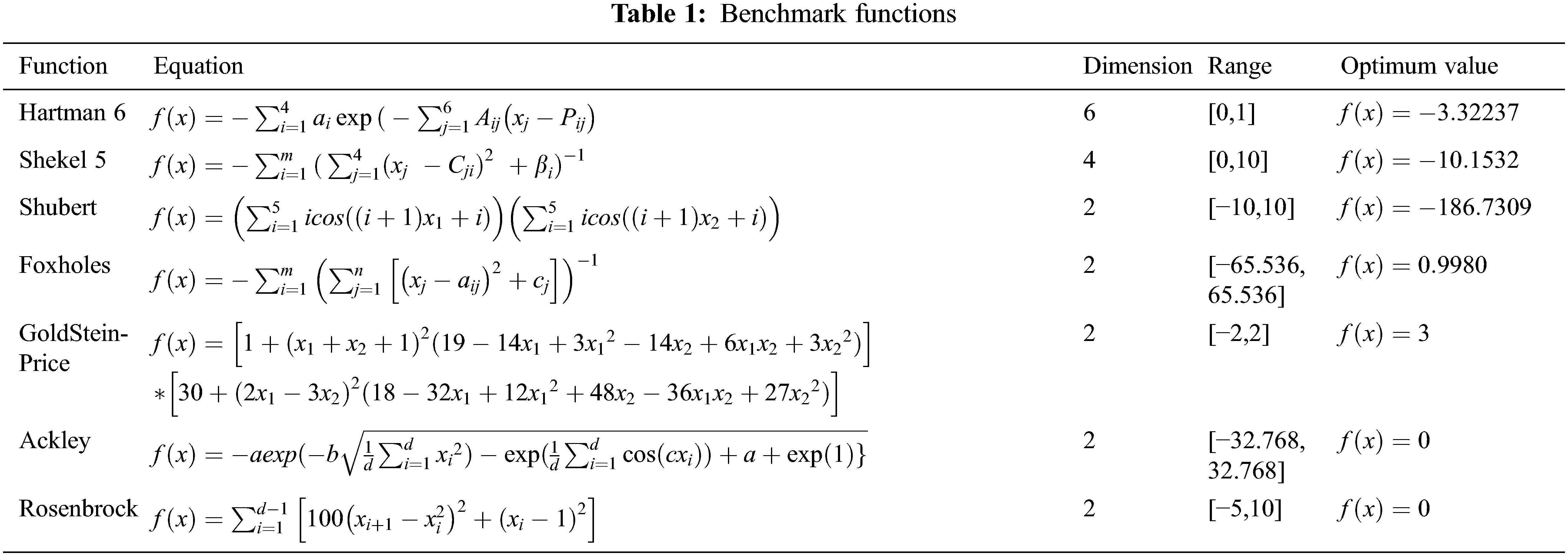
The tests belonging to benchmark test functions shown in Tab. 1 were performed for the five meta-heuristic algorithms in the same conditions. The population of the algorithms was determined as 30. Each was performed 30 times in 200 iterations using Matlab’s R2017b version. Because the objective is to obtain the best outcome with the minimum possible populations and iterations. Additionally, each iteration of the algorithm included a 0.1 s pause. The average result, standard deviation, best result, and average duration values of the study are reported in Tab. 2.

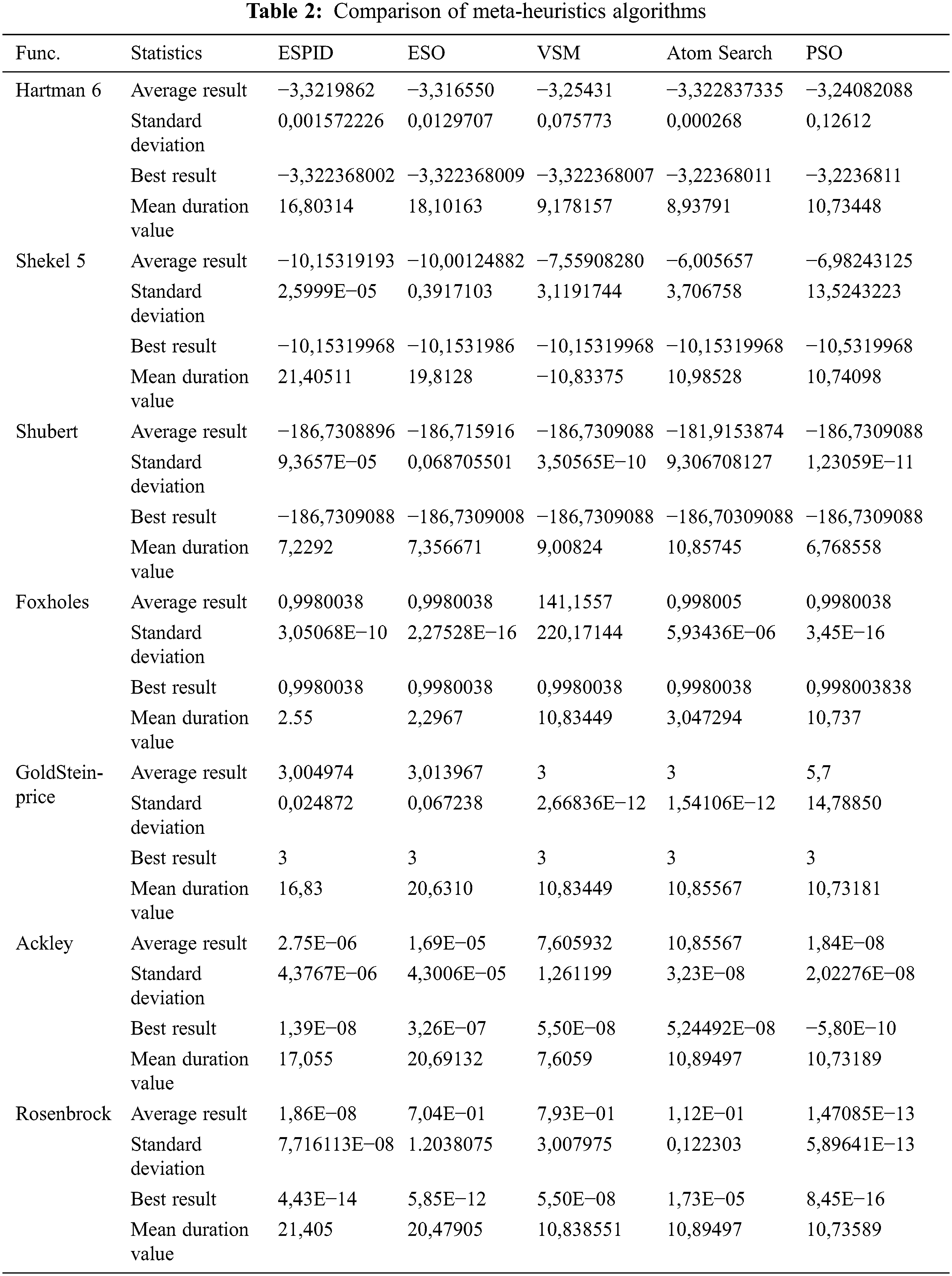
When the ESPID and ESO algorithms were evaluated using the given statistical data, it was determined that ESPID outperformed ESO in terms of the mean and standard deviation values for the Hartman 6, Shubert, GoldStein-Price, Ackley, and Rosenbrock functions (Fig. 8). Additionally, when the mean CPU durations are compared, Tab. 1 shows that the ESPID method converges to the correct result earlier.

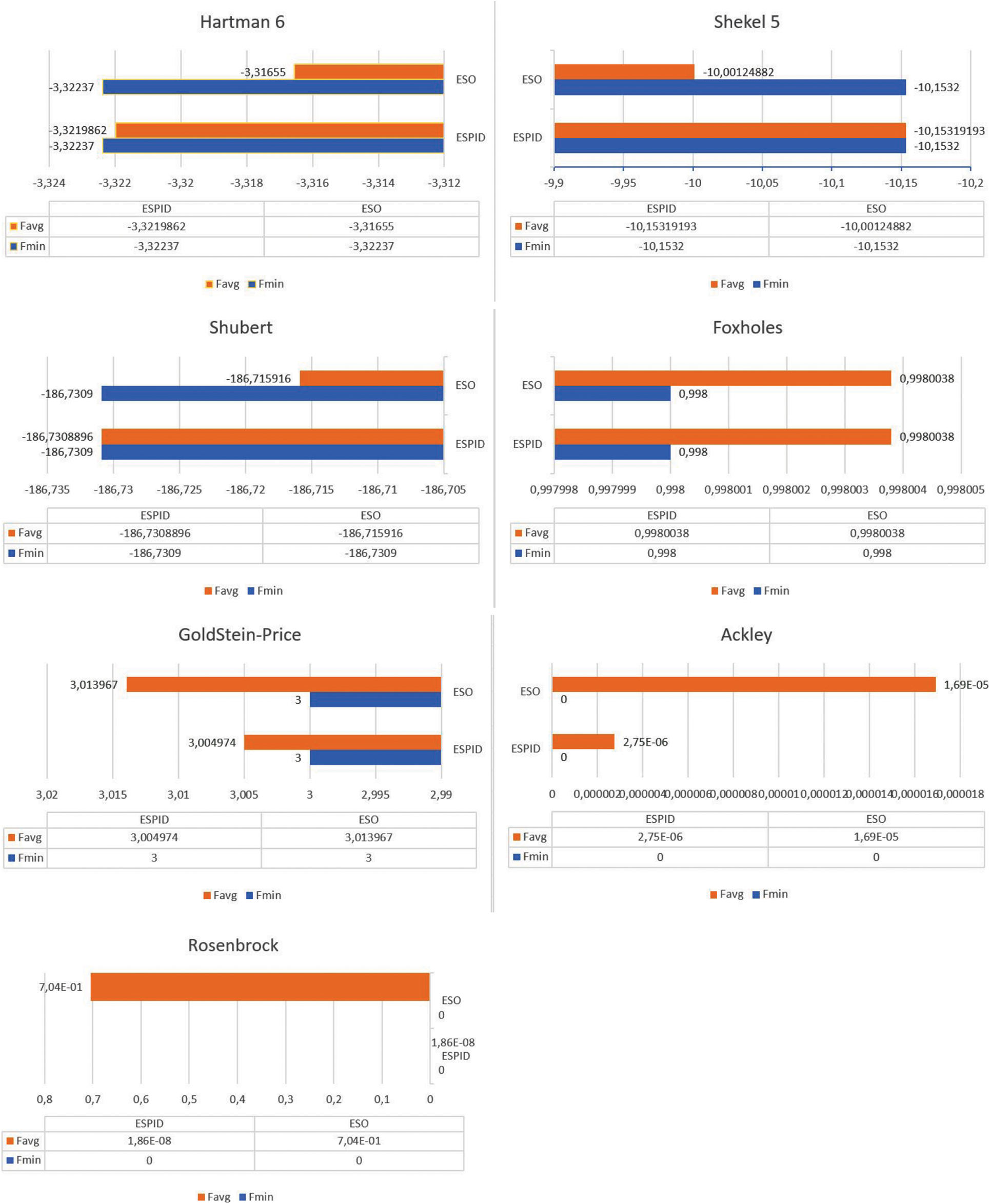
Figure 8: Comparison of mean values of ESO and ESPID algorithms

While examined under the same conditions, the statistical results of these algorithms were compared to the results of the other three meta-heuristic algorithms, namely PSO, Atom Search (ASO), and VSM. As a consequence of the provided population and iteration, it was discovered that all algorithms were unable to achieve the desired result. Even though no algorithm was able to achieve the optimal value of zero in the Rosenbrock and Ackley functions, ESPID algorithms (4,43E−14) and PSO algorithms (8,45E−16) came the closest to achieving the optimal value. In the multidimensional Hartman and Shekel 5 functions, it was discovered that all methods achieved the optimal value at a certain point. When the mean values are considered, however, it can be concluded that the ASO and ESO algorithms provide the worst values. All algorithms reached the best value in the Foxholes function. The ESPID algorithm outperforms the competition in this function, with a mean CPU time of 2,55 s. While VSM and ASO algorithms obtained the optimum mean value of 3 in the GoldStein-Price function, the PSO method had the poorest outcome (See Fig. 9).

Figure 9: Comparison of mean values of ESPID, ESO, VSM, ASO, PSO algorithms

3.1.3 Pressure Vessel Design Problem

In the pressure vessel design problem shown in (Fig. 10), the aim is to minimize the total production cost. There are 4 decision variables in this design. These are body thickness Ts , head thickness Th , inner radius R and section length L [47].

Figure 10: Pressure vessel design problem [47]

x=Ts(x1),Th(x2),R(x3),L(x4) objective function using the design vector [47]:

minf(x)=0,6224x1x3x4+1,778x2x32+3,1661x12x4+19,84x12x3 (25)

The constraints on this objective function are:

g1(x)=−x1+0,0193x3≤0 (26)

g2(x)=−x2+0,009541x3≤0 (27)

g3(x)=−πx32x42−43πx33+1296000≤0 (28)

g4(x)=x4+240≤0 (29)

The simple limits of the problem are 0,0625≤x1,x2≤99 ve 10≤x3,x4≤200 [47].

While applying to the pressure vessel design problem, the population number was determined as 30 and the number of iterations as 2000. Each population was run 30 times. The comparison of the performances of the ESPID algorithm and the ESO algorithm is shown in Tab. 3. When the table is examined, the ESPID algorithm is more successful with the decision variables x1−4=(0.78020,0.39240,40.32340,198.38120) and the lowest cost function value of 5885,452. In addition, when compared with other optimization methods for the pressure vessel design problem in Tab. 4, it has been seen that it is more successful than other methods in terms of worst, average and best values.

4  Conclusions

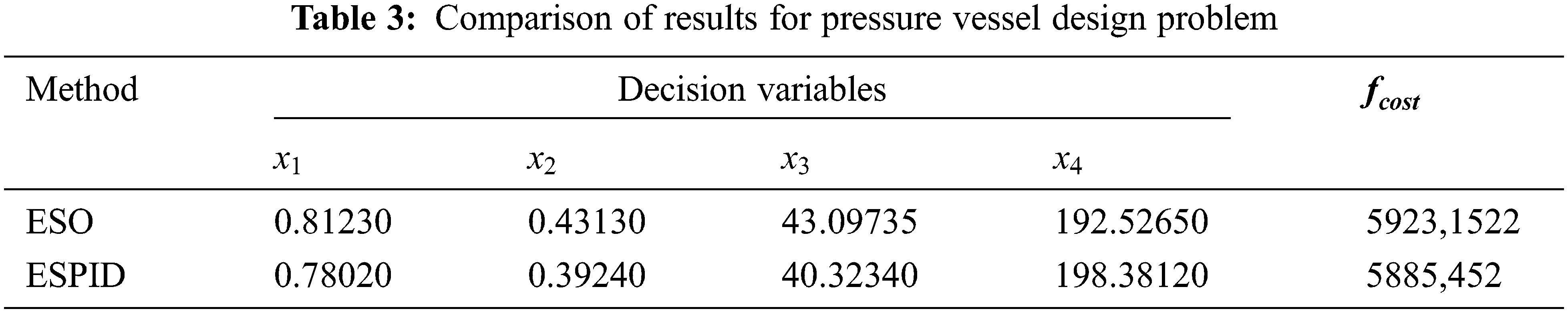
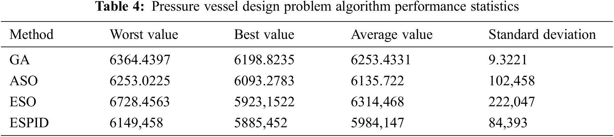
A comparison has been made between the ESO algorithm and ESPID algorithm, which was developed by including an intelligent PID control system rather than the self-tuning orbital-tuner method used in the ESO algorithm. In this comparison, the population of the algorithms was decided to be 30, and the number of iterations was determined as 200. Seven different constrained test functions were applied. After the test was completed, it was discovered that the mean value of the ESPID algorithm performed much better in all functions. Furthermore, when the average durations are taken into account, it can be argued that it produces results faster than the ESO algorithm. When compared to other meta-heuristic algorithms, such as PSO, ASO, and VSM, the ESPID algorithm produced closer results to the benchmark test results. The ESPID algorithm has been applied to the pressure vessel design problem, which is a real-life problem. According to the ESO algorithm, the production cost value gave the least cost with 5885,452. Also, ESPID, when compared to GA, ASO and ESO algorithms, it has the least average production cost with 5984,147 in problem solving.

The performance of the ESPID algorithm in real-life engineering problems can be compared to that of other metaheuristic algorithms in the future.

Funding Statement: The authors received no specific funding for this study.

Conflicts of Interest: The authors declare that they have no conflicts of interest to report regarding the present study.

References

 1.  M. J. Kochenderfer and T. A. Wheeler, Algorithms for optimization. London, England: MIT Press, 2019. [Online]. Available at: https://algorithmsbook.com/optimization/files/optimization.pdf. [Google Scholar]

 2.  E. Hazan, “Introduction to online convex optimization,” Foundations and Trends in Optimization, vol. 2, no. 3–4, pp. 157–325, 2015. [Google Scholar]

 3.  Y. Xue, J. Jiang, B. Zhao and T. Ma, “A self-adaptive artificial bee colony algorithm based on global best for global optimization,” Soft Computing, vol. 22, no. 9, pp. 2935–2952, 2018. [Google Scholar]

 4.  G. Dhiman, K. K. Singh, A. Slowik, V. Chang, A. Yildiz et al., “EMoSOA: A new evolutionary multi-objective seagull optimization algorithm for global optimization,” International Journal of Machine Learning and Cybernetics, vol. 12, no. 2, pp. 571–596, 2021. [Google Scholar]

 5.  A. R. Yildiz, “Taşıt elemanlarının yapısal optimizasyon teknikleri ile optimum tasarımı,” Politeknik Dergisi, vol. 20, no. 2, pp. 319–323, 2017. [Google Scholar]

 6.  M. Gendreau and J. Y. Potvin, Handbook of metaheuristics, vol. 2, New York, USA: Springer, pp. 9, 2010. [Google Scholar]

 7.  G. G. Wang, S. Deb and Z. Cui, “Monarch butterfly optimization,” Neural Computing and Applications, vol. 31, no. 7, pp. 1995–2014, 2019. [Google Scholar]

 8.  A. Tabari and A. A. Arshad, “New optimization method: Electro-Search algorithm,” Computers & Chemical Engineering, vol. 103, pp. 1–11, 2017. [Google Scholar]

 9.  R. L. Haupt and S. E. Haupt, Practical Genetic Algorithms, New Jersey, USA: John Wiley & Sons, pp. 253, 2004. [Google Scholar]

10. J. Kennedy and R. Eberhart, “Particle swarm optimization,” in Proc. ICNN’95-Int. Conf. on Neural Networks, Perth, WA, Australia, pp. 1942–1948, 1995. [Google Scholar]

11. K. N. Krishnanand and D. Ghose, “Detection of multiple source locations using a glow worm metaphor with applications to collective robotics,” in Proc. IEEE Swarm Intelligence Symp., Pasadena, CA, USA, pp. 84–91, 2005. [Google Scholar]

12. A. K. M. Passino, “Biomimicry of bacterial foraging for distributed optimization and control,” IEEE Control System Magazine, vol. 22, no. 2, pp. 52–67, 2002. [Google Scholar]

13. W. Zhao, L. Wang and Z. Zhang, “A novel atom search optimization for dispersion coefficient estimation in groundwater,” Future Generation Computer Systems, vol. 91, no. 4, pp. 601–610, 2019. [Google Scholar]

14. P. A. Castillo, M. G. Arenas and N. Rico, “Determining the significance and relative importance of parameters of a simulated quenching algorithm using statistical tools,” Applied Intelligence, vol. 37, no. 2, pp. 239–254, 2012. [Google Scholar]

15. A. Alfi, “PSO with adaptive mutation and inertia weight and its application in parameter estimation of dynamic systems,” Acta Automatica Sinita, vol. 37, no. 5, pp. 541–549, 2011. [Google Scholar]

16. H. Abubakr, T. H. Mohamed, M. M. Hussein and G. Shabib, “ESO-based self-tuning frequency control design for isolated microgrid system,” in Proc. 2019 21st Int. Middle East Power Systems Conf. (MEPCON), Cairo, Egypt, pp. 589–593, 2019. [Google Scholar]

17. N. M. Tabatabaei, S. R. Mortezaei, S. Shargh and B. Khorshid, “Solving multi-objective optimal power flow using multi-objective electro search algorithm,” International Journal on Technical and Physical Problems of Engineering (IJTPE), vol. 9, pp. 1–8, 2017. [Google Scholar]

18. Y. A. Dahab, H. Abubakr and T. H. Mohamed, “Adaptive load frequency control of power systems using electro-search optimization supported by the balloon effect,” IEEE Access, vol. 8, pp. 7408–7422, 2020. [Google Scholar]

19. M. Yazandost, P. Khazaei, S. Saadatian and R. Kamali, “Distributed optimization strategy for multi area economic dispatch based on electro search optimization algorithm,” in Proc. 2018 World Automation Congress (WAC), Stevenson, WA, USA, pp. 1–6, 2018. [Google Scholar]

20. J. Cavazos, J. E. B. Moss and M. F. P. O’Boyle, “Hybrid optimizations: Which optimization algorithm to use?,” in Compiler Construction, In: A. Mycroft, A. Zeller (Eds.Berlin, Heidelberg, 2006, https://link.springer.com/book/10.1007/11688839 [Google Scholar]

21. J. Pan, N. Liu, S. C. Chu and T. Lai, “An efficient surrogate-assisted hybrid optimization algorithm for expensive optimization problems,” Information Sciences, vol. 561, no. 2, pp. 304–325, 2021. [Google Scholar]

22. S. Velliangiri, P. Karthikeyan, A. Xavier and D. Baswaraj, “Hybrid electro search with genetic algorithm for task scheduling in cloud computing,” Ain Shams Engineering Journal, vol. 12, no. 1, pp. 631–639, 2021. [Google Scholar]

23. M. F. Esa, N. H. Mustaffa and N. H. Mohamed Radzi, “A hybrid algorithm based on flower pollination algorithm and electro search for global optimization,” International Journal of Innovative Computing, vol. 8, no. 3, pp. 81–88, 2018. [Google Scholar]

24. U. Kose and O. Deperlioglu, “Electro-Search algorithm and autoencoder based recurrent neural network for practical medical diagnosis,” in Proc. 2019 Innovations in Intelligent Systems and Applications Conf. (ASYU), Izmir, Turkey, pp. 1–6, 2019. [Google Scholar]

25. J. A. Marmolejo Saucedo, J. D. Hemanth and U. Kose, “Prediction of electroencephalogram time series with electro-search optimization algorithm trained adaptive neuro-fuzzy inference system,” IEEE Access, vol. 7, pp. 15832–15844, 2019. [Google Scholar]

26. Y. Song, X. Huang and C. Wen, “Robust adaptive fault-tolerant PID control of MIMO nonlinear systems with unknown control direction,” IEEE Transactions on Industrial Electronics, vol. 64, no. 6, pp. 4876–4884, 2017. [Google Scholar]

27. S. Ekinci and B. Hekimoglu, “Improved kidney-inspired algorithm approach for tuning of PID controller in AVR system,” IEEE Access, vol. 7, pp. 39935–39947, 2019. [Google Scholar]

28. W. Chang and S. Shih, “PID controller design of nonlinear systems using an improved particle swarm optimization approach,” Communications in Nonlinear Science and Numerical Simulation, vol. 15, no. 11, pp. 3632–3639, 2010. [Google Scholar]

29. B. Farnad, A. Jafarian and D. Baleanu, “A new hybrid algorithm for continuous optimization problem,” Applied Mathematical Modelling, vol. 55, no. 7–8, pp. 652–673, 2018. [Google Scholar]

30. K. Tang, X. Yao, P. N. Suganthan, C. Macnish, Y. P. Chen et al., “Benchmark functions for the CEC’2008 special session and competition on large scale global optimization,” Nature Inspired Computation and Applications Laboratory, vol. 24, pp. 1–18, 2007. [Google Scholar]

31. B. Chen, R. Kuhn and G. Foster, “Vector space model for adaptation in statistical machine translation,” in Proc. Proc. of the 51st Annual Meeting of the Association for Computational Linguistics, Sofia, Bulgaria, pp. 1285–1293, 2013. [Google Scholar]

32. R. P. Borase, D. K. Maghade and S. Y. Sondkar, “A review of PID control, tuning methods and applications,” International Journal of Dynamic and Control, vol. 9, no. 2, pp. 818–827, 2021. [Google Scholar]

33. K. H. Ang, G. Chong and Y. Li, “PID control system analysis, design, and technology,” IEEE Transactions on Control Systems Technology, vol. 13, no. 4, pp. 559–576, 2005. [Google Scholar]

34. A. B. Sharkawy, “Genetic fuzzy self-tuning PID controllers for antilock braking systems,” Engineering Applications of Artificial Intelligence, vol. 23, no. 7, pp. 1041–1052, 2010. [Google Scholar]

35. Z. Xiang, D. Ji, H. Zhang, H. Wu and Y. Li, “A simple PID-based strategy for particle swarm optimization algorithm,” Information Sciences, vol. 502, no. 10, pp. 558–574, 2019. [Google Scholar]

36. G. Zeng, X. Xie, M. Chen and J. Weng, “Adaptive population extremal optimization-based PID neural network for multivariable nonlinear control systems,” Swarm and Evolutionary Computation, vol. 44, no. 4, pp. 320–334, 2019. [Google Scholar]

37. Q. Sun, C. Du and Y. Duan, “Design and application of adaptive PID controller based on asynchronous advantage actor-critic learning method,” Wireless Network, vol. 27, no. 5, pp. 3537–3547, 2021. [Google Scholar]

38. T. Xiang, X. Liao and K. Wong, “An improved particle swarm optimization algorithm combined with piecewise linear chaotic map,” Applied Mathematics and Computation, vol. 190, no. 2, pp. 1637–1645, 2007. [Google Scholar]

39. T. S. Kemmoe and M. Gourgand, “Particle swarm optimization: A study of particle displacement for solving continuous and combinatorial optimization problems,” International Journal of Production Economics, vol. 121, no. 1, pp. 57–67, 2009. [Google Scholar]

40. M. Clerc and J. Kennedy, “The particle swarm-explosion, stability, and convergence in a multidimensional complex space,” IEEE Transactions on Evolutionary Computation, vol. 6, no. 1, pp. 58–73, 2002. [Google Scholar]

41. A. Bigham and S. Gholizadeh, “Topology optimization of nonlinear single-layer domes by an improved electro-search algorithm and its performance analysis using statistical tests,” Structural Multidisciplinary Optimization, vol. 62, pp. 1821–1848, 2020. [Google Scholar]

42. I. Coskun and H. Terzioglu, “Hız performans eğrisi kullanılarak kazanç(PID) parametlerinin belirlenmesi,” Selcuk University Journal of Engineering Sciences, vol. 6, no. 3, pp. 180–205, 2007. [Google Scholar]

43. S. K. Nie, Y. J. Wang, S. Xiao and Z. Liu, “An adaptive chaos particle swarm optimization for tuning parameters of PID controller,” Optimal Control Applications and Methods, vol. 38, no. 6, pp. 1091–1102, 2017. [Google Scholar]

44. M. Kishnani, S. Pareek and R. Gupta, “Optimal tuning of PID controller by Cuckoo Search via Lévy flights,” in Proc. 2014 Int. Conf. on Advances in Engineering & Technology Research (ICAETR, Unnao, India, pp. 1–5, 2014. [Google Scholar]

45. A. A. M. Zahir, S. S. N. Alhady, W. A. F. W. Othman and M. F. Ahmad, “Genetic algorithm optimization of PID controller for brushed DC motor,” in Intelligent Manufacturing & Mechatronics. Lecture Notes in Mechanical Engineering. Singapore: Springer, 2018. [Online]. Available at: https://link.springer.com/chapter/10.1007/978-981-10-8788-2_38. [Google Scholar]

46. M. Jamil and X. S. Yang, “A literature survey of benchmark functions for global optimisation problems,” International Journal of Mathematical Modelling and Numerical Optimisation, vol. 4, no. 2, pp. 150–194, 2013. [Google Scholar]

47. A. Tran, M. Tran and Y. Wang, “Constrained mixed-integer Gaussian mixture Bayesian optimization and its applications in designing fractal and auxetic metamaterials,” Structural and Multidisciplinary Optimization, vol. 59, no. 6, pp. 2131–2154, 2019. [Google Scholar]