Multiobjective Economic/Environmental Dispatch Using Harris Hawks Optimization Algorithm

Nomenclature

1  Introduction

The significance of Economics Dispatch (ED) is remarkably high in the power systems since it aims to minimalize fuel expenditure while compensating system constraints by scheduling the output of all available generating units in the power system and hence the recent developments in the power generating sectors have prioritized the process of ED in a wider range [1,2]. The process of resolving the ED issue is used to optimize the usage of fossil fuels in thermal making unit for satisfying the demand while providing the electric power [3]. While trying to solve Emission Dispatch as a single objective function, the corresponding cost gets increased [4]. The single objective ED problem is resolved by treating the emission of Nitrogen oxides (NOx), Sulfur oxides (SOx) as constraints [5]. This emission constraint ED problem is remarkably solved by various researches in [6,7]. Furthermore, the Combined EED (CEED) problem is resolved as a single objective issue through the price penalty factor [8] and weighted sum method [9]. However, these methods are not capable enough to attain the optimal outcome from the non-convex Pareto optimal front since it necessitates multiple runs. To overcome this drawback, the Multi-Objective EED (MOEED) issue is rectified simultaneously as a conflicting objective function.

Over the past few years, multi-objective evolutionary algorithm is used for resolving this problem. Several solution approaches [10–14] are introduced to solve the MOEED problem by producing multiple Pareto optimal solution from a single run.

While integrating thermal generating unit with renewable resources, wind energy is highly feasible since it owns multiple beneficial impacts including low production cost. Initially, the investigators have predicted the future wind speed by employing different approaches like fuzzy logic approach [15], neural network [16], time series model [17]. Hetzer [18] and solved the ED problem in an optimal manner.

The motive of this work is to sort out the MOEED problem with the aid of the newly formulated population-based HHO algorithm, which is capable enough to solve these issues with plenty of advantageous impacts like less complexity, maximal accuracy, simple mechanism, optimal optimization output and randomness. The usage of long-term memory approach aids the convergence characteristics of HHO algorithm by narrowing down the search space. The non-dominated solution set is maintained using the crowding distance method and the fuzzy based methodology is implemented to find the compromising solution. The attained results are compared with various literature papers to prove the efficiency of the work. In addition, a wind energy conversion system is also included with same problem and the results are displayed.

The remaining part of this paper includes modelling of Wind Energy Conversion System (WECS) in Section 2, Formulation of EED problem in Section 3, description of HHO in Section 4, updating process of long term memory in Section 5, description of External Repository Updating Strategy in Section 6, Finding of compromise solution in Section 7, the selection of best Compromise Solution in Section 8, Result analysis in Section 9 and conclusion in Section 10.

2  Modelling and Analysis of WECS

In nature, the wind speed v(ms) is a random variable. The wind speed’s output power is assumed as a piece wise linear function and it can be modelled for a v  based on the power characteristics zones of wind energy conversion system as [19],

PW(v)={0v<vin,v>voPWrv−vinvr−vinvin≤v≤vrPWrvr≤v≤vo (1)

The transformed wind power is stochastic in nature [20]. Since the wind power is a discrete variable in the zones ([ v<vin,v>vo],[≤v≤vo] ) it can be represented by cumulative distribution function. As the wind power is linear and continuous in (vin≤v≤vr), probability density function is employed to represent the output wind power.

Probability of wind power being zero:

PrW(PW=0)=PrW(v<vin)+PrW(v>vo)=1− exp[−(vinc)k]+exp[−(voc)k] (2)

Probability of rated wind power:

PrW(PW=PWr)=PrW(vr≤v≤vo)exp[−(vrc)k]−exp[−(v0c)k]

Probability of wind power in continuous zone ( 0≤PW≤PWr )

fPW(PW)=(khvincPWr)[(1+hPWPWr)vinc]×exp{−[(1+hPWPWr)vinc]k} (3)

h=(vr−vin)vin

2.1 Operational Cost of Available Wind Generator

The operating cost of wind power can be modelled as,

F(PW)=∑j=1M⁡F(PWj)

=∑j=1M⁡Fd,wj(PWj,sc)+∑j=1M⁡Fr,wj(PWj,sc−PWj,av)+∑j=1M⁡Fp,wj(PWj,av−PWj,sc) (4)

It consists of three parts. The first part gives the direct cost of wind generators. If the operator has owned the wind farm then this part becomes zero. Else the operator should pay the direct amount to the owner. The direct cost operation is proportional to the scheduled wind power, which is expressed as

Fd,wj(PWj,sc)=kd,wj.PWj,sc (5)

The second part of the equation denotes wind generator’s reserve or overestimation cost. When the prevailing wind energy is insufficient to satisfy the demand, this term can be modelled as,

Fr,wj(PWj,sc−PWj,av)=kr,wj∫0PWj,sc⁡(PWj,sc−PWj)fPW(PWj) dpw (6)

The third term of the equation is the penalty cost or underestimation cost. When the prevailing wind power is excess than the demand this can be modelled as,

Fp,wj(PWj,av−PWj,sc)=kp,wj∫PWj,avPWj⁡(PWj−PWj,av)fPW(PWj) dpw (7)

3  EED Problem Formulation

The EED includes certain issues like limited Generator capacity, losses in network transition, ramp rate limits and restricted operating zone, which are effectively rectified with the assistance of the introduced optimization approach. By meeting system limitations, the traditional EED issue concurrently lessens the fuel price and ED of thermal units. The constraints and the objective processes are specified in the subsequent section.

3.1 Objective Function1: Minimization of Total Cost

F(PG)=∑i=1NG⁡ai+biPGi+ciPGi2 (8)

The overall cost of the ED issue is actually the sum of the wind generator’s operational cost and the thermal unit’s fuel cost.

FT= F(PG)+ F(PW) (9)

3.2 Objective Function2: Minimization of Emission Dispatch

E(PG)=∑i=1NG⁡10−2(αi+βiPGi+γiPGi2)+ηiexpδi (10)

3.3 Overall Objective Function of EED Problem

The multi-objective, constrained EED issue can be formulated with wind generator is given by,

Minimize {FT,E(PG)}

Subject to

Power balance constraints:

∑i=1NG⁡PGi=PDemand+Ploss (11)

where,

Ploss=∑i=1NG⁡∑j=1NG⁡PGiBijPGj+∑i=1NG⁡B0iPGi+B00

Generation capacity constraint

For thermal unit PGimin≤PGi≤PGimax

For wind generator 0≤PWj≤PWrj

4  Harris Hawks Optimization

The author developed a mathematical model using chasing and hunting process of harris hawks and proposed a population based, nature inspired optimization problem [21]. The cooperative hunting style of these hawks includes monitoring, approaching, encircling and attacking the prey. Harris hawks perform the Leapfrog motion whereas they occasionally re-joining and splitting again for the hunting process. The “surprise pounce”, which is otherwise recognized as the “seven kills” approach is the major tactic used by these hawks to catch the prey. According to the developers, exploration and exploitation phases are carried out with perching and besieging process. The pseudo code for HHO is given below:

Inputs: Hawks size N, total number of iterations T, size of memory location K

Output: best position of the rabbit and its fitness value

Set the position of each Hawks

While (the termination condition is fulfilled (t<T) ) do

Compute the fitness value of each Hawks

Set the position of rabbit Xrabbitt as the best position among Z number of Hawks

Update memory location with Xrabbitt

For each hawk ( Xi) do

Calculate the escaping energy (E) of the rabbit using

E=2E0(1−tT)

if |E|≥1 /*exploration phase

update the position of hawks ( Xi) using

X(t+1)={Xr(t)−r1|Xr(t)−2r2X(t)|q≥0.5(Xt(t)−Xm(t))−r3(LB+r4(UB−LB))q<0.5

end if

if |E|<1 /*exploitation phase

Set a random number r from 0 to 1

if ( r≥0.5and|E|≥0.5) /*soft besiege

update hawks location ( Xi) using

X(t+1)=ΔX(t)−E|J(Xt(t)−X(t)|

ΔX(t)=(Xt(t)−X(t)

else if ( r≥0.5 and |E|<0.5 ) /* hard besiege

update hawks location ( Xi) using

X(t+1)=Xt(t)−E|ΔX(t)|

else if ( r<0.5 and |E|≥0.5 ) /* softbesiegewithrapiddives

update the position of hawks ( Xi) using

Y=Xt(t)−E|J(Xt(t)−X(t)|

X(t+1)={YifF(Y)<F(X(t))ZifF(Z)<F(X(t))

else if ( r<0.5 and |E|<0.5 ) /* hardbesiegewithrapiddives

update the position of hawks ( Xi) using

X(t+1)={YifF(Y)<F(X(t))ZifF(Z)<F(X(t))

end if

end for

end while

Return Xrabbit

5  Long Term Memory Updating Process in HHO

In hunting strategies of HHO the position of each hawks can be updated based on the single best position Xt(t) of the targeted prey. In some cases, it may lead to premature convergence. To overcome this issue the Memory Location (ML) concept is implemented to store the consecutive best position of targeted prey in every iteration. The size of ML is made by several trials. The ML is updated based on first in-first out concept. In each iteration of HHO, the latest optimal position of the prey replaces the old location. After updating the position of the hawks in each iteration the best position of the targeted prey is chosen using the probability Pi

Pi=fitnessofXti∑k=1ML⁡fitnessofXtk (12)

After calculating the probability for each best position of the prey in ML, the selection process is carried out using Roulette Wheel Selection method. During each iteration the size of ML should be maintained constant.

The entire process of ML is depicted in the Fig. 1. Let l be the size of the ML. The best position till lth iteration is occupied in ML. After l+1th iteration the oldest best position can be replaced by the new best position in ML. This process is continued for the entire hunting process.

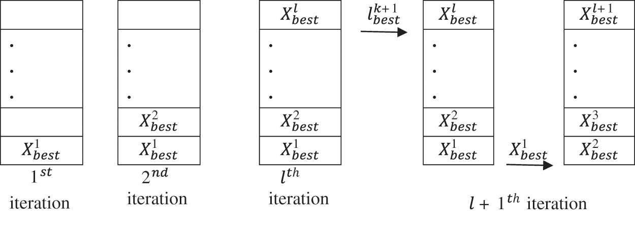
Figure 1: Memory updating process

6  External Repository Updating Strategy

The selection of promising individual for the next iteration is based on the dominance relation. The new feasible solution ( x1) allows to take a position in external repository controller (archive controller). The position of x1 can be hold based on the dominance relation with the upcoming solutions xn,{i=2,3 . . .N} . The updating process of archive is fall under the below cases,

Case 1: At initial stage the A/ (archive) is empty. The new feasible solution ( x1) is allowed to take a position in the A/ . It becomes xgA/

Case 2: If the incoming solution  xn,{i=2,3 . . .N}⪯∃{g=1,2,. . . G}xgA/ : where G represent the size of A/ , then xgA/→xn .

Case 3: If ∃{g=1,2,. . . G}xgA/ ∼⪯xn,{i=2,3 . . .N} , then A/ allocate a position to xn .

Case 4: ∃{g=1,2,. . . G}xgA/ ⪯xn,{i=2,3 . . .N} , then A/ remains unchanged.

Finally, the dominant solutions take a position in the archive controller. The solutions in the controller are non-dominating to each other. This strategy effectively increases the global search mechanism.

7  External Repository Maintaining Strategy

It is required to maintain the size of external repository in every iteration. If the size exceeds the fixed value, the exceeded solutions can be removed by considering the crowding distance. This distance is computed for each solution based on neighboring solutions. The solutions having minimum crowding distance is removed from the repository to maintain the size of the repository.

7.1 Pseudo Code for Maintaining the Size of Repository

A/new= function_name ( A/updated,NA/)

Na=size(A/updated,1)

if    Na >NA/

/* initialize crowding distance as zero*/

CD(A/j=1:NA/updated)=0;

for i=1 to k do

/*sorting the members of A/updated based on the ith fitness function*/

SA/updated=sort(A/updated,i) ;

/* assign inf for first and last members in SA/updated */

SA/1updated=inf;

SA/Naupdated=inf;

/* calculate CD between the 2nd and the previous last member */

for j=2 to Na−1 do

CD(A/jupdated)=CD(A/jupdated)+(SA/j−1updated−SA/j+1updated)(max(A/updated)−min(A/updated))

end for

/* sort the CD from minimum to maximum and store the index value in I */

[∼,I]=sort(CD(A/jupdated),ascend)

/* calculate the excess number of solutions in A/updated */

Ne=Na−NA/

/* delete Ne number of solutions from the A/updated */

A/I→1:Neupdated=[ ];

end if

returnA/new←A/updated

8  Compromise Solution Selection Using Fuzzy Based Theory

To get at the ideal solution, the best compromise option has to be picked from the solution set. Here the selection process is done based on the fuzzy membership approach, which is significantly illustrated in Fig. 2. The membership value of each individual j for objective function i is given by

μij={1fi<fiminfimax−fifimax−fiminfimin<fi<fimax0fi>fimax (13)

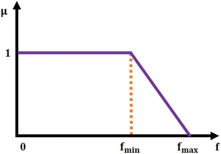
Figure 2: Fuzzy membership function

where  fiminandfimax, denote the minimumandmaximumvaluesofith objective function whereas l gives the amount of non-dominated solution.

The normalized membership value for j is given by

μj=∑i=1k⁡μij∑j=1l⁡∑i=1k⁡μij (14)

The solution which has the high membership value i.e., max{μj ;j=1,2 , . . . . . l} will be chosen as the best non dominated solution.

9  Results and Discussion

The details of transmission losses, coefficients of fuel price and emission are referred from [18]. The system demand is taken as 2.834MW . The coding is developed in MATLAB. To analyze the result more effectively three cases were considered here

Case1: To analogize the extreme and compromise solutions with the existing methods, HHO is applied to IEEE 30 bus, 6 generator system. The system is assumed to be lossless.

Case 2: The solution quality of the HHO algorithm is analyzed using performance evaluation indices like SP, HV and CM with the well-known Particle Swam Optimization (PSO) by handling the system with losses.

Case 3: The performance indices of the HHO algorithm is analogized with PSO including wind power.

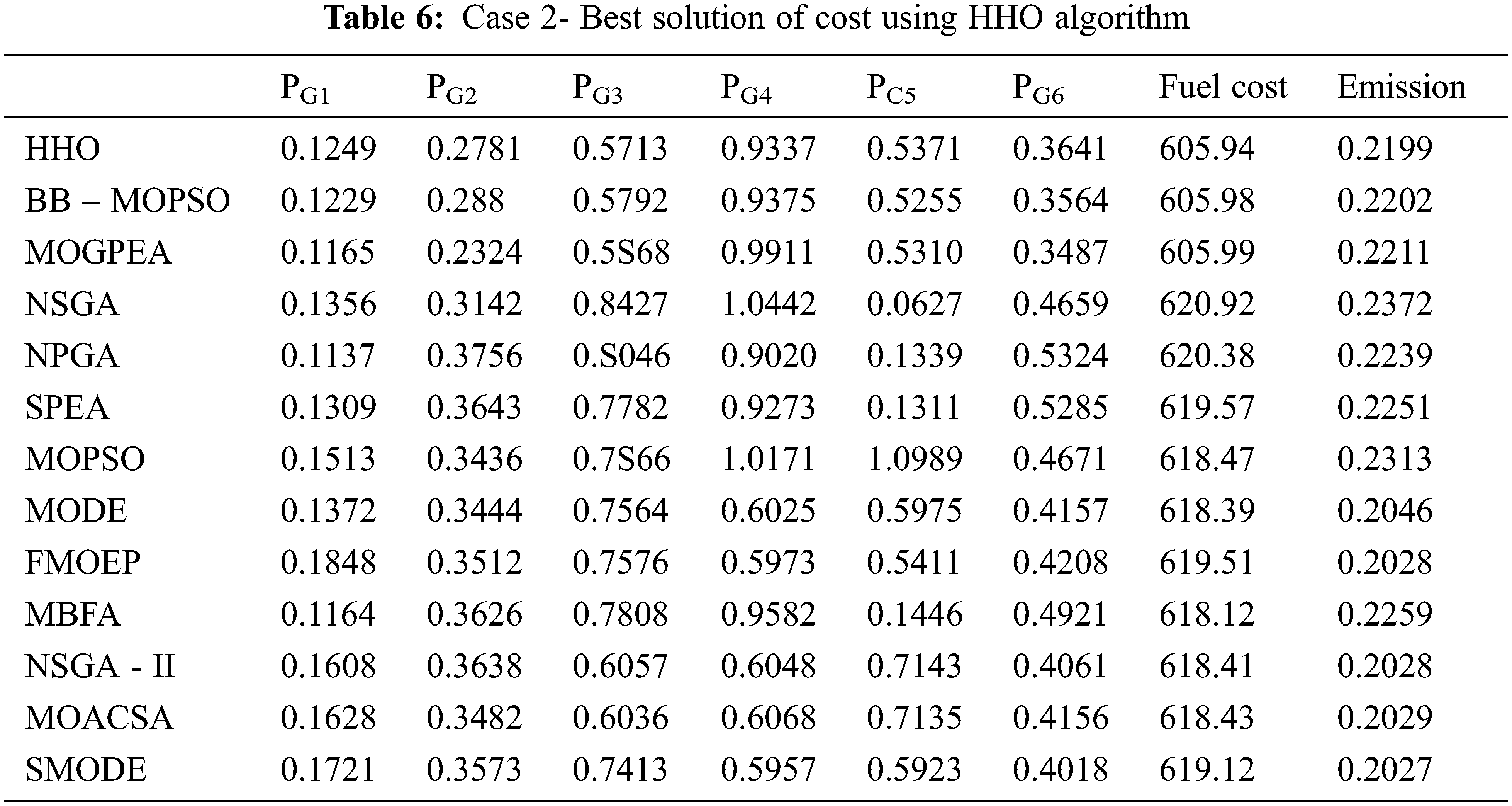
9.1 Case1: Comparative of Extreme and Compromising Solution

Initially, the HHO algorithm is applied to MOEED problem to obtain the maximum solutions. The MOEED dispatch issue is considered as a single objective issue with emission dispatch or fuel cost to find the optimized value of emission dispatch and minimum fuel cost.

Here, Number of Hawks N = 30, Size of Achieve N_ A/  = 30, Size of Memory Location l = 10, maximum no of iterations T = 500. The best cost ($/h) and ED (ton/h) is depicted in Tab. 1. The convergence characteristics are portrayed in Fig. 3. Tab. 2 validates that the optimal fuel cost is and the optimal ED is 0.1942(ton/h) . The extreme solution of fuel expenditure and ED is compared with the results from various literatures [12] like Niched Pareto Genetic Algorithm (NPGA), Non-Dominated Sorting Genetic Algorithm-II (NSGA-II), FMOEP, Strength Pareto Evolutionary Algorithm (SPEA), Modified Bacterial Foraging Algorithm (MBFA), Multiobjective Adaptive Clonal Selection Algorithm (MOACSA), NSGA, Multiobjective Grey Prediction Evolutionary Algorithm (MOGPEA), Summation Based Multiobjective Differential Evolution Algorithm (SMODE) and MOPSO in Tabs. 3 & 4.

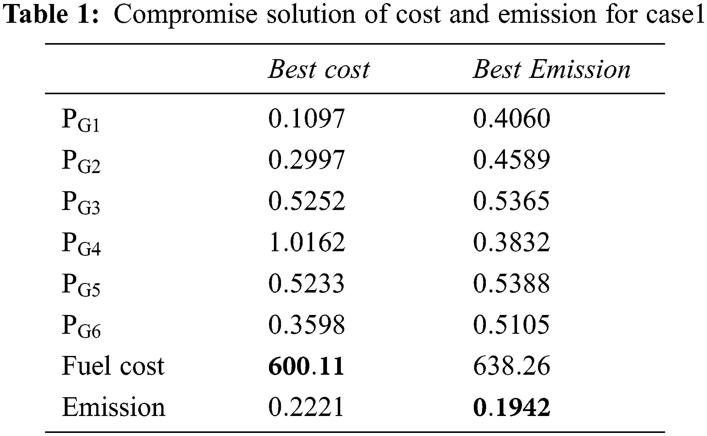
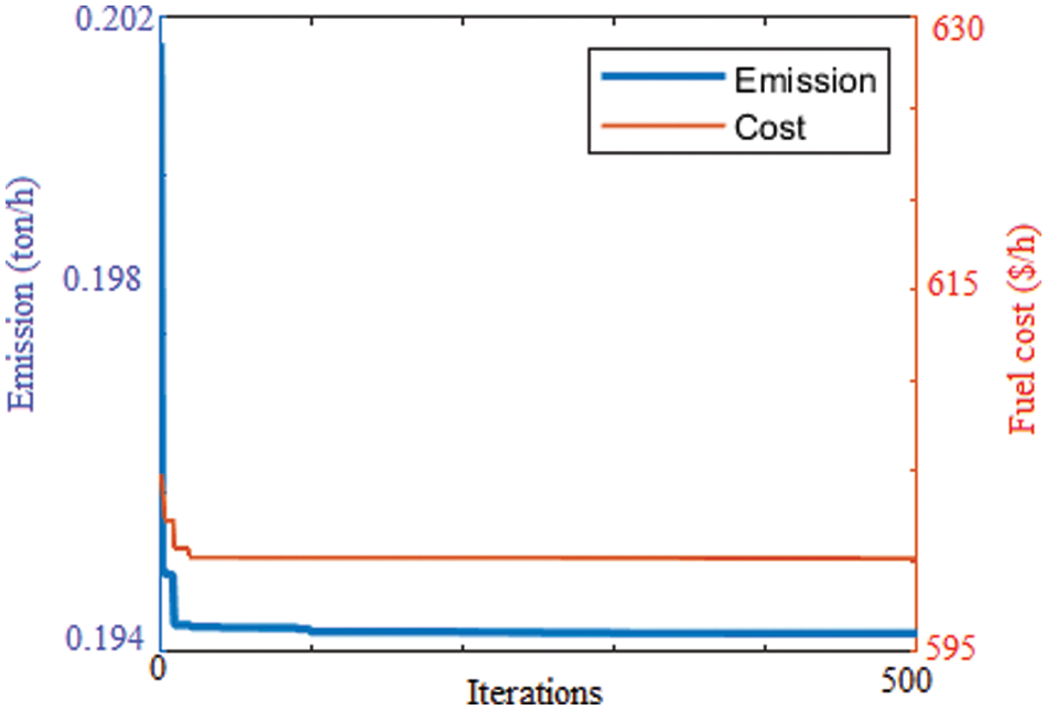
Figure 3: Convergence curve of cost and emission for case1

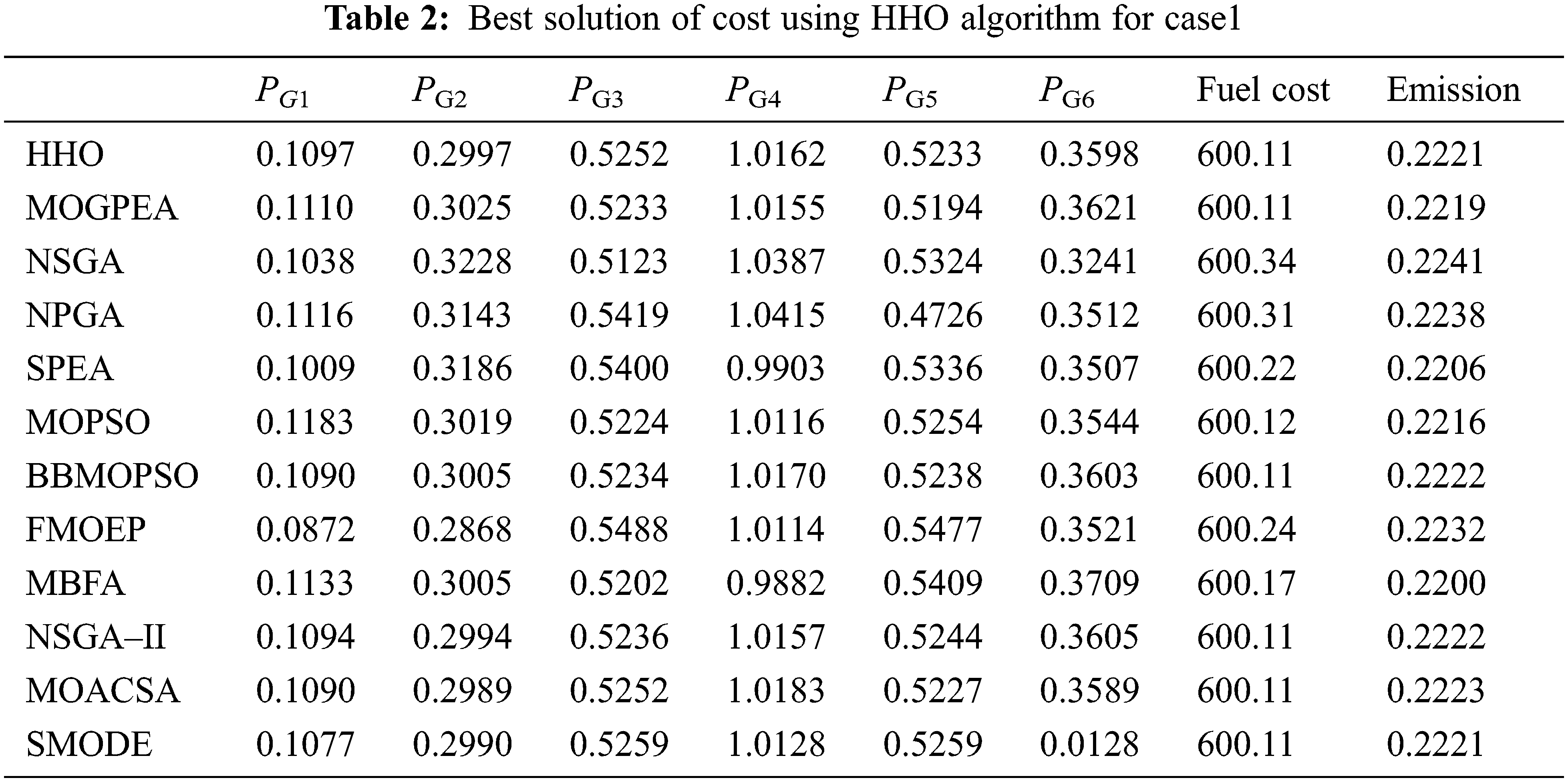
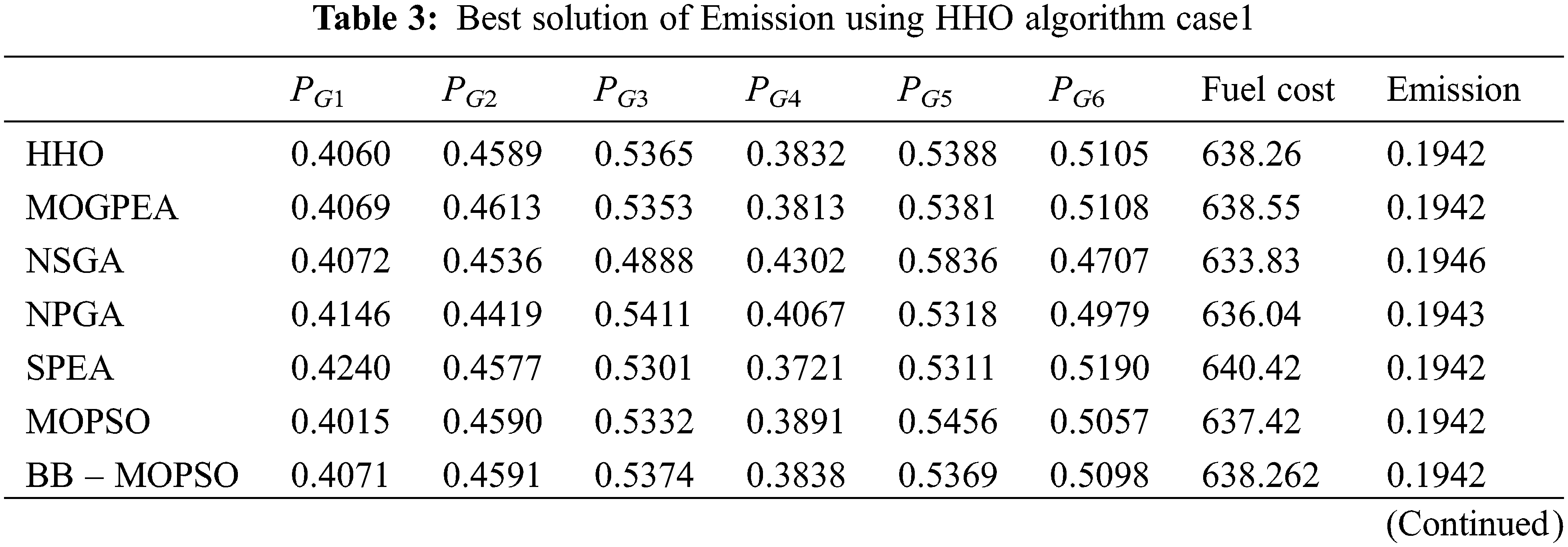
In case of fuel cost HHO produces the optimum value of 600.11 $/h, which is same as the value obtained from NSGA II, MOACSC, MOGPEA, BB- SMODE and MOPSO. HHO produces better results when compared to FMOEP, NPGA, NSGA, MBFA and MOPSO. The corresponding emission value got improvised than NPGA, FMOEP, NSGA-II and MOACSC. It produces the optimum emission value of 0.1942 ton/h which is same as the results in SPEA, FMOEP, BB-MOPSO, MBFA, NSGA-II, MOPSO, MOGPEA whereas it performs better than NPGA and NSGA.

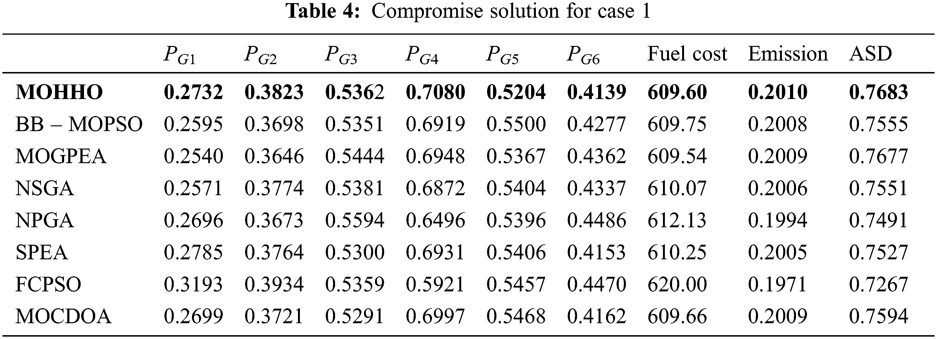
In addition, the HHO is instigated to regulate the fuel expenditure and ED, which is depicted in Fig. 4. For analogizing the compromise solution with the literature results, Average Satisfactory Degree (ASD) is calculated. Tab. 4 shows that the HHO produces the best ASD (=0.7683) value among the various algorithm reported in literature. Even though it gives high emission dispatch, it proves its efficiency in optimum fuel cost of 609.60 ($/h), which is the ideal compromising solution obtained so far.

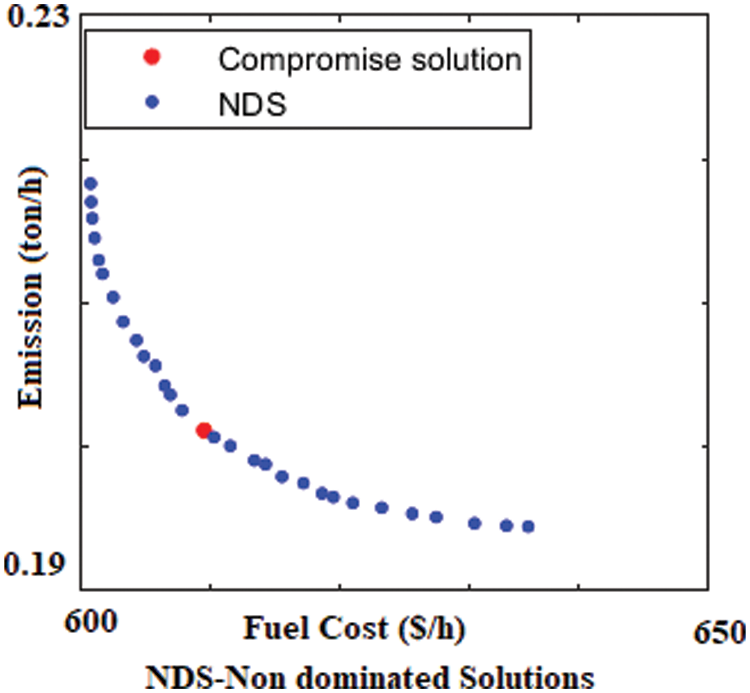
Figure 4: NDS-Non dominated solution of HHO for case 1

Case 2: In this case the algorithm is made to run with the population size of N T = 50 and the maximum iteration is T = 1000. The obtained results of best fuel cost and emissions are specified in Tabs. 6 & 7. These outcomes are analogized with other algorithms like SMODE, FMOEP, SPEA, BB-MOPSO, NSGA II, MOGPEA, MBFA, NSGA, MODE, NPGA, MOACSA and MOPSO. It is easily observed that the obtained optimum fuel cost (= 605.94 $/h) is the best value. In case of emission dispatch, the obtained value (=0.1942 ton/h) is same as MODE, FMOEP, BB-MOPSO, MOACSA, SMODE NSGA II and better than the results of NSGA, NPGA, SPEA, MOPSO, MBFA. From the above results, HHO algorithm proves the effectiveness in solving the MOEED problem.

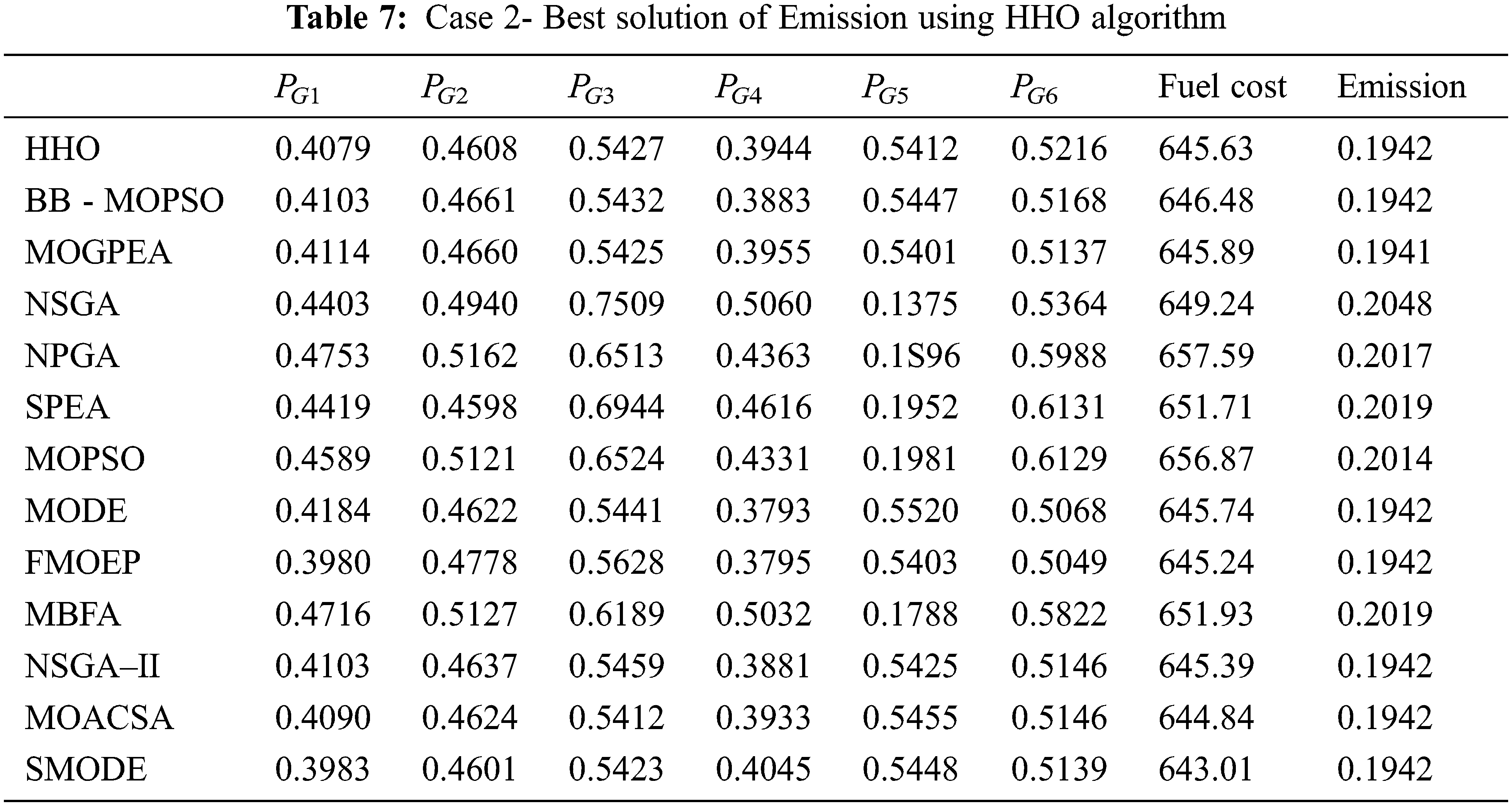
9.2 Evaluation of Solution Quality

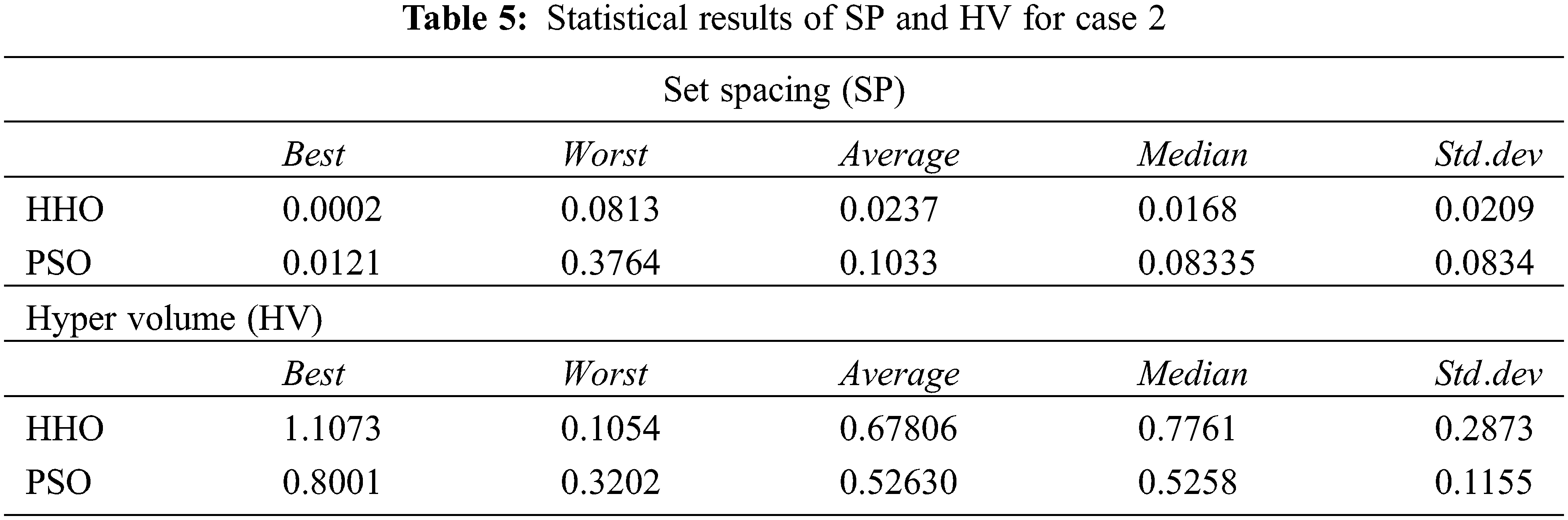
Judging multi-objective performance is a tedious task than single objective method. For evaluating the operation of MOEED approach, it is necessary for computing the eminence of attained non-dominated solution in Pareto front. The solution qualities are compared with the well-known algorithm Multi-Objective Mutated Particle Swarm Optimization (MOMPSO). The commonly used quality metrics are Set Spacing (SP) and Hyper Volume (HV) [22]. Tab. 5 gives the comparison of performance measures of SP and HV. The comparison is made by compiling algorithm for 30 runs.

MOMPSO: inertia coefficient ωmax=0.9, ωmin=0.4, acceleration coefficients = 2

9.2.1 Set Spacing (SP)

The set spacing aids in measuring the similarity of the attained PO set [23]. The formula for this measure is

fspacing=SP2=  1|Ⱥ​​​​|−1∑i=1|Ⱥ​​​​|(d¯−di)2

di=minA/j,A/k∈A/;A/j≠A/k ∑i=1k⁡|fi(A/j)−fi(A/k)| (15)

where di denotes the Euclidian distance of ith non dominated solution with the consecutive solution in Pareto set, d¯ is the mean of all obtained di|A/| . |A| is the pareto set size, A/j,A/k are the solutions in the set. The value zero represent that the values in the set are equally spaced. The non-dominated solutions of HHO algorithm results the minimum spacing (0.0002). It is noted from Tab. 5 that the HHO solutions are better than the solution of PSO, which is significantly represented in Figs. 5 and 6.

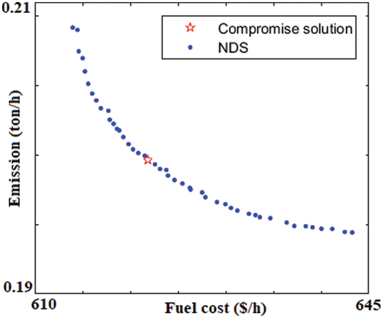
Figure 5: Compromise solution and Pareto front of HHO for case 2

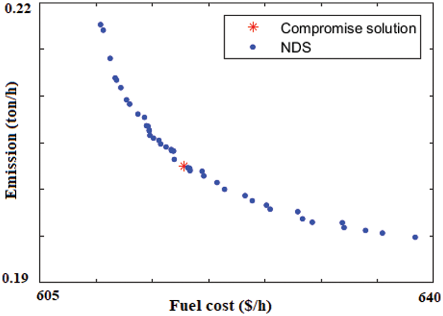
Figure 6: Compromise solution and Pareto front of PSO for case 2

9.2.2 Hyper Volume (HV)

Hyper volume indicator defines the objective function space occupied by the set of non-dominated solution and the reference point pos⊂ℜ . In other words, the union of all hypercubes vi defined by the ith solutions in the PO set and the reference point gives HV

HV=Ui=1|Ⱥ​​​​/|vi={Ua∈Ⱥ​​​​x  :a⪯x⪯xmax}

Here the reference point is considered as the worst value of the objective functions. Since it is the minimization optimization problem, the maximum value of the objective function is considered as reference point. The solutions which poses maximum hyper volume treat as superior. From Tab. 5 the HHO takes the superior place by holding the higher value (1.1073) than PSO

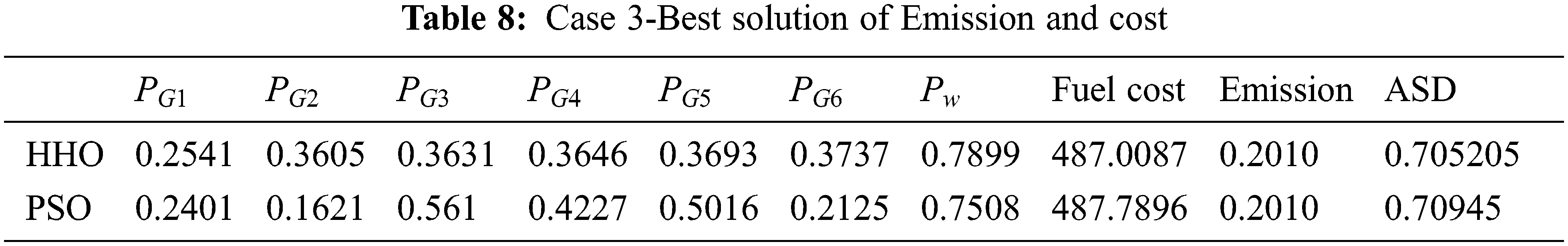
Case 3: In this case the compromising solution and the performance metrics are compared and analyzed for the system with losses and wind generator. Here the 6 thermal generators are accommodated with one wind generator, cut-out wind speed v_o is 25m/s , the rated power of 1.5MW , rated wind speed vr is 15m/s and cut-in wind speed vin is 3m/s . The direct cost coefficient kd,wj is 30$/MWh , the reserve cost coefficient kr,wj and penalty cost coefficients kp,wj are 4 and 2.2 $/MW h. The time series data are download from the National Laboratory Research Centre in hourly resolution. The generated Weibull parameters are calculated as c is 7.2 and k is 5.6, based on modified maximum likelihood method [24].

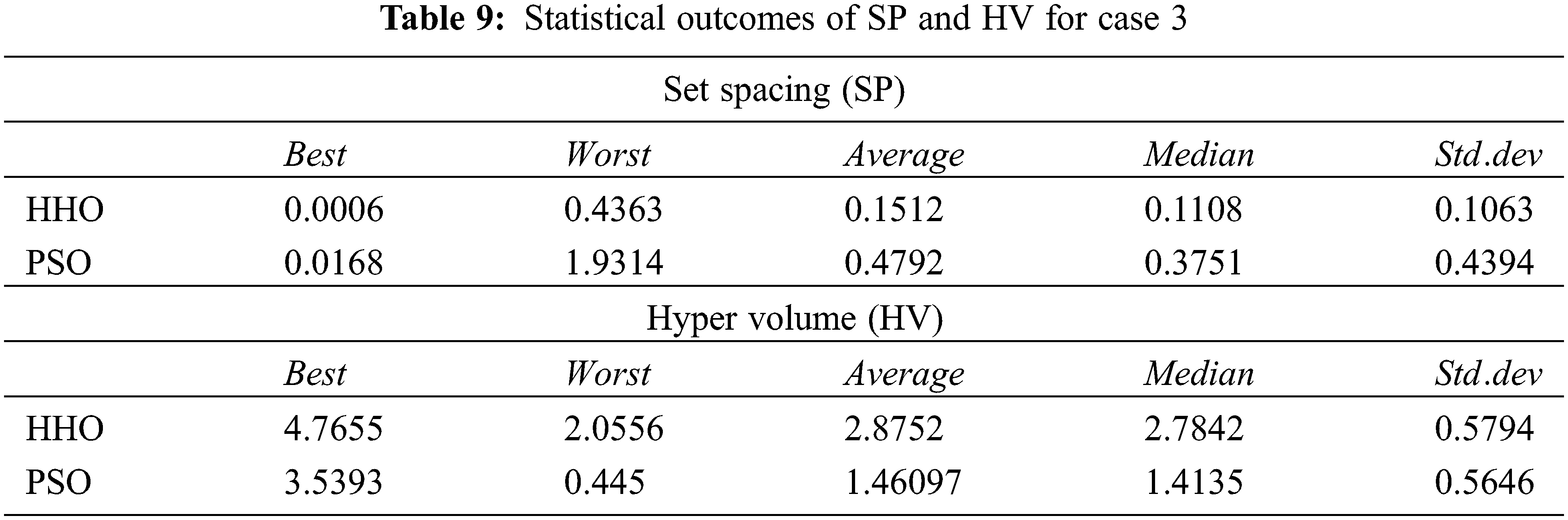
The scheduling of demand among the thermal generator and the wind generator is shown in Tab. 8. According to this the HHO algorithm gives the less fuel cost when compared to PSO. The higher ASD value (0.75205) of HHO prove its efficiency in solving the MOEED problem. The statistical results for case3 are depicted in Tab. 9.

10  Conclusion

The present study has employed a novel long term memory based HHO technique for significantly optimizing the MOEED problem. With the assistance of Clustering technique, the size of PO set is maintained along with the well distributed solutions whereas the compromising solution is extracted from the non-dominated solutions through the implementation of Fuzzy based method. The entire work is validated through IEEE 30 bus 6 generator system and the attained outcomes prove that the HHO produces the optimum outputs than the other optimization approaches. The coding is developed in MATLAB and run-in Intel core i5 processor 2.5 GHz/8GB-RAM system. Moreover, the quality of the non-dominated solutions is examined and analogized with the PSO approach. Therefore, it is validated that the introduced methodology produces optimum solution in solving the MOEED problems.

Funding Statement: The authors have received no specific funding for this study.

Conflicts of Interest: The authors declare that they have no conflicts of interest regarding the present study.

References

 1.  G. Abbas, J. Gu, U. Farooq, A. Raza, M. U. Asad et al., “Solution of an economic dispatch problem through particle swarm optimization: A detailed survey–Part II,” IEEE Access, vol. 5, pp. 24426–24445, 2017. [Google Scholar]

 2.  B. Dey, B. Bhattacharyya and F. G. P. Márquez, “A hybrid optimization-based approach to solve environment constrained economic dispatch problem on microgrid system,” Journal of Cleaner Production, vol. 307, pp. 127196, 2021. [Google Scholar]

 3.  D. W. Ross and S. Kim, “Dynamic economic dispatch of generation,” IEEE Transactions on Power Apparatus and Systems, vol. 99, no. 6, pp. 2060–2068, 1980. [Google Scholar]

 4.  M. R. Gent and J. W. Lamont, “Minimum-emission dispatch,” IEEE Transactions on Power Apparatus and Systems, vol. 6, pp. 2650–2660, 1971. [Google Scholar]

 5.  J. K. Delson, “Controlled emission dispatch,” IEEE Transactions on Power Apparatus and Systems, vol. 5, pp. 1359–1366, 1974. [Google Scholar]

 6.  A. A. Abou El Elaa, M. A. Abidob and S. R. Speaa, “Differential evolution algorithm for emission constrained economic power dispatch problem,” Electric Power Systems Research, vol. 80, pp. 1286–1292, 2010. [Google Scholar]

 7.  G. P. Granelli, M. Montagna and G. L. Pasini, “Emission constrained dynamic dispatch,” Electric Power Systems Research, vol. 24, pp. 55–64, 1992. [Google Scholar]

 8.  U. Guvença, Y. Sonmezb, S. Dumanc and N. Yorukerend, “Combined economic and emission dispatch solution using gravitational search algorithm,” Scientia Iranica D, vol. 19, no. 6, pp. 1754–1762, 2012. [Google Scholar]

 9.  C. R. E. S. Rex, M. Marsaline Beno and J. Annrose, “A solution for combined economic and emission dispatch problem using hybrid optimization techniques,” Journal of Electrical Engineering & Technology, 2019. DOI 10.1007/s42835-019-00192-z [Google Scholar]

10. M. A. Abido, “A niched pareto genetic algorithm for multiobjective environmental/economic dispatch,” Electrical Power and Energy Systems, vol. 25, pp. 97–105, 2003. [Google Scholar]

11. M. A. Abido, “A novel multiobjective evolutionary algorithm for environmental/economic power dispatch,” Electric Power Systems Research, vol. 65, pp. 71–81, 2003. [Google Scholar]

12. M. Basu, “Dynamic economic emission dispatch using non dominated sorting genetic algorithm-II,” Electrical Power and Energy Systems, vol. 30, pp. 140–149, 2008. [Google Scholar]

13. M. A. Abido, “Multiobjective evolutionary algorithms for electric power dispatch problem,” IEEE Transactions on Evolutionary Computation, vol. 10, no. 3, pp. 47–82, 2006. [Google Scholar]

14. Z. Hu, Z. Li, C. Dai, X. Xu, Z. Xiong et al., “Multiobjective grey prediction evolution algorithm for environmental/economic dispatch problem,” IEEE Access, vol. 8, pp. 84162–84176, 2020. [Google Scholar]

15. I. G. Damousis, M. C. Alexiadis, J. B. Theocharis and P. S. Dokopoulos, “A fuzzy model forwind speed prediction and power generation in wind parks using spatial correlation,” IEEE Transactions on Energy Conversion, vol. 19, no. 2, pp. 352–361, 2004. [Google Scholar]

16. S. Li, D. C. Wunsch, E. A. O’Hair and M. G. Giesselmann, “Using neural networks to estimate wind turbine power generation,” IEEE Transactions on Energy Conversion, vol. 16, no. 3, pp. 276–282, 2001. [Google Scholar]

17. B. G. Brown, R. W. Katz and A. H. Murphy, “Time series model to simulate and forecast wind speed and wind power,” Journal of Climate and Applied Metrology, vol. 23, no. 8, pp. 1184–1195, 1984. [Google Scholar]

18. J. Hetzer, D. C. Yu and K. Bhattarai, “An economic dispatch model incorporating wind power,” IEEE Transactions on Energy Conversion, vol. 23, no. 2, pp. 603–611, 2008. [Google Scholar]

19. S. Roy, “Market constrained optimal planning for wind energy conversion systems over multiple installation sites,” IEEE Transactions on Energy Conversion, vol. 17, no. 1, pp. 124–129, 2002. [Google Scholar]

20. Y. Liu and N. K. C. Nair, “A Two-stage stochastic dynamic economic dispatch model considering wind uncertainty,” IEEE Transactions on Sustainable Energy, vol. 7, no. 2, pp. 819–829, 2015. [Google Scholar]

21. S. Mirjalili, H. Faris, I. Aljarah, M. Mafarja and H. Chen, “Harris hawks optimization: Algorithm and applications,” Future Generation Computer Systems, vol. 97, pp. 849–872, 2019. [Google Scholar]

22. J. R. Schott, “Fault tolerant design using single and multicriteria genetic algorithm optimization,” B.S United States Air Force, pp. 1–201, 1995. [Google Scholar]

23. A. Auger, J. Bader, D. Brockhoff Eckart and E. Zitzler, “Theory of the hypervolume indicator: Ooptimal μ-distributions and the choice of the reference point,” in Proc. of the Tenth ACM SIGEVO Workshop on Foundations of Genetic Algorithms, New York, NY, United States, pp. 87–102, 2009. [Google Scholar]

24. J. V. Seguro and T. W. Lambert, “Modern estimation of the parameters of the weibull wind speed distribution for wind energy analysis,” Journal of Wind Engineering and Industrial Aerodynamics, vol. 85, pp. 75–84, 2000. [Google Scholar]