
 Submit a Paper
 Propose a Special lssue
 Open Access
ARTICLE

Evolutionary Algorithm Based Feature Subset Selection for Students Academic Performance Analysis
1 Department of Computer Science and Engineering, Noorul Islam Centre for Higher Education, Kanyakumari, 629180, India
2 Department of Information Technology, Noorul Islam Centre for Higher Education, Kanyakumari, 629180, India
* Corresponding Author: Ierin Babu. Email:
Intelligent Automation & Soft Computing 2023, 36(3), 3621-3636. https://doi.org/10.32604/iasc.2023.033791
Received 27 June 2022; Accepted 23 November 2022; Issue published 15 March 2023
 View Full Text
 Download PDF
Abstract
Educational Data Mining (EDM) is an emergent discipline that concentrates on the design of self-learning and adaptive approaches. Higher education institutions have started to utilize analytical tools to improve students’ grades and retention. Prediction of students’ performance is a difficult process owing to the massive quantity of educational data. Therefore, Artificial Intelligence (AI) techniques can be used for educational data mining in a big data environment. At the same time, in EDM, the feature selection process becomes necessary in creation of feature subsets. Since the feature selection performance affects the predictive performance of any model, it is important to elaborately investigate the outcome of students’ performance model related to the feature selection techniques. With this motivation, this paper presents a new Metaheuristic Optimization-based Feature Subset Selection with an Optimal Deep Learning model (MOFSS-ODL) for predicting students’ performance. In addition, the proposed model uses an isolation forest-based outlier detection approach to eliminate the existence of outliers. Besides, the Chaotic Monarch Butterfly Optimization Algorithm (CBOA) is used for the selection of highly related features with low complexity and high performance. Then, a sailfish optimizer with stacked sparse autoencoder (SFO-SSAE) approach is utilized for the classification of educational data. The MOFSS-ODL model is tested against a benchmark student’s performance data set from the UCI repository. A wide-ranging simulation analysis portrayed the improved predictive performance of the MOFSS-ODL technique over recent approaches in terms of different measures. Compared to other methods, experimental results prove that the proposed (MOFSS-ODL) classification model does a great job of predicting students’ academic progress, with an accuracy of 96.49%.Keywords
Recently, different kinds of learning management systems (LMSs) have been effectively adopted by higher education institutions and universities, collecting large amounts of educational data and recording various student learning features [1]. Educational Data Mining (EDM) is a rapidly expanding scientific field that provides the potential to analyze these information and harness useful knowledge from it. Eventually, a plethora of prediction algorithms have been efficiently used in an educational context to resolve a great number of challenges [2]. But, creating prediction methods in the field of EDM by using TL models has been poorly studied until now. Thus, the most important question in current research is whether a prediction algorithm trained on a previous course would perform well on a novel one [3]. observes that a course (a) is populated with distinct instructors and students, (b) may have features that could not be transmitted (for example, a feature determined on specific learning resources that is inaccessible on other courses) and (c) would change over time in different ways, despite being structurally and contextually distinct. Additionally, the difficulty in course design and the LMS have a great influence on the course progress at the time of semester. Hence, there might be a problem where the transfer learning (TL) method might not reflect the anticipated result, which shows some uncertainty regarding the prediction accuracy of the recently established learning algorithm [4].
Prediction and students’ performance analysis are the two extensively discussed areas of research in educational systems [5]. Despite their disparate goals, the outcomes of performance analysis have a significant impact on predictive research. The analysis of student progress during their studies offers university management data regarding the possibilities of success for all the students. Conventionally, this analysis can be made by the lecturers who utilize their communication with students in classroom activities and mid-term assessments to take timely action and find those “at risk” of dropping out [6]. In the current scheme of higher education, the communication time between students and lecturers is continuously decreasing and finding endangered students has become even more challenging. This is because of the increasing number of students and access to online learning resources for students [7]. More precise predictions of student’s success could be achieved by the current systems of machine learning and data mining analysis.
The prediction of learner performance can be accomplished with the help of several data mining approaches. For example, the machine learning (ML) methods as stated in research works of [8] 2020. The data mining systems are categorised as (a) ML algorithms (like neural networks, symbolic learning, swarm optimization), (b) statistical approaches (namely cluster analysis, regression analysis, discriminant analysis) and (c) artificial intelligence techniques (for example, fuzzy logic, genetic algorithms, neural computation). In this regard, the present study aims at examining the capacity of artificial neural networks (ANN) to forecast team’s performance. Generally, ANN is a subdivision of Artificial Intelligence (AI), which includes the application of Deep Learning (DL) and Machine Learning (ML). The ANN theory was stimulated by the human brain and especially by the biological neural networks. It contains synapsis node for perceptrons and artificial neurons.
The synopsis is found in neural connections and the biological brain is used for learning and memory. The connection strength, i.e., the synaptic weights corresponding to the memorized data, can be changed at the time of the learning method. An array of neurons composes an ANN layer [9]. Usually, all the neurons receive signals (the weighted amount of their inputs), next process them and employ an activation function for signaling neurons related. A simple ANN framework includes output, input, and hidden layers. In contrast, a Deep Neural Network (DNN) method consists of (a) the output layer, (b) the input layer and (c) more than two hidden layers (Denses). The basic functions for training and activating the DNNs are the loss function (feed-forward loop), the optimizer (back-propagation loop) and the activation function [10].
This paper designs a novel metaheuristic optimization-based feature subset selection with an optimal deep learning model (MOFSS-ODL) to predict students’ performance. The proposed MOFSS-ODL technique uses an isolation forest (IF) based outlier detection approach to eliminate the existence of outliers. Moreover, the Chaotic Monarch Butterfly Optimization Algorithm (CBOA) is applied to choose highly related features with low complexity and high performance. Furthermore, a sailfish optimizer with stacked sparse autoencoder (SFO-SSAE) approach is employed to classify the educational data. To validate the enhanced predictive outcome of the MOFSS-ODL technique, a series of simulations were carried out against a benchmark students’ performance data set from the UCI repository and the results are inspected under several dimensions.
This section offers a comprehensive review of existing students’ performance analysis prediction models. In Akour et al. [11], an effort has been made to examine the efficacy of utilizing the DL method more precisely to forecast students’ achievements, which could assist in forecasting when the student can complete their degree or not. The simulation result shows that the presented method outperforms the current approach in terms of predictive performance. In Harvey et al. [12], a prediction method is examined and developed in this work for analysing a K-12 education data set. The LR, DT and NB methods are among the two classifications used in the development of these prediction methods. The NB method gives the most accurate predictions for high school students’ SAT and Math scores.
Orji et al. [13] carried out prior research on determining methods of improving student engagement in online learning techniques via data-driven intervention. Student engagement in this work can be described by objective information (activity log of a certain UG course in a TELS). Activity logs are unbiased data and a reflection of students’ actual learning behaviour (uncontrolled). In this work, the logs of student learning activities from TELS are mined, which employed UG courses, to explore variances among student’s learning behaviours as they are related to their engagement levels and academic performance (evaluated based on last grade point on a course). Supervised (RF) and unsupervised (Clustering) ML methods are applied in examining the relationships.
Xu et al. [14] designed a new ML technique to predict students’ performance in degree programs, i.e., one capable of addressing these major problems. The presented model consists of 2 key characteristics. Initially, a bilayer framework including a cascade of ensemble predictors and multiple base predictors was proposed to make predictions according to the student’s evolving performance state. Next, a data-driven technique based on probabilistic matrix factorization and latent factor model is presented for discovering the course significance, i.e., significant enough to construct an effective base predictor.
Hamoud et al. [15] present method-based DT models and recommend the best method-based performances. This method makes use of the three created categories (REPTree, J48 Random Tree and the questionary filled out by the student). The study includes sixty questions that cover the subject, such as social activity, health, academic achievement, and relationships and how this affects student efficiency. A total of 161 questionnaires were collected. This approach was developed using the Weka 3.8 tool [16] investigated data logged by a TEL scheme called Digital Electronics Education and Design Suite (DEEDS) using a machine learning technique. The ANN, SVM, LR, NB and DT classifiers are included in the ML method. When entering input data, the DEEDS approach allows students to perform digital design problems with varying levels of complexity. Reshma et al. [17] use a deep ANN on a set of hand-crafted features extracted from the virtual learning environment clickstream data to forecast at-risk students and provide a measure for earlier intervention in this situation. The results show that the provided strategy performs better in categorization.
Waheed et al. [18] developed a comprehensive study of limitations, hardware resources and performance. This study can be implemented by using Collaboratory to accelerate the DL method for CB and another GPU-centric application. The selected test-case is a parallel tree-based combinatorial search and 2 CV applications: object segmentation or localization and object classification or detection. The hardware under the accelerated running time is related to a conventional workstation and strong Linux servers armed with twenty physical cores. Cyril et al. [19] proposed a new end-to-end DL technique and suggested a DPCNN method for predicting students’ performances. This paper also presents multitasking learning methods and forecast the performance of students from different majors in an unified architecture.
In this study, an effective MOFSS-ODL technique was designed to predict students’ performance. The proposed MOFSS-ODL technique encompasses IF-based outlier detection, CBOA-based feature selection, SSAE-based classification, and SFO-based parameter optimization. Fig. 1 illustrates the overall working process of the proposed MOFSS-ODL technique.
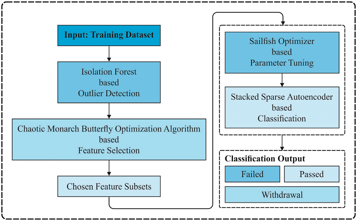
Figure 1: Overall process of MOFSS-ODL technique
3.1 Isolation Forest Based Outlier Detection
At the primary stage, the IF technique is applied to eradicate the presence of outliers in educational data. The IF is an unsupervised algorithm employed in collective-based models to separate the anomalies by evaluating the isolation scores for each data point. The IF has a similar idea of utilising the tree algorithm as the RF model. It processes data points to recurrent random splits that are based on feature selection [20]. The major benefit of the IF technique is how, it processes information. Rather than processing each data point, it employs a DT mode for isolating the outliers, which decreases the processing and execution time and the respective memory requirements. The IF method functions by splitting the algorithm into various segments, which are needed for the subsampling size. The IF estimation starts with specific data points. Next, based on the selected value, it sets a range between the minimum and maximum values to define the outlier scores for all the data points in the tree. The score can be measured by setting a path length for isolating the outliers.
3.2 CBOA Based Feature Selection Technique
During the feature selection process, the CBOA is utilized to choose an optimal subset of features from the educational data; the concept of the BOA method is established in [21]. In BOA, each monarch butterfly is idealized and situated in Mexico (Land 2), southern Canada (Land 1), and the northern US. Next, the position of the monarch butterfly is upgraded in two ways, such as through butterfly adjusting and migration operators. Initially, the offspring are produced (a position upgrade) via the migration operators. Next, the position of another monarch butterfly is upgraded using the butterfly adjusting operators. Furthermore, both operators could be performed concurrently. Thus, the BOA method is appropriate for similar processing and has a good balance of diversification and strengthening. The BOA method includes two significant operators, which are listed below.
In migration operator, the aim is to upgrade the migration of monarch butterflies among Land1 and Land2.
In which
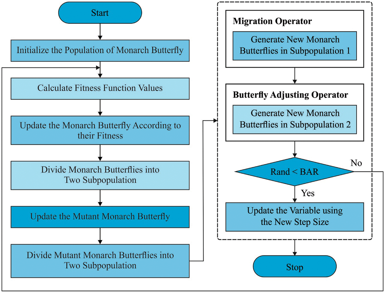
Figure 2: Flowchart of BOA
In the butterfly adjusting operator, it upgrades the location of monarch butterfly in Subpopulation2 as:
Let
The presented CBOA method depends on the incorporation of chaotic maps in the typical BOA. The major phases of the presented model can be given in the following.
a) Invoke the chaotic map to update butterfly locations rather than utilizing arbitrary parameters hence it will enhance the CBOA accuracy. They would be adapted by substituting
whereas
b) Transfer CBOA to binary CBOA: Employing the binary CBOA would characterise the searching space in binary values. Hence, the binary CBOA could adoptively search the feature space for optimal feature integration and is predicted to be very simple when compared to the continuous version. Binary CBOA can be given as follows:
Let s be a transfer function, rand
Different from the standard BOA, wherever the solution was upgraded from the exploring space nearby to a continuing value place, in the CBOA, the searching space was demonstrated as a dimensional Boolean lattice. Besides, the solution was upgraded on the corner of the hypercube. In addition, to solve this issue of selecting or not, a given parameter and binary solution vectors were implemented; one relates to the parameter being chosen for comprising the new dataset, and zero relates to anything else. In binary techniques, one uses the step vector for evaluating the possibility of altering a place. The transmission function significantly influences the balance between exploitation and exploration. During the FS technique, if the size of the feature vector was large, the count of various features combined would inclines, for instance, a huge space for exhaustive research. The presented hybrid technique was utilized to achieve this resolve to explore the feature space vigorously and make the right combination of features. The FS falls into multi-objective issues as it requires satisfying many objectives to receive better solutions that minimize the subset of the FS and, concurrently, maximize the accuracy of the outcome for providing a classifier.
Based on what came before, the fitness function (FF) for finding solutions in this state was made so that the two goals could be met in a balanced way.
3.3 SFO-SSAE Based Classification Model
Finally, the SFO-SSAE based classification model gets executed to determine the proper class labels for the educational data. The building block of deep networks for unsupervised learning features is a single AE [23]. It is another kind of ANN model and is architecturally determined by the output, input and hidden layers that compose a decoder and an encoder. In, the encoder transmits the data matrix to a hidden depiction with a tunable number of neural units, followed by a non-linear activation. The procedure can be expressed by Eq. (8).
In which,
Whereas
Let
Here
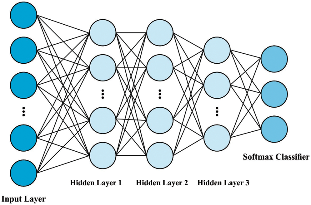
Figure 3: SAE structure
The SFO algorithm is utilized to determine the hyperparameters involved in the SSAE model. The SFO is a new, nature inspired meta heuristic approach, i.e., modelled after a group of hunting sailfish. It displays more competitive performances than widespread meta-heuristic models. The summary of SFO is demonstrated in the following. During the SFO method, the sailfish are considered as candidate solutions and the position of the sailfish in the searching space represents the variable of the problems. The location of
In which
The
Let
Whereas
Now,
Here, B &
In the equation,
While
The benchmark dataset from the UCI repository is used to test the MOFSS-ODL model’s performance. The dataset comprises 649 instances with 33 features and two classes. Table 1 demonstrates the details of dataset decryption. Fig. 4 shows the frequency distribution of the attributes involved in the dataset.
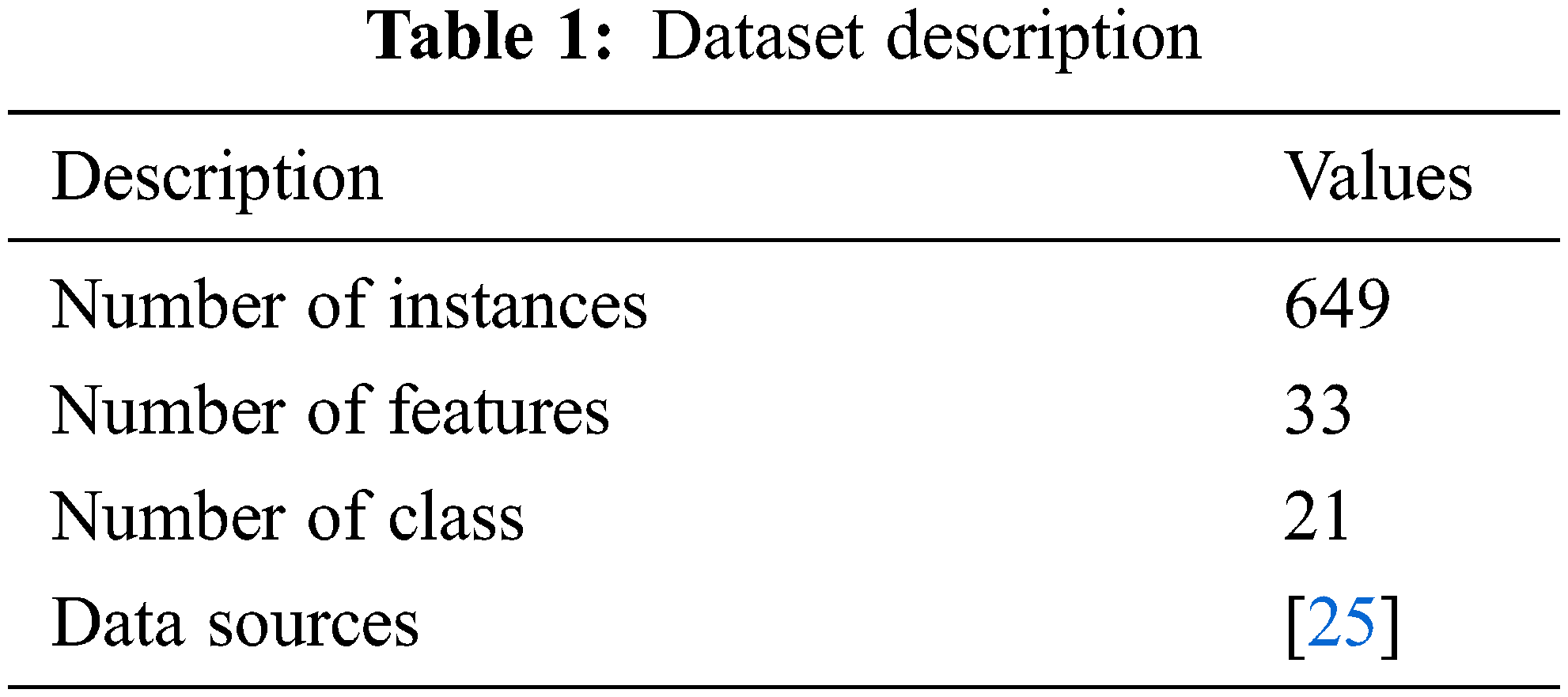
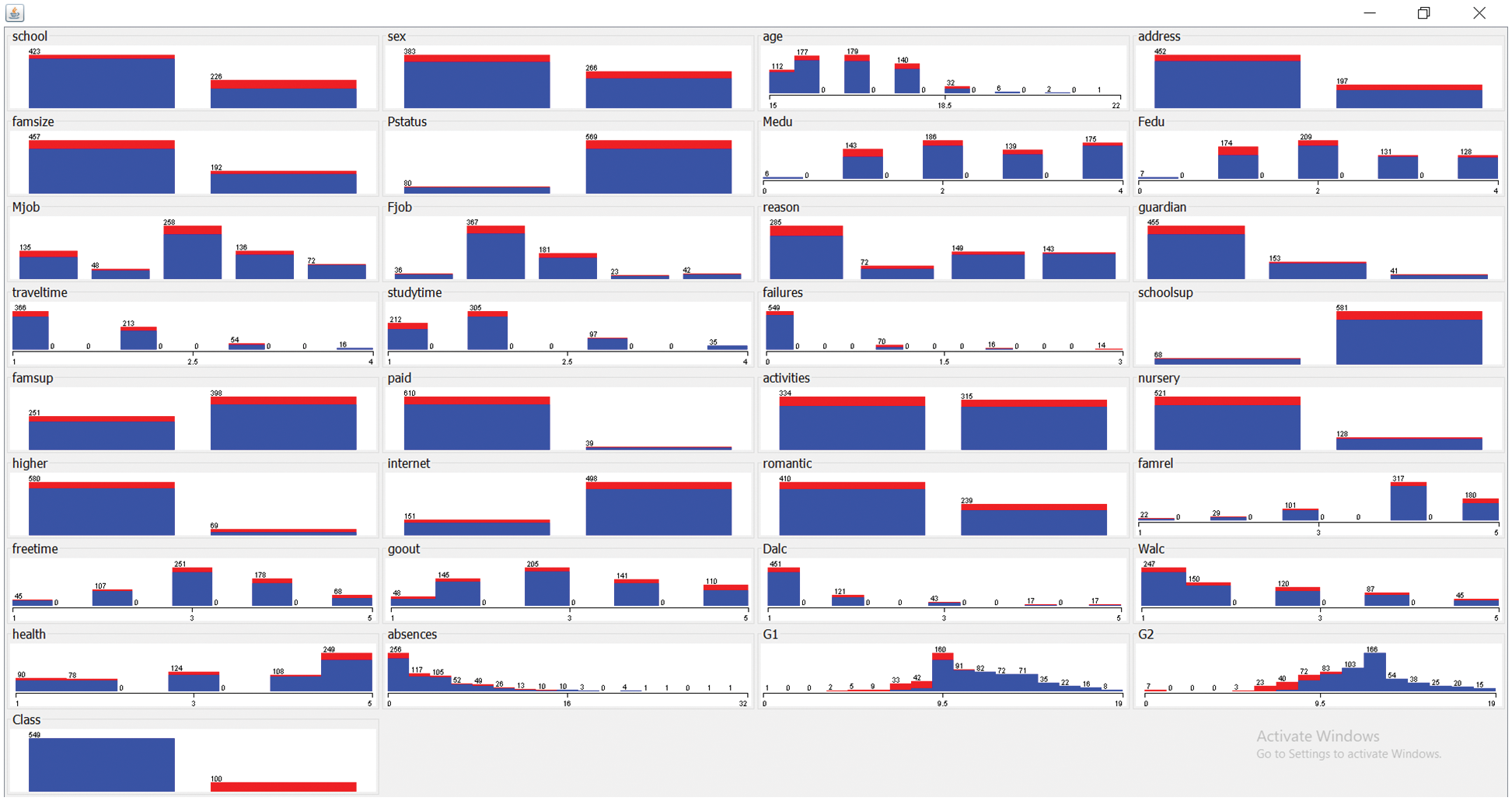
Figure 4: Frequency distribution of attributes in dataset
Fig. 5 Investigate the best cost analysis of the CBOA with other FS models. The results showed that the information gain and CFS techniques have obtained poor performance, with the best costs of 0.38692 and 0.36600. At the same time, the PSO and GA techniques have attained moderate best costs of 0.18364 and 0.16528, respectively. The CBOA method, on the other hand, has led to better performance at the minimum best cost of 0.02411.
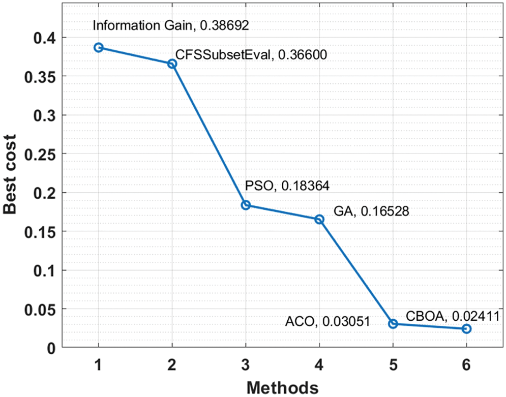
Figure 5: FS analysis of CBOA technique
The confusion matrices generated by the MOFSS-ODL model on the applied dataset under five distinct runs are in Fig. 6. The figures show that the MOFSS-ODL model has classified the instances into two classes effectively. For instance, with run-1, the MOFSS-ODL model has classified 538 instances into class 0 and 87 instances into class 1. At the same time, with run-2, the MOFSS-ODL method has classified 538 instances into class 0 and 86 instances into class 1. Also, with run-3, the MOFSS-ODL approach has classified 540 instances into class 0 and 86 instances into class 1. Concurrently, with run-4, the MOFSS-ODL technique has classified 538 instances into class 0 and 88 instances into class 1. Simultaneously, with run-5, the MOFSS-ODL system has classified 542 instances into class 0 and 88 instances into class 1.
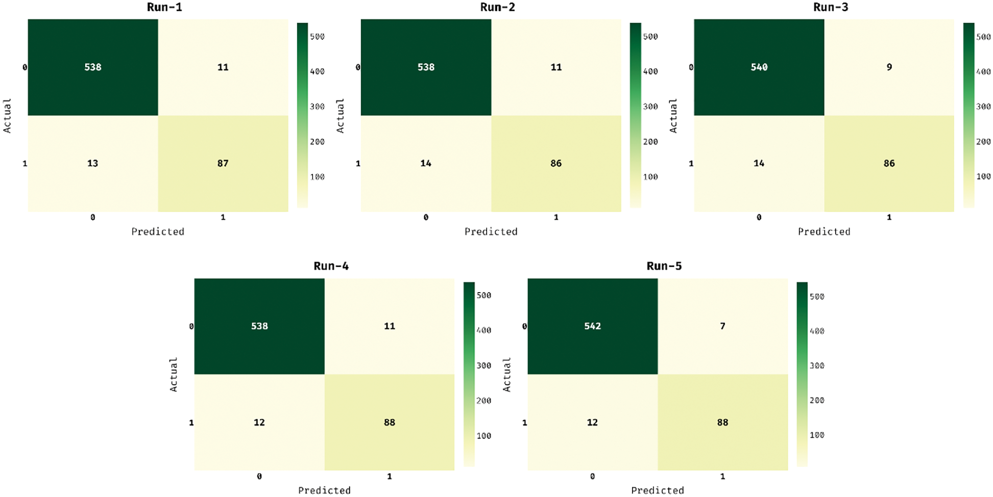
Figure 6: Confusion matrix of MOFSS-ODL model with distinct runs
The values in the confusion matrices are transformed in the form of TP, TN, FP and FN in Table 2.
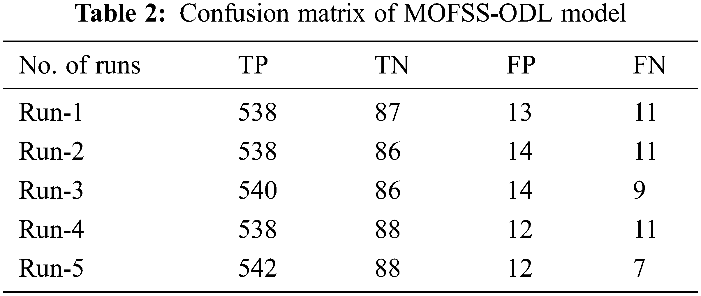
Table 3 offers a detailed classification result analysis of the MOFSS-ODL model under five distinct runs [26–29]. The experimental results reported that the MOFSS-ODL model has accomplished effective classification performance. For instance, with run-1, the MOFSS-ODL model has classified the instances with the
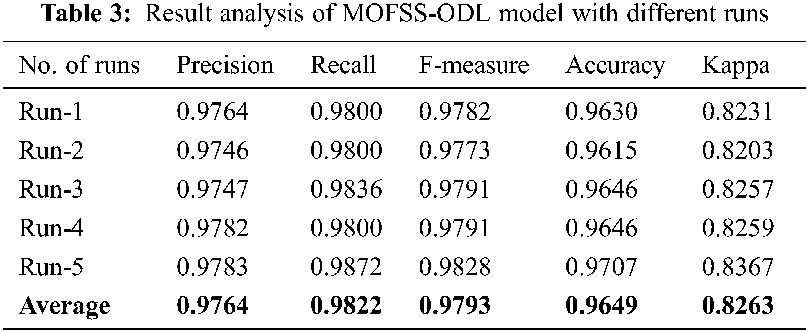
Fig. 7 investigates the average classification outcomes analysis of the MOFSS-ODL model on the test dataset [30–35]. The figure depicted that the MOFSS-ODL methodology has resulted in maximal average

Figure 7: Average analysis of MOFSS-ODL model with different measures
Fig. 8 provides a comparative

Figure 8: Precision and Recall analysis of MOFSS-ODL model
Fig. 9 offers a comparative
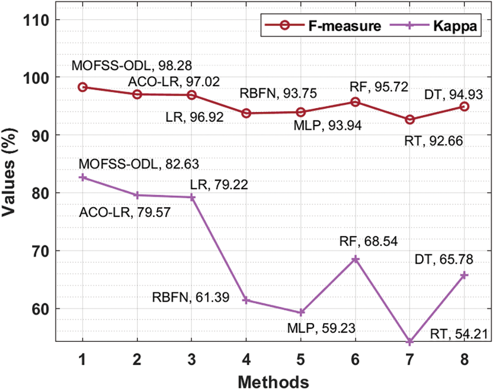
Figure 9: F-measure and Kappa analysis of MOFSS-ODL model
Accuracy analysis of the MOFSS-ODL technique with recent manners takes place in Fig. 10. The figure shows that the RBFN, MLP and RT techniques have obtained lower
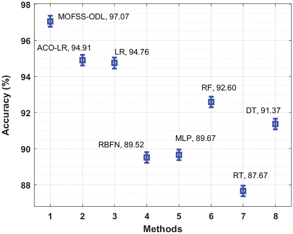
Figure 10: Accuracy analysis of MOFSS-ODL technique with existing approaches
After examining the tables and figures, it can be obvious that the MOFSS-ODL approach has accomplished effective outcomes on students’ performance analysis.
In this study, an effective MOFSS-ODL technique was designed to predict students’ performance. The proposed MOFSS-ODL technique encompasses IF-based outlier detection, CBOA-based feature selection, SSAE-based classification, and SFO-based parameter optimization. Besides, the utilization of CBOA-based feature selection and SFO-based parameter optimization help to accomplish improved students’ performance prediction outcomes. To validate the enhanced predictive outcome of the MOFSS-ODL technique, a series of simulations were implemented, and the outcomes are inspected in several dimensions. The experimental results pointed out the improved performance of the MOFSS-ODL technique over recent approaches in terms of several evaluation measures. In future, the predictive performance of the MOFSS-ODL technique will be enhanced by using the clustering approaches and hybrid algorithms for feature selection on educational datasets to predict students’ achievement.
Funding Statement: The authors received no specific funding for this study.
Conflicts of Interest: The authors declare that they have no conflicts of interest to report regarding the present study.
References
1. R. Asif, A. Merceron, S. A. Ali and N. G. Haider, “Analyzing undergraduate students’ performance using educational data mining,” Computers & Education, vol. 113, no. 1, pp. 177–194, 2018. [Google Scholar]
2. A. Bogarín, R. Cerezo and C. Romero, “Discovering learning processes using inductive miner: A case study with learning management systems (LMSs),” Psicothema, vol. 3, no. 2, pp. 322–329, 2018. [Google Scholar]
3. T. Kavitha, P. P. Mathai and C. Karthikeyan, “Deep learning-based capsule neural network model for breast cancer diagnosis using mammogram images,” Interdisciplinary Sciences: Computational Life Sciences, vol. 14, no. 3, pp. 113–129, 2021. [Google Scholar] [PubMed]
4. C. Romero and S. Ventura, “Educational data mining and learning analytics: An updated survey,” Wiley Interdisciplinary Reviews: Data Mining and Knowledge Discovery, vol. 10, no. 3, pp. 1–10, 2020. [Google Scholar]
5. B. T. Geetha, A. V. R. Mayuri, T. Jackulin, J. L. Aldo Stalin and V. Anitha, “Pigeon inspired optimization with encryption based secure medical image management system,” Computational Intelligence and Neuroscience, vol. 2022, no. 2, pp. 1–13, 2022. [Google Scholar]
6. B. Jaishankar, S. Vishwakarma, A. Pundir, I. Patel and N. Arulkumar, “Blockchain for securing healthcare data using squirrel search optimization algorithm,” Intelligent Automation & Soft Computing, vol. 32, no. 3, pp. 1815–1829, 2022. [Google Scholar]
7. S. Neelakandan, “Large scale optimization to minimize network traffic using MapReduce in big data applications,” in Int. Conf. on Computation of Power, Energy Information and Communication (ICCPEIC), India, pp. 193–199, 2016. [Google Scholar]
8. M. Injadat, A. Moubayed, A. B. Nassif and A. Shami, “Systematic ensemble model selection approach for educational data mining,” Knowledge-Based Systems, vol. 200, no. 1, pp. 1–18, 2020. [Google Scholar]
9. M. Hardas, “Optimization of peak to average power reduction in OFDM,” Journal of Communication Technology and Electronics, vol. 62, no. 2, pp. 1388–1395, 2017. [Google Scholar]
10. R. Farah Sayeed, S. Princey and S. Priyanka, “Deployment of multicloud environment with avoidance of ddos attack and secured data privacy,” International Journal of Applied Engineering Research, vol. 10, no. 9, pp. 8121–8124, 2015. [Google Scholar]
11. M. Akour, H. Alsghaier and O. Al Qasem, “The effectiveness of using deep learning algorithms in predicting students’ achievements,” Indonesian Journal of Electrical Engineering and Computer Science, vol. 19, no. 1, pp. 387–393, 2020. [Google Scholar]
12. J. L. Harvey and S. A. Kumar, “A practical model for educators to predict students’ performance in K-12 education using machine learning,” in 2019 IEEE Symp. Series on Computational Intelligence (SSCI), India, pp. 3004–3011, 2019. [Google Scholar]
13. F. Orji and J. Vassileva, “Using machine learning to explore the relation between student engagement and students’ performance,” in IEEE 2020 24th Int. Conf. Information Visualisation (IV), India, pp. 480–485, 2020. [Google Scholar]
14. J. Xu, K. H. Moon and M. Van Der Schaar, “A machine learning approach for tracking and predicting students’ performance in degree programs,” IEEE Journal of Selected Topics in Signal Processing, vol. 11, no. 5, pp. 742–753, 2017. [Google Scholar]
15. A. Hamoud, A. S. Hashim and W. A. Awadh, “Predicting students’ performance in higher education institutions using decision tree analysis,” International Journal of Interactive Multimedia and Artificial Intelligence, vol. 5, no. 1, pp. 26–31, 2018. [Google Scholar]
16. M. Hussain, W. Zhu, W. Zhang, S. M. R. Abidi and S. Ali, “Using machine learning to predict student difficulties from learning session data,” Artificial Intelligence Review, vol. 52, no. 1, pp. 381–407, 2019. [Google Scholar]
17. G. Reshma, C. Al-Atroshi, V. K. Nassa, B. Geetha and S. Neelakandan, “Deep learning-based skin lesion diagnosis model using dermoscopic images,” Intelligent Automation & Soft Computing, vol. 31, no. 1, pp. 621–634, 2022. [Google Scholar]
18. H. Waheed, S. U. Hassan, N. R. Aljohani, J. Hardman, S. Alelyani et al., “Predicting academic performance of students from VLE big data using deep learning models,” Computers in Human Behavior, vol. 104, no. 2, pp. 1–10, 2022. [Google Scholar]
19. C. P. D. Cyril, J. Rene Beulah, N. Subramani and A. Harshavardhan, “An automated learning model for sentiment analysis and data classification of twitter data using balanced CA-SVM,” Concurrent Engineering, vol. 29, no. 4, pp. 386–395, 2021. [Google Scholar]
20. S. Neelakandan, A. K. Nanda, A. M. Metwally, M. Santhamoorthy and M. S. Gupta, “Metaheuristics with deep transfer learning enabled detection and classification model for industrial waste management,” Chemosphere, vol. 308, no. 20, pp. 1–15, 2022. [Google Scholar]
21. M. Sundaram, S. Satpathy and S. Das, “An efficient technique for cloud storage using secured de-duplication algorithm,” Journal of Intelligent & Fuzzy Systems, vol. 42, no. 2, pp. 2969–2980, 2021. [Google Scholar]
22. P. Ezhumalai and D. Paul Raj, “A deep learning modified neural network (dlmnn) based proficient sentiment analysis technique on twitter data,” Journal of Experimental & Theoretical Artificial Intelligence, vol. 18, no. 2, pp. 1–15, 2022. [Google Scholar]
23. P. V. Rajaram, “Intelligent deep learning based bidirectional long short term memory model for automated reply of e-mail client prototype,” Pattern Recognition Letters, vol. 152, pp. 340–347, 2021. [Google Scholar]
24. S. B. Pokle, “Analysis of ofdm system using dct-pts-slm based approach for multimedia applications,” Cluster Computing, vol. 22, no. 2, pp. 4561–4569, 2019. [Google Scholar]
25. C. Saravanakumar, R. Priscilla, B. Prabha, A. Kavitha and C. Arun, “An efficient on-demand virtual machine migration in cloud using common deployment model,” Computer Systems Science and Engineering, vol. 42, no. 1, pp. 245–256, 2022. [Google Scholar]
26. S. Mishra, P. Mohan, “Digital mammogram inferencing system using intuitionistic fuzzy theory,” Computer Systems Science and Engineering, vol. 41, no. 3, pp. 1099–1115, 2022. [Google Scholar]
27. G. Liu, H. Bao and B. Han, “A stacked autoencoder-based deep neural network for achieving gearbox fault diagnosis,” Mathematical Problems in Engineering, vol. 2018, no. 12, pp. 1–15, 2018. [Google Scholar]
28. P. Santhosh Kumar, B. Sathya Bama, S. Neelakandan, C. Dutta and D. Vijendra Babu, “Green energy aware and cluster-based communication for future load prediction in IoT,” Sustainable Energy Technologies and Assessments, vol. 52, no. 12, pp. 1–12, 2022. [Google Scholar]
29. S. Neelakandan, M. A. Berlin and S. Tripathi, “IoT-based traffic prediction and traffic signal control system for smart city,” Soft Computing, vol. 25, no. 8, pp. 12241–12248, 2021. [Google Scholar]
30. S. Thangakumar and K. Bhagavan, “Ant colony optimization-based feature subset selection with logistic regression classification model for education data mining,” International Journal of Advanced Science and Technology, vol. 29, no. 3, pp. 1–14, 2020. [Google Scholar]
31. V. Ramalakshmi, “Honest auction-based spectrum assignment and exploiting spectrum sensing data falsification attack using stochastic game theory in wireless cognitive radio network,” Wireless Personal Communications-an International Journal, vol. 102, no. 4, pp. 799–816, 2018. [Google Scholar]
32. M. Prakash and C. Saravana Kumar, “An authentication technique for accessing de-duplicated data from private cloud using one time password,” International Journal of Information Security and Privacy, vol. 11, no. 2, pp. 1–10, 2017. [Google Scholar]
33. V. D. Ambeth Kumar, S. Malathi, A. Kumar and K. C. Veluvolu, “Active volume control in smart phones based on user activity and ambient noise,” Sensors, vol. 20, no. 15, pp. 1–13, 2020. [Google Scholar]
34. I. Kaur, V. K. Nassa, T. Kavitha, P. Mohan and S. Velmurugan, “Maximum likelihood-based estimation with quasi oppositional chemical reaction optimization algorithm for speech signal enhancement,” International Journal of Information Technology, vol. 14, no. 6, pp. 3265–3275, 2022. [Google Scholar]
35. S. Satpathy, A. Padthe, V. Goyal and B. K. Bhattacharyya, “Method for measuring supercapacitor’s fundamental inherent parameters using its own self-discharge behavior: A new steps towards sustainable energy,” Sustainable Energy Technologies and Assessments, vol. 53, no. 10, pp. 1–15, 2022. [Google Scholar]
Cite This Article
 Copyright © 2023 The Author(s). Published by Tech Science Press.
This work is licensed under a Creative Commons Attribution 4.0 International License , which permits unrestricted use, distribution, and reproduction in any medium, provided the original work is properly cited.
 Downloads
 Citation Tools