Dual Branch PnP Based Network for Monocular 6D Pose Estimation

1  Introduction

The position and posture estimation of objects are functional tasks of vision systems in robotics. These tasks are widely used in many applications, such as robot vision [1], augmented reality [2] and autonomous driving [3–5]. These tasks are defined by 6D pose estimation, which is used to predict the location of objects in a 3D coordinate system and the orientation of each axis.

From a data perspective, 6D pose estimation approaches can be divided into two categories: depth data-based methods [3,6] and monocular RGB image-based methods [7–9]. Monocular RGB image-based methods are more practical and superior to depth data-based methods in terms of popularity and cost. Therefore, monocular 6D pose estimation has become a research hotspot in the field of computer vision. In addition, from a methods perspective, deep learning-based methods have been successfully applied in many computer vision tasks [10–12]. In recent years, deep learning-based monocular 6D pose estimation methods, such as directly regressing the rotation and translation information [13,14], learning the potential relationship of features [15,16] and using 2D-3D correspondences for 6D pose estimation [17,18], have achieved competitive results. This work focuses on the problem of monocular 6D pose estimation and attempts to find an effective solution to this problem.

Although the performance of monocular 6D pose estimation has greatly improved using 2D-3D correspondence-based methods, these methods still need to be improved in terms of accuracy compared with multiview-based methods [19] and depth data-based methods [3,20]. Through an in-depth understanding of the data information of complex scenes and an analysis of the learning ability of each module in the existing network architecture, it is found that the 3D model points predicted from an RGB image are somewhat different from the actual points. Specifically, due to the information uncertainty caused by occlusion, symmetry and fuzziness of objects, 3D points predicted by deep neural networks have ineradicable errors. In this situation, it is required to capture more effective image features to eliminate the pose estimation errors caused by the failure of 2D-3D correspondence regression. Furthermore, PnP networks, which estimates 6D poses based on 2D-3D correspondences, need to have good learning abilities that can filter unusual features to achieve robust regression.

To solve these problems, in this work, edge map learning and a dual-branch PnP (DB-PnP) network are proposed for 6D pose estimation. First, the edge maps of an object are used to reduce the information uncertainty in a complex scene. The edge maps, which contain rich shape information, are combined with dense correspondence maps that associate plane images and the three-dimensional space, and then these two-layer feature representations can be used to improve the effectiveness and robustness of 6D pose estimation. Additionally, inspired by the multibranch regression of object detection methods, this work proposes separating the rotation and translation regression tasks. Although the transformation matrix is composed of rotation and translation information in the transformation process from the 3D model point to the 2D pixel point, the two variables are essentially different; by transforming the rotation and translation tasks with an allocentric perspective, as in [18], they become independent from each other. Therefore, the same network cannot be applied for the regression processes. Hence, a DB-PnP network is designed to predict rotation and translation information. A comparison between the proposed method and the existing baseline method is shown in Fig. 1. In summary, the contribution of this work can be summarized as follows.

(1)   This paper proposes adding a layer of edge maps to enrich the object shape information, reduce the impact of the correspondence error of 6D pose regression, and improve the accuracy of 6D pose estimation.

(2)   This paper proposes separating the feature learning of rotation and translation matrices and building a two-branch PnP learning network. In the proposed network, the two branches are implemented to simultaneously predict the rotation and translation matrices to highlight the difference between the features of these two tasks, and an attention module is applied to fuse the common features between them.

(3)   The experimental results on the public LM, LM-O and YCB-Video datasets show that the proposed method achieves accurate and robust results for monocular 6D pose estimation. The performance of the proposed method is superior to that of similar methods.

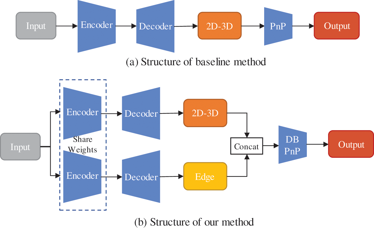
Figure 1: Flowcharts of the proposed method and the existing baseline method

The remainder of this paper is organized as follows. Section 2 introduces the related works, Section 3 describes the algorithms used to implement the proposed method, Section 4 presents and discusses the experimental results, and Section 5 concludes the paper.

2  Related Work

Most monocular 6D pose estimation methods are supervised methods for rigid objects. They can be divided into indirect methods and direct methods. The indirect methods mainly include correspondence-based methods, voting-based methods, and template-based methods. For the direct methods, the transformation matrix is predicted using computational models, especially deep learning-based models. Currently, indirect methods are still the predominant method for monocular 6D pose estimation, especially the correspondence-based method, which has a better prediction effect than the direct method.

The correspondence-based method is a two-stage method that first looks for the 2D-3D correspondences and then uses the RANSAC/PnP algorithm to estimate the 6D pose of objects. In BB8 [21] and YOLO6D [22] the two-dimensional projection of a set of fixed key points, including eight vertices and one center point of a three-dimensional bounding box, are calculated, and the 6D pose of the object is quickly and accurately predicted. When using PVNet [23], the key points are determined by voting. Due to object occlusion, sparse correspondence-based methods are difficult to further improve. To solve this problem, some dense correspondence-based methods, such as CDPN [17] and DPOD [9], have been proposed in recent years.

In references [24,25], a similar idea was adopted to solve the problem of 6D pose estimation. In both of these works, Lie et al. utilized algebra-based vectors and quaternions to represent 6D poses, and a relative transformation between the two poses was estimated for the prediction of the current pose. In [24], the current observation (i.e., the 3D CAD model of the object and the RGB and depth images) and the pose computed in the previous timestamp were applied as input, and the goal was to find a relative transformation from the 6D pose in the previous timestamp to the pose captured by the current observation. In [25], 6D pose estimation was transferred to the problem of iterative 6D pose matching. Given an initial 6D pose estimation of an object in a test image, a relative transformation that matches the rendered view of the object against the observed image is predicted. Different from these works, given an RGB image that contains N objects, the goal of our work is to directly calculate the transformation relationship of each object from the object coordinate system to the camera coordinate system in a real scene. In addition, in [24], the rotation matrix and translation matrix were directly predicted by separate neural network branches composed of convolutional blocks and residual blocks. However, in our work, R and t are predicted by the DB-PnP structure. A convolutional block attention module (CBAM) [26] is applied to improve the performance of the DB-PnP. Although both the method in [24] and the method in our work use two branches to predict the rotation matrix and translation matrix, the ideas and network structures of these two methods are completely different.

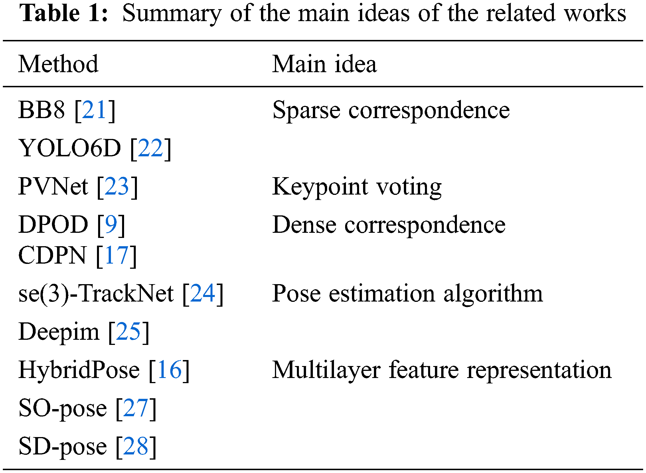
Some researchers have argued that based on the performance of 6D pose regression, it is limited to the use of single correspondence features, but a few multifeature learning methods have been proposed to improve the performance of monocular 6D pose estimation. HybridPose [16] uses mixed intermediate features to represent different geometric information, allowing more diverse features to be utilized for pose regression. Di et al. [27] proposed a self-occlusion pose (SO-Pose) framework to directly estimate the 6D pose from two feature representations, self-occlusion and 2D-3D correspondences. The semantic decomposition pose (SD-Pose) model proposed by Li et al. [28] effectively took advantage of the transferability of the cross-domain 6D pose in different representation domains and integrated different semantic representations to improve performance. Main ideas of these works are summarized in Table 1.

3  Method

In this section, the proposed method is introduced in detail. The overall architecture is shown in Fig. 2. It mainly contains three modules: object image cropping, dense map regression (DMR), and pose estimation. In the first module, the bounding box of the object is obtained from the original RGB image by an object detector. Then, dynamic zoom in (DZI) is applied to the cropped region of interest (RoI), and the RoI of the object is resized to 3×256×256 as the input of the DMR module. The DMR module consists of an encoder, an edge decoder and a correspondence decoder. To predict the edge maps and 3D correspondences, each object RoI is sent to this module. In this process, the mapping of all points on the object should be computed. Therefore, these types of methods are also called dense mapping-based methods. The last module uses the predicted edge maps and 2D-3D correspondences to estimate the rotation and translation matrices.

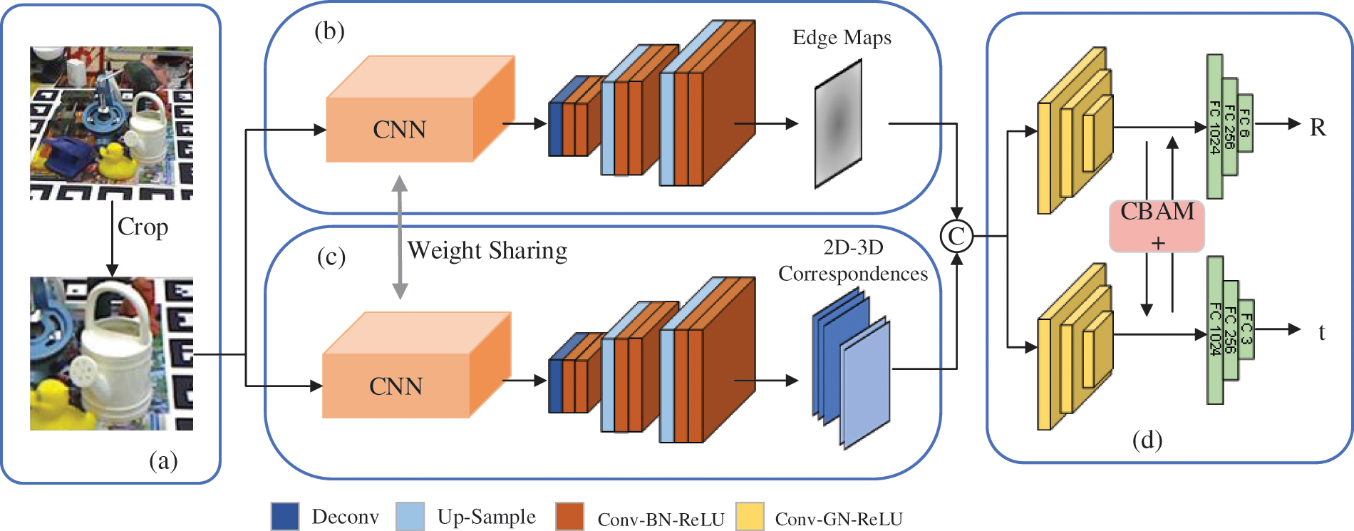
Figure 2: Overall architecture of the proposed method. It contains (a) object image cropping, (b) and (c) dense map regression, and (d) pose estimation

3.1 Dense Mapping Pipeline

Given an RGB image I that contains N objects O = {Oi|i=1,  2, … ,  N} , the goal of 6D pose estimation is to calculate the transformation relationship of each object from the object coordinate system to the camera coordinate system in the real scene, as shown in Fig. 3. R is a 3×3 rotation matrix, and t is a 3×1 translation matrix. Specifically, in this work, R and t are represented by the parameterization method provided in [18,27], which have achieved a much more accurate estimate than the commonly used Lie algebra-based vector. In particular, the origin of the object coordinate system is the center of the object. The 6D pose can be defined as P = {R | t} .

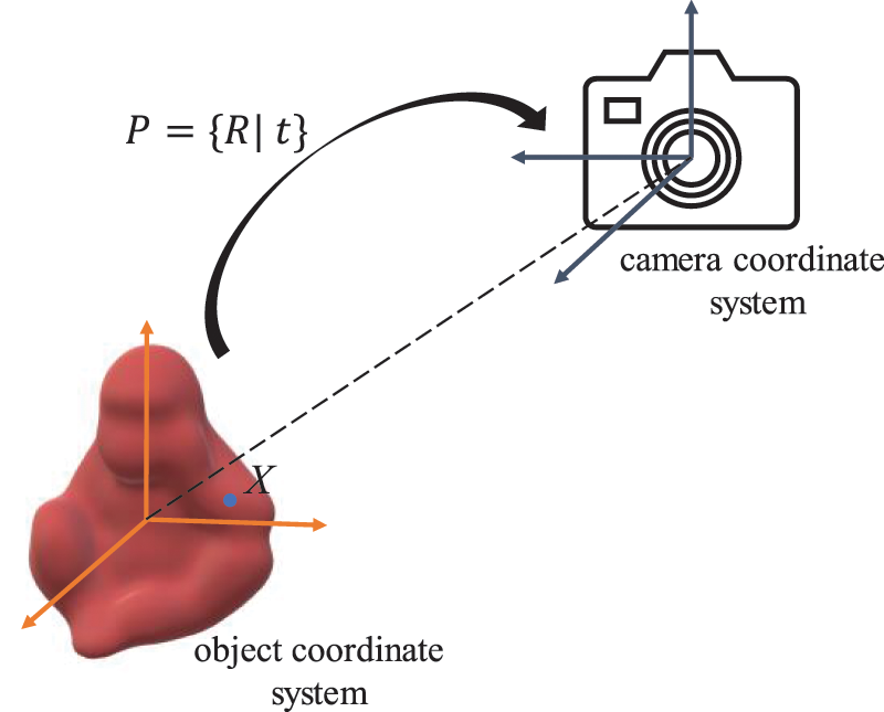
Figure 3: Transformation relationship between the object coordinate system and the camera coordinate system

To obtain the 6D pose, at the beginning of the proposed pipeline, the RoI of each object is fed into convolutional neural networks for feature extraction. In this work, ResNet34 [29] is applied as the feature encoder to make a fair comparison with the baseline method [18], which also used ResNet34 as the feature backbone. This can further highlight the effectiveness of the proposed strategy of 6D estimation. In addition, compared with many deep neural networks without shortcuts, the convergence effect of ResNet with residual blocks will not deteriorate even if the number of network layers increases continuously. ResNet34, excluding the convolutional layer at the beginning and the pooling layer and the full connected layer at the end, has a total of 4 sequence blocks, and each block contains 3 to 6 residual blocks, as shown in Fig. 4.

Figure 4: Overall structure of ResNet34

In the DMR module, there are two branches: edge map regression and 2D-3D correspondence regression. As shown in Fig. 2, these two branches use the same feature extraction network and share the weights. The extracted image feature of the input object is fed into two decoders to predict the edge map and 2D-3D correspondences.

For 2D-3D correspondences, the decoder is designed with the GDR-Net baseline [18], which is composed of a deconvolution layer, an upsampling layer and a convolutional layer. The image feature extracted from the feature backbone is used as the input of the decoder. The decoder consists of one deconvolution layer and two upsampling layers, and both of the deconvolution and upsampling layers are followed by two convolutional units. Each convolutional unit contains one convolutional layer, batch normalization and an ReLU activation function. The output of this decoder is an H×W×C feature map, where H and W are the height and width of the feature map, respectively. C is the number of channels for the 3D maps, surface region attention maps (SRAMs) and mask maps. The 3D maps and 2D maps are spliced together to form 2D-3D correspondences. The 2D maps are tensors of H×W×2 obtained by sampling the u and v coordinate values of the object RoI image. The 2D-3D correspondences and SRAM are used in the following PnP network, and the mask maps are used to remove background information. The loss function of the 2D-3D correspondence regression is defined in Eq. (1).

LCorr=|Mvis¯⊙(MXYZ^−MXYZ¯)|1+|Mvis^−Mvis¯|1+CE(Mvis¯⊙MSRA^, MSRA¯) (1)

where MXYZ , Mvis and MSRA represent the 3D maps, mask maps and SRAM respectively. ∗^ and ∗¯ represent the output and ground truth respectively. And ⊙ represents the multiplication operation. CE(⋅) is the cross entropy function. |∗|1 is the L1 function.

3.2 Edge Enhancement

In complex scenes, due to the occlusion of objects and dim light, there are few visible areas and few textures on objects. The features extracted from a single RGB image are limited, so the predicted 3D model points are bound to have errors, such as offsets or anomalies of 2D-3D correspondences. Complete reliance on unstable correspondences will lead to incorrect 6D pose estimations. Considering this limitation, it is necessary to find more robust and effective features to enhance the input of pose estimation. In dense high-level semantic maps, both surface texture information and spatial information can be used to estimate pose information. Spatial information is difficult to predict without stable structure representation. In this regard, edge maps are adopted as the second representation because they not only contain rich surface texture information but are also easy to obtain.

The network structure of the edge decoder is the same as that of the correspondence decoder. For edge map regression, the image feature extracted from the feature backbone is sent to the edge decoder. The output layer of the decoder is set to H×W×1 , which represents the surface edge of the visible object. H and W are the height and width of the feature map, respectively, and are set in the same way as that of the output of the correspondence decoder. To train the edge map regression network, Canny edge extractor is used to obtain the edge of the object as the label. The loss function of edge map regression is defined in Eq. (2).

LEdge=|Mvis¯⊙(MEdge^−MEdge¯)|1 (2)

where MEdge^ and MEdge¯ denote the predicted edge map and the label, respectively. Mvis¯ is the mask map predicted in the 2D-3D correspondence decoder, and |∗|1 is the L1 function. Some qualitative results of the edge map are shown in Fig. 5.

Figure 5: Illustration of edge prediction results

3.3 Dual-Branch PnP Network

The DB-PnP is an extension of a patch-PnP network. From the results of previous works [18], it can be observed that translation estimation is often very accurate, but rotation estimation is always more difficult. Although both translation and rotation are variables with three degrees of freedom, their properties are different. For a rotation vector, its direction is the same as the rotation axis, and its length is equal to the rotation angle. It is not appropriate to use the same network to simultaneously calculate these two variables. However, most of the previous works have estimated R and t in a module or by using the same network. Therefore, in this work, the structure with two regression branches is proposed to form the DB-PnP network.

Fig. 6 shows the architecture of the DB-PnP network, which contains two inputs and two outputs to compute the 6D pose in parallel. The predicted edge map and the output of the 2D-3D correspondence module are concatenated as the input features fc of these two branches. The outputs of these two branches correspond to rotation matrix R and translation matrix t . The two branches adopt the same structure; that is, they contain three convolutional units and three fully connected layers. Each convolutional unit contains one convolutional layer, group normalization and an ReLU activation function. The feature extraction process is defined in Eq. (3).

fR=CGR3R(fc)ft=CGR3t(fc) (3)

where CGR3R(⋅) represents the operation of three convolutional units in the branch for estimating R . Similarly, CGR3t(⋅) represents the operation for estimating t . fR and ft are the output features of the corresponding branches.

Figure 6: Dual-branch PnP network

As the separate learning of translation and rotation features leads to a significant increase in rotation accuracy and a slight decrease in translation accuracy, this work applies CBAM [26] to merge the features of the two parallel branches, which alleviates the decrease in the translation accuracy due to the separation. The outputs of CGR3 and CBAM are added and then input into the fully connected layer to predict rotation and translation information, respectively. In this work, the numbers of neurons in the first and second fully connected layers are 1024 and 256, respectively. The number of neurons in the last layer is equal to the dimension of the output matrices. The calculation process is defined in Eqs. (4) and (5).

fR′=CBAMR(ft)R=FC3R(fR+fR′) (4)

ft′=CBAMR(fR)R=FC3R(ft+ft′) (5)

where CBAMR(⋅) and FC3R(⋅) represent the CBAM and fully connected layers in the branch of rotation matrix R estimation, respectively. Similarly, CBAMt(⋅) and FC3t(⋅) represent the functions in the estimations branch of translation matrix t .

3.4 Overall Loss Function

The proposed method predicts the two-layer feature representation by inputting an RGB image and then feeding it into a DB-PnP network for pose estimation. All differentiable units can obtain the pose during regression. The overall loss of the model consists of the correspondence loss, edge loss and pose loss.

L=LCorr+LEdge+LPose (6)

where LCorr and LPose are commonly used as the correspondence loss and pose loss, respectively, and are defined in [15].

4  Experimental Results and Discussion

4.1 Implementation Details

The proposed model is implemented on the PyTorch framework and trained on a GeForce RTX 3090 GPU. This work uses a batch size of 80 and a base learning rate of 5e − 4. All objects use the same network for training, without special distinction between symmetric objects and asymmetric objects and without refinement. There are 18493.3 M floating point operations (FLOPs) in the proposed method, and the parameter size is 48.8 M.

4.2 Dataset

Some experiments are performed on the LM [15], LM-O [30] and YCB-Video [8] datasets. The LM dataset consists of 15 videos with a total of 18,273 frames. There are 15 object models in the LM dataset. These models have less texture and slight noise, and each image has only one annotation of an object with almost no occlusion. According to official instructions, 85% of the LM dataset is used as the test set, and the remaining 15% and 15,000 composite images (1,000 rendering images per model) are used as the training set. LM-O consists of 1214 images from the LM dataset, which provide real poses of eight visible objects with more occlusion. Except for a small amount of real data, most of the training data in the LM-O dataset are composed of synthetic data obtained through physically-based rendering (PBR) [31]; hence, it is a more challenging occlusion dataset. YCB-Video is a more recent and challenging dataset that contains real-world scenarios with occlusion, clutter, and symmetric objects. It comprises approximately 130 K real images of 21 objects. In addition to LM-O, this work also uses the PBR training images generated for the BOP Challenge [31].

4.3 Evaluation Metrics

This work employs the two most commonly used metrics to compare the proposed method with other state-of-the-art methods. ADD is used to measure the percentage of the difference between the projection point and the actual point that is less than the threshold and is generally 10%, 5% and 2% of the object diameter (0.1 0.05 and 0.02 d). ADD(S) is used to evaluate symmetric objects. These metrics are defined as follows:

ADD=1m∑x∈M⁡|(Rx+t)−(R^x+t^)| (7)

ADD(S)=1m∑x1∈M⁡minx2∈M|(Rx1+t)−(R^x2+t^)| (8)

where x, x1, x2 are points in the object coordinate system, R and t are the predicted values, and R^ and t^ are the ground truth values. M is the set of points on the object.

In addition, 2∘ and 2 cm are the other commonly used measurement metrics for 6D pose estimation. For rotation matrix estimation, a predicted rotation matrix error of less than 2∘ is regarded as correct. The value of 2∘ measures the percentage of the correctly predicted rotation matrix. Similarly, for translation matrix estimation, a distance between the predicted value and ground truth of less than 2 cm is considered correct. The value of 2 cm measures the percentage of the correct translation rotation matrix. 2∘ , 2 cm represents the percentage of the correct results that meet both conditions.

4.4 Ablation Study

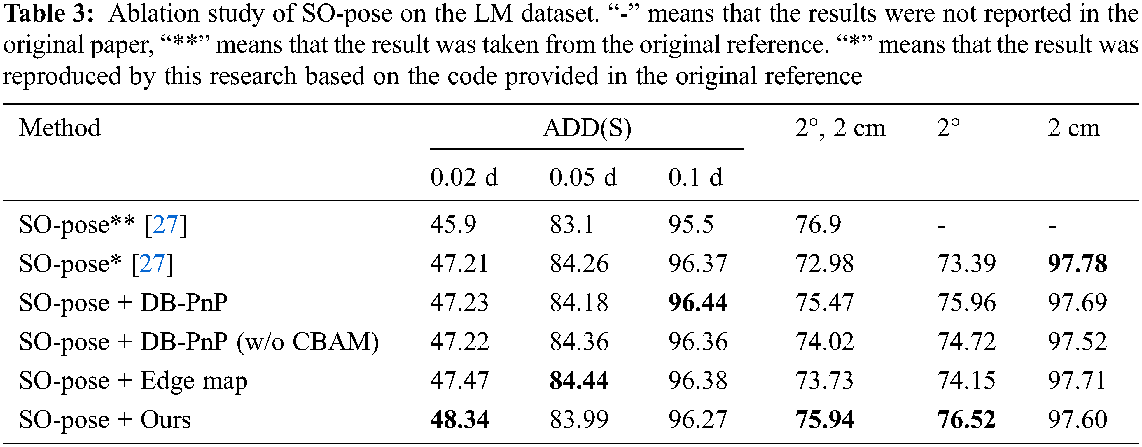
To verify the effectiveness of each component in the proposed method, ablation experiments are performed on the universal LM dataset, with 300 epochs of training for all objects in the related baseline experiments and 360 epochs of training for the validation experiments in [27]. The object detection results provided by [17] are used in the LM dataset. In this experiment, GDR-Net [18] and SO-Pose [27] are applied as the baseline methods.

Tables 2 and 3 show the results of the ablation study. First, due to the equipment difference and some evaluation metric values missing from the baseline methods, the results of the baseline methods are reproduced in Tables 2 and 3. The method in this paper obtains better performance than the original methods, except for the 2∘ , 2 cm metric using SO-Pose. For a fair comparison, this paper implements the proposed method using the same training settings as those used to obtain the reproduced results of the baseline methods and compares the results of the proposed method with the reproduced results to verify the effectiveness of the proposed method.

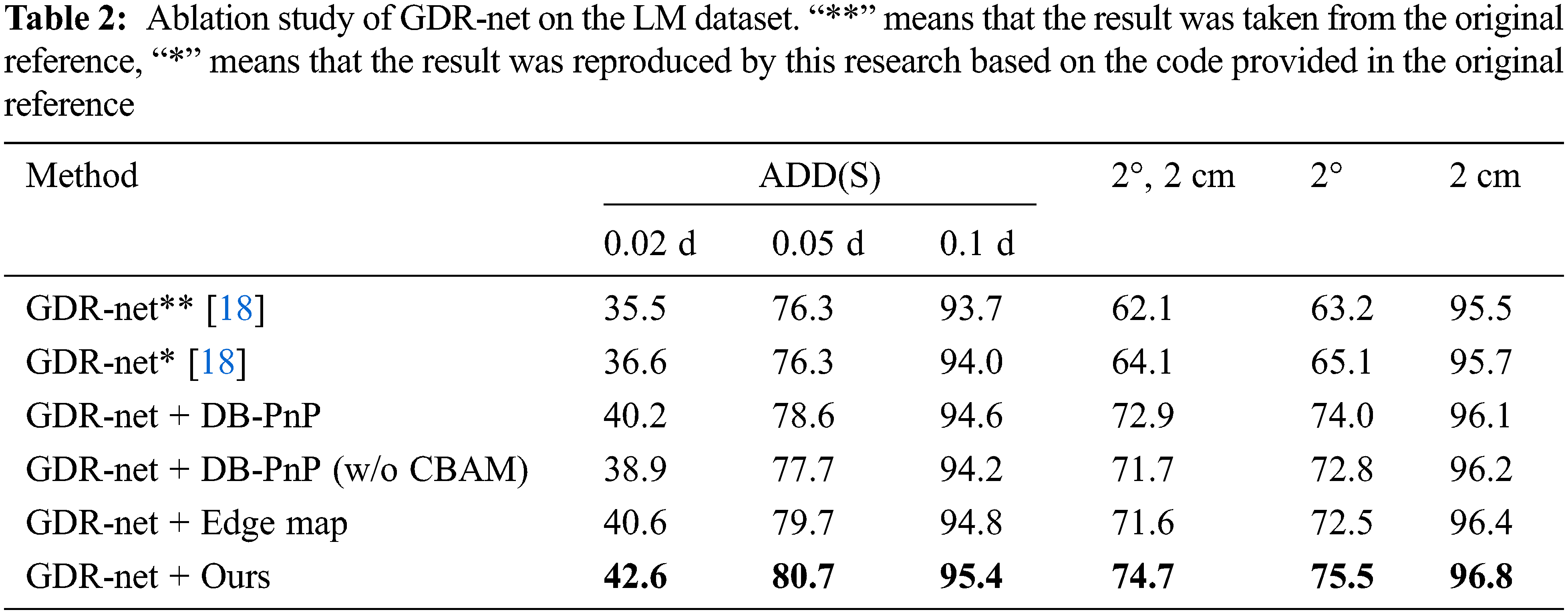
In Table 2, using GDR-Net [18] as the baseline, it can be observed that the results are improved by the addition of the DB-PnP network and the edge map. The DB-PnP network obviously improves the accuracy of rotation estimation, and the edge graph affects the rotation and translation regression results. Compared with the original GDR-Net, by the addition of edge enhancement, the values of ADD(S) are improved from 36.6, 76.3 and 94.0 to 40.6, 79.7 and 94.8, respectively. For the 2∘ , 2 cm metric, the value is improved from 64.1 to 71.6. Compared with the fused DB-PnP and GDR-Net method, the values of ADD(S) can be improved from 40.2, 78.6 and 94.6 to 42.6, 80.7 and 95.4, respectively. For the 2∘ , 2 cm metric, the value is improved from 72.9 to 74.6. All of these results show that the DB-PnP network and edge enhancement are effective in improving the accuracy of 6D pose estimation. The experimental results combined with the DB-PnP network and edge maps show great improvement compared with the baseline results, especially for the 2∘ , 2 cm metric, which increases from 64.1 to 74.7.

To further verify the effectiveness of the proposed method, the proposed edge map and DB-PnP module are applied to the SO-Pose algorithm [27], which adds the self-occlusion feature to the baseline method. The self-occlusion representation proposed by SO-Pose reflects the spatial information of the object, and our edge maps focus on the surface information of the object. Table 3 shows the ablation study on LM. When the DB-PnP network is added to SO-Pose, it has no effect on the 2 cm metric with high accuracy, as it decreases by 0.09, but there is an increase of 2.57 for the 2∘ metric with low accuracy. The 2∘ , 2 cm result is also improved from 72.98 to 75.47. By adding all of our schemes to the SO-Pose model, the rotation accuracy is increased by 3.13. Furthermore, the results of the proposed method using the ADD(S) evaluation metric with the minimum threshold (0.02 d) are increased by 1.1, and it can be observed that the proposed modules are effective under stricter conditions.

Combined with the experimental results in Table 2, it can be observed that when the intermediate representation is not sufficiently accurate and rich, DB-PnP and edge maps can introduce a significant improvement. In addition, from the comparison results in Tables 2 and 3, it can be observed that in DB-PnP, CBAM is effective in improving the results of 6D pose estimation.

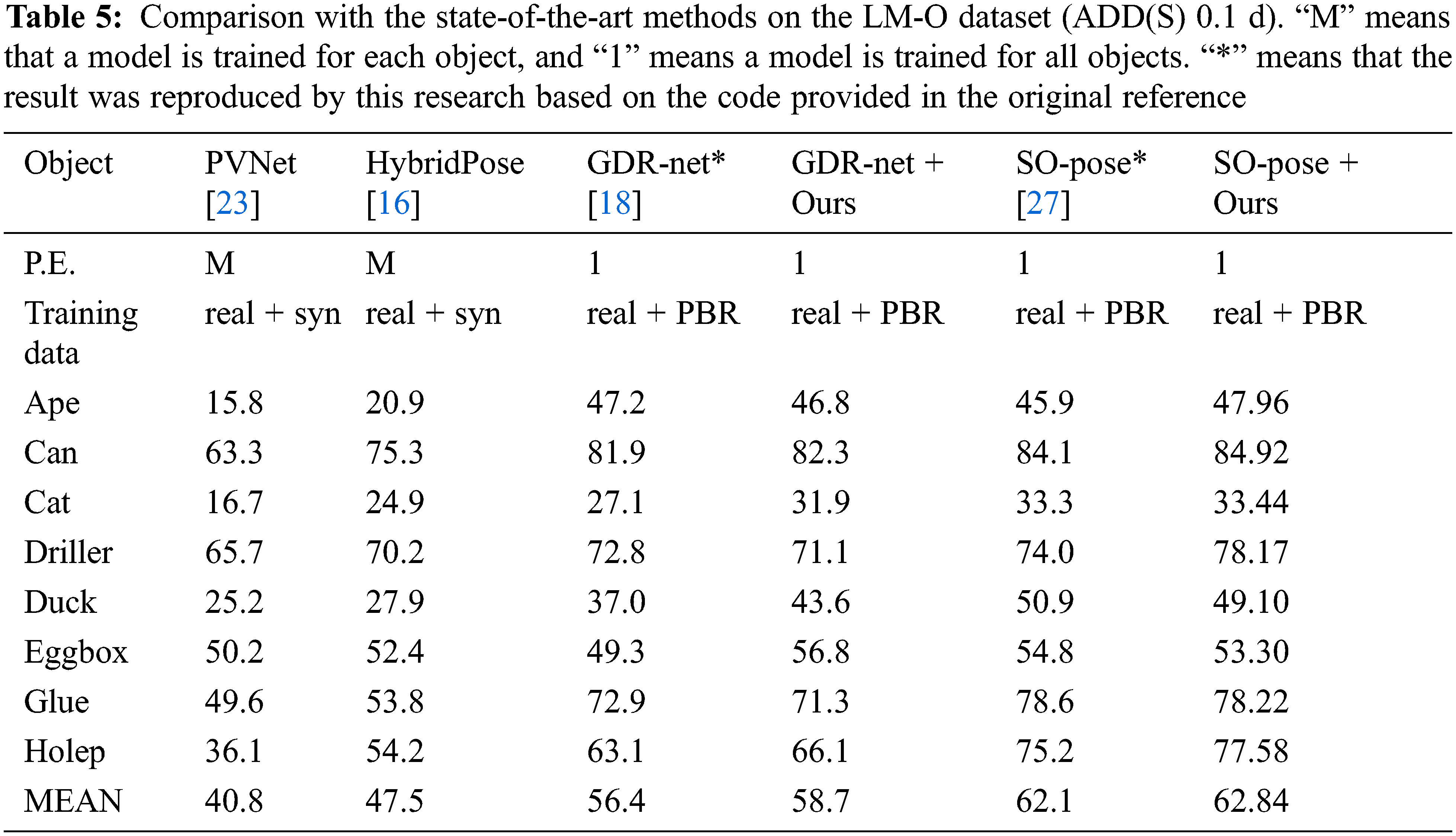
4.5 Comparison with the State-of-the-Art Methods

This paper compares the proposed method with existing methods on the LM and LM-O datasets. In the experiment, for the LM-O dataset, the Faster-RCNN detection results provided by [18] are applied to segment objects from RGB images, and the training data are composed of real data and composite data of PBR. Our method shares one network for all objects. Tables 4 and 5 show the comparison results and reveal that the proposed method is superior to the most advanced methods.

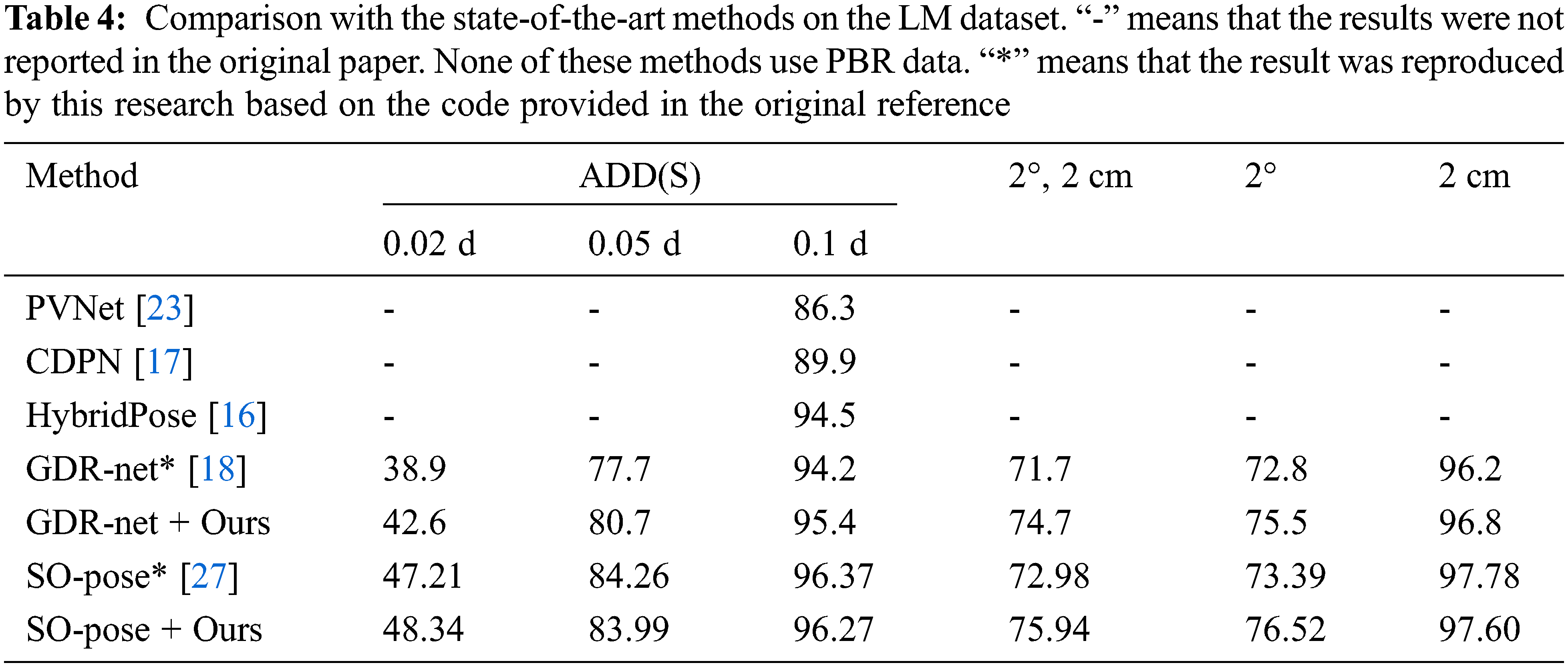
As shown in Table 4, on the LM dataset, the proposed method achieves the best performance in terms of ADD(S) (0.02 d) and 2∘ , 2 cm. metrics. However, from the results in Table 5, on the LM-O dataset, compared with the SO-Pose algorithm, the improvement in the proposed method is not significant. During training, the samples of each batch are randomly selected. Therefore, the model trained each time is slightly different. To ensure the effectiveness of the proposed method, this work repeats the experiment using the SO-Pose algorithm 8 times and reports the mean in Table 5. Compared with SO-Pose, the result is improved from 62.1 to 62.84, and the standard deviation of the proposed method is 0.39. From these experimental results, for SO-Pose, the improvement is not as significant as those for GDR-Net. The main reason is that in SO-Pose, the self-occlusion representation model was proposed to reflect the spial information of the object and improve the intermediate representation. Therefore, the proposed improvement has little impact on the accuracy of the prediction results of SO-Pose.

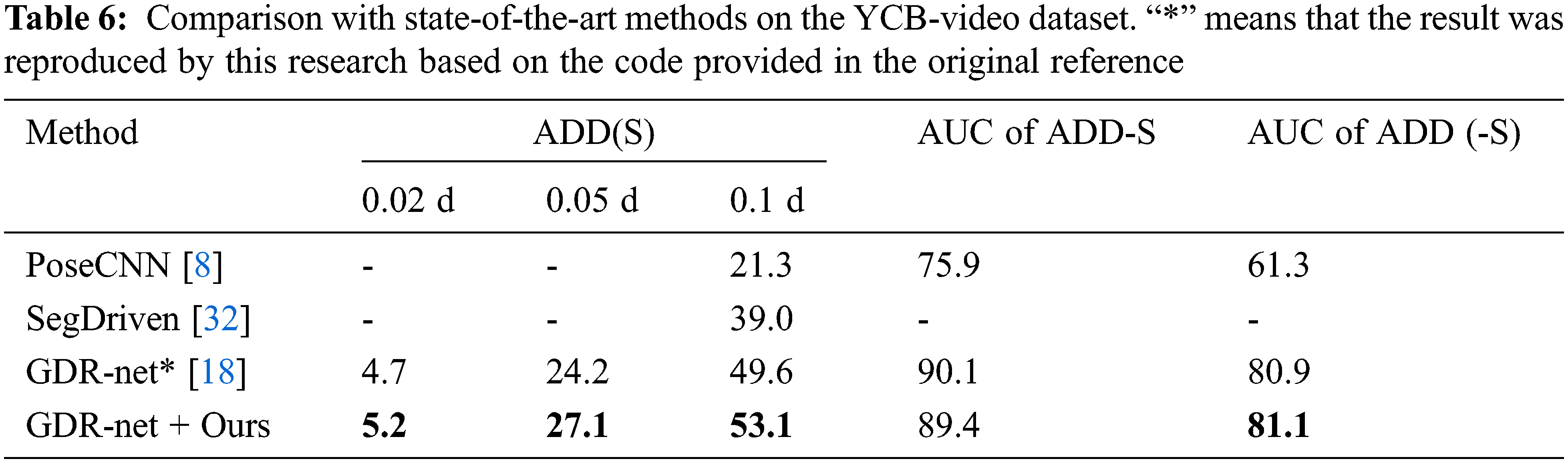
To further verify the effectiveness of the proposed method, the proposed method is applied to the YCB-Video dataset [8]. The experimental results are shown in Table 6. Compared with GDR-Net, the value of ADD(S) is improved from 49.6 to 53.1 after adding the proposed method. From the results on the LM, LM-O and YCB-Video datasets, it can be observed that the proposed method is effective in improving the performance of the baseline methods for 6D pose estimation.

5  Conclusion

In this paper, a two-layer intermediate representation combining edges and correspondence for 6D pose estimation is proposed. Compared with the previous single-layer correspondence representation, the two-layer representation contains richer and more accurate features and uses simple but effective edge features to achieve robust regression. Moreover, the PnP network for estimating rotation and translation information is improved, and the proposed DB-PnP network significantly improves the accuracy of rotation estimation. The results on the public datasets show that the proposed method is superior to the other related works.

The proposed method still has some limitations. The results of ADD(S) (0.1 d) can be further improved on the LM-O and YCB-Video datasets. Furthermore, the proposed method can only estimate instances, and category estimation has not yet been implemented. In the future, the proposed method will be implemented in more complex and challenging scenarios; for example, the estimation of concrete objects will be expanded to the estimation of categories.

Funding Statement: This work was supported by the National Natural Science Foundation of China (No. 61871196 and 62001176), the Natural Science Foundation of Fujian Province of China (No. 2019J01082 and 2020J01085), and the Promotion Program for Young and Middle-aged Teachers in Science and Technology Research of Huaqiao University (ZQN-YX601).

Conflicts of Interest: The authors declare that they have no conflicts of interest to report regarding the present study.

References

1. A. Zeng, K. T. Yu, S. Song, D. Suo, E. Walker et al., “Multi-view self-supervised deep learning for 6D pose estimation in the Amazon picking challenge,” in Proc. ICRA, Singapore, pp. 1386–1383, 2017. [Google Scholar]
2. Y. Su, J. Rambach, N. Minaskan, P. Lesur, A. Pagani et al., “Deep multi-state object pose estimation for augmented reality assembly,” in Proc. ISMAR-Adjunct, Beijing, China, pp. 222–227, 2019. [Google Scholar]
3. C. Wang, D. Xu, Y. Zhu, R. Martín-Martín, C. Lu et al., “DenseFusion: 6D object pose estimation by iterative dense fusion,” in Proc. CVPR, Long Beach, CA, USA, pp. 3338–3347, 2019. [Google Scholar]
4. C. L. Chowdhary, G. T. Reddy and B. D. Parameshachari, Computer Vision and Recognition Systems: Research Innovations and Trends, 1st edition, New York, NY, USA: Apple Academic Press, 2022. [Online]. Available: https://doi.org/10.1201/9781003180593 [Google Scholar] [CrossRef]
5. C. L. Chowdhary, M. Alazab, A. Chaudhary, S. Hakak and T. R. Gadekallu, Computer Vision and Recognition Systems Using Machine and Deep Learning Approaches: Fundamentals, Technologies and Applications, London, England: IET Digital Library, 2021. [Online]. Available: https://digital-library.theiet.org/content/books/pc/pbpc042e. [Google Scholar]
6. M. Tian, L. Pan, M. H. Ang and G. H. Lee, “Robust 6D object pose estimation by learning RGB-D features,” in Proc. ICRA, Paris, France, pp. 6218–6224, 2020. [Google Scholar]
7. W. Kehl, F. Manhardt, F. Tombari, S. Ilic and N. Navab, “SSD-6D: Making RGB-based 3D detection and 6D pose estimation great again,” in Proc. ICCV, Venice, Italy, pp. 1530–1538, 2017. [Google Scholar]
8. Y. Xiang, T. Schmidt, V. Narayanan and D. Fox, “Posecnn: A convolutional neural network for 6D object pose estimation in cluttered scenes,” in Proc. RSS, Pittsburgh, PA, United states, 2018. [Google Scholar]
9. S. Zakharov, I. Shugurov and S. Ilic, “DPOD: 6D pose object detector and refiner,” in Proc. ICCV, Seoul, Korea, pp. 1941–1950, 2019. [Google Scholar]
10. Z. Tian, C. Shen, H. Chen and T. He, “FCOS: Fully convolutional one-stage object detection,” in Proc. ICCV, Seoul, Korea, pp. 9626–9635, 2019. [Google Scholar]
11. Q. Shi, H. B. Zhang, Z. Li, J. X. Du, Q. Lei et al., “Shuffle-invariant network for action recognition in videos,” ACM Transactions on Multimedia Computing, Communications, and Applications, vol. 18, no. 3, pp. 1–18, 2022. [Google Scholar]
12. E. I. Elsedimy, M. Z. Rashad, and M. G. Darwish, “Multi-objective optimization approach for virtual machine placement based on particle swarm optimization in cloud data centers.” Journal of Computational and Theoretical Nanoscience, vol. 14, no. 10, pp. 5145–5150, 2017. [Google Scholar]
13. F. Manhardt, W. Kehl, N. Navab and F. Tombari, “Deep model-based 6D pose refinement in rgb,” in Proc. ECCV, Munich, Germany, pp. 800–815, 2018. [Google Scholar]
14. Y. Hu, P. Fua, W. Wang and M. Salzmann, “Single-stage 6D object pose estimation,” in Proc. CVPR, Seattle, WA, USA, pp. 2927–2936, 2020. [Google Scholar]
15. S. Hinterstoisser, V. Lepetit, S. Ilic, S. Holzer, G. Bradski et al., “Model based training, detection and pose estimation of texture-less 3D objects in heavily cluttered scenes,” in Proc. ACCV, Daejeon, Korea, pp. 548–562, 2012. [Google Scholar]
16. C. Song, J. Song and Q. Huang, “HybridPose: 6D object pose estimation under hybrid representations,” in Proc. CVPR, Seattle, WA, USA, pp. 428–437, 2020. [Google Scholar]
17. Z. Li, G. Wang and X. Ji, “CDPN: Coordinates-based disentangled pose network for real-time RGB-based 6-DoF object pose estimation,” in Proc. ICCV, Seoul, Korea, pp. 7677–7686, 2019. [Google Scholar]
18. G. Wang, F. Manhardt, F. Tombari and X. Ji, “GDR-net: Geometry-guided direct regression network for monocular 6D object pose estimation,” in Proc. CVPR, Nashville, TN, USA, pp. 16606–16616, 2021. [Google Scholar]
19. Y. Labbé, J. Carpentier, M. Aubry and J. Sivic, “Cosypose: Consistent multi-view multi-object 6D pose estimation,” in Proc. ECCV, Glasgow, Scotland, pp. 574–591, 2020. [Google Scholar]
20. Y. He, H. Huang, H. Fan, Q. Chen and J. Sun, “FFB6D: A full flow bidirectional fusion network for 6D pose estimation,” in Proc. CVPR, Nashville, TN, USA, pp. 3002–3012, 2021. [Google Scholar]
21. M. Rad and V. Lepetit, “BB8: A scalable, accurate, robust to partial occlusion method for predicting the 3D poses of challenging objects without using depth,” in Proc. ICCV, Venice, Italy, pp. 3848–3856, 2017. [Google Scholar]
22. B. Tekin, S. N. Sinha and P. Fua, “Real-time seamless single shot 6D object pose prediction,” in Proc. CVPR, Salt Lake City, UT, USA, pp. 292–301, 2018. [Google Scholar]
23. S. Peng, Y. Liu, Q. Huang, X. Zhou and H. Bao, “PVNet: Pixel-wise voting network for 6D of pose estimation,” in Proc. CVPR, Long Beach, CA, USA, pp. 4556–4565, 2019. [Google Scholar]
24. B. Wen, C. Mitash, B. Ren and K. E. Bekris, “Se(3)-TrackNet: Data-driven 6D pose tracking by calibrating image residuals in synthetic domains,” in Proc. IROS, Las Vegas, NV, USA, pp. 10367–10373, 2020. [Google Scholar]
25. Y. Li, G. Wang, X. Ji, Y. Xiang and D. Fox, “Deepim: Deep iterative matching for 6D pose estimation,” in Proc. ECCV, Munich, Germany, pp. 683–698, 2018. [Google Scholar]
26. S. Woo, J. Park, J. Y. Lee and I. S. Kweon, “CBAM: Convolutional block attention module,” in Proc. ECCV, Munich, Germany, pp. 3–19, 2018. [Google Scholar]
27. Y. Di, F. Manhardt, G. Wang, X. Ji, N. Navab et al., “SO-pose: Exploiting self-occlusion for direct 6D pose estimation,” in Proc. ICCV, Montreal, QC, Canada, pp. 12376–12385, 2021. [Google Scholar]
28. Z. Li, Y. Hu, M. Salzmann and X. Ji, “SD-pose: Semantic decomposition for cross-domain 6D object pose estimation,” in Proc. AAAI, Virtual Conference, pp. 2020–2028, 2021. [Google Scholar]
29. K. He, X. Zhang, S. Ren and J. Sun, “Deep residual learning for image recognition,” in Proc. CVPR, Las Vegas, NV, USA, pp. 770–778, 2016. [Google Scholar]
30. E. Brachmann, A. Krull, F. Michel, S. Gumhold, J. Shotton et al., “Learning 6D object pose estimation using 3D object coordinates,” in Proc. ECCV, Zurich, Switzerland, pp. 536–551, 2014. [Google Scholar]
31. T. Hodaň, M. Sundermeyer, B. Drost, Y. Labbé, E. Brachmann et al., “BOP challenge 2020 on 6D object localization,” in Proc. ECCV, Glasgow, UK, pp. 577–594, 2020. [Google Scholar]
32. Y. Hu, J. Hugonot, P. Fua and M. Salzmann, “Segmentation-driven 6D object pose estimation,” in Proc. CVPR, Long Beach, CA, USA, pp. 3380–3389, 2019. [Google Scholar]
Cite This Article
Copyright © 2023 The Author(s). Published by Tech Science Press.
This work is licensed under a Creative Commons Attribution 4.0 International License , which permits unrestricted use, distribution, and reproduction in any medium, provided the original work is properly cited.
Downloads
Citation Tools