Sensor-Based Adaptive Estimation in a Hybrid Environment Employing State Estimator Filters

1  Introduction

Monitoring and managing the position of an object is a major task in navigation.

In recent years, navigation has been conducted using a variety of devices, techniques and methodologies, including compass, coastal navigation, dead reckoning, and charts. The most common types of navigational methods are position fixing and dead reckoning. In order to execute position fixing, one must first determine the navigation states with a predetermined collection of already known places. The use of global navigation satellite systems is an illustration of the positioning technique known as position fixing with Global Navigation Satellite System (GNSS). On the other hand, dead reckoning is a method that determines the navigation states of a moving platform by measuring the progression of such navigation states recursively their initial values. In contrast, live reckoning uses only the initial values of the navigation states.

Despite being the most widely used navigation technology, the Global Positioning System (GPS) suffers from the following limitations: signal degradation due to the environment; signal loss due to barriers; trilateration to determine the exact point of intersection obtained from satellite signals; and signal inaccuracy due to multipath [1]. Although, GPS navigation requires a clear sky to receive precise signals, errors are still possible. As a result, filtering is required for navigation in specific environmental settings so that the environment does not impact GPS receiver signals. GPS receiver signals must be free of interference in order to locate an object’s precise location. Due to disturbance in GPS satellite signal reception, keeping track of these things during surveillance becomes difficult. Continuous reception of noise-free signals is more important for navigation in such applications. [2,3]. Differential Global Positioning System (DGPS) is promoted to overcome the GPS navigation constraint of an object’s erroneous location [4]. DGPS is a part of the GPS that fixes GPS signals positions and eliminates pseudo range errors, which are signal delays and distance differences between a satellite and a GNSS receiver. With this change, GPS receivers can get better information about their location. However, this method is limited because the base station and the user station must look at the same set of satellites. The pseudo range correction has been transformed to World Geodetic System 1984 (WGS84) coordinates and is only applicable when four or more satellites are observed. It is simple to use, but the positioning accuracy will decrease as the distance between the base station and the user station grows [5,6].

A further method combines information from the Global Positioning System with the Inertial Measurement Sensor (INS). However, it has been noticed that the utilization of subject motion limitations was studied to prevent INS error degradation in real-time applications when GPS was unavailable. The main advantage of choosing this approach is that it eliminates the need for an external auxiliary sensor, which helps to keep the system’s cost minimum. The key benefit of taking such an approach is to eliminate the need for an external auxiliary sensor, which helps to keep the cost of the system to a minimum. The INS errors are considerably controlled by the constraints, which improve measurement redundancy, velocity and attitude estimations [7].

Another category for navigation approach is dead reckoning. The need for dead-reckoning navigation arises from the limitations of typical position fixing techniques which require a direct line of sight between the platform, to be navigated, and the well-known fixed positions. With the aid of motion sensors, rotation sensors, state estimator, with inertial navigation system continually calculate the position, orientation, and velocity of a moving object using dead reckoning, without any external references. The inertial measurement unit (IMU) and the processing unit comprise INS [8]. Sensor based navigation will eliminate the need of navigation platform. It is impossible to measure all of a system’s states directly, or some measurements may be unreliable because of measurement errors introduced by the sensors. A real physical quantity the state is detected by a sensor, which then delivers measurement data in the form of an electrical signal output. There are inaccuracies introduced by the converting procedure. Drift error and measurement noise are examples of such inaccuracies. Drift error is eliminated by the sensor’s correction, but measurement noise cannot be eliminated without changing the sensor’s fundamental design.

A state estimation is a method that estimates the internal state of a given actual system, based on measurements of its inputs and outputs. This estimate can predict how the real system will behave in the future. Dynamic state estimation is of tremendous interest to those who investigate state predictors. It allows the system to predict the future by primarily considering the current state of the system as determined by past measurements. Preventative analysis relies on predictive analysis when examining past observations or fixing past mistakes. Data processing is essential to some applications, the data noisy and therefore potentially erroneous. In the case of object tracking, estimation and perdition may lead in the wrong direction due to these incorrect data values [9].This technique of estimating and forecasting is employed in navigation. Typically, regardless of the error covariance, the state estimator should have estimated consistency; if this covariance is inconsistent, it quickly shows system performance issues. A tracking estimator frequently resembles a dynamic state estimator, but with a primary difference of in forecast. This forecast is omitted in state estimation. Without any physical modelling of the system’s time-varying nature, tracking state estimates offer a quick real-time update on its status. Dynamic state estimation simulates the system’s time-altering characteristics, enabling it to anticipate the state vector [10].

A three-axis accelerometer is used for the localization and tracking of a person [11]. The prediction system provides control, preventive and corrective data analysis [12]. This estimation and prediction method is used to process the data from a 3-axis accelerometer and gyroscope, which is then used for navigation without a GPS based on the accelerometer and gyroscope’s raw data. In the Kalman filter, continuous data is monitored with respect to time to provide estimates containing noise and data imperfections. This filter is referred to as the state estimator. The Kalman filter (KF) has a technique based on estimation and prediction implemented for linear time-variant or invariant systems. This filter’s estimation stage is based on measurements that include noise. The prediction phase forecasts the data based on the prior data conditions and current measurement without memory storage, using the previous state as a point of reference. If the values match the expected state, the gain of the Kalman filter will decrease; otherwise, the gain will increase. The Kalman filter is applied since data in a dynamic system is not fixed and is constantly changing. This is the most challenging aspect of the tracking and navigation application. Because of object orientation changes, both the prediction and estimation phases of the Kalman filter become unreliable for navigational purposes [13].

To solve the non-linear estimation problem, the state is linearized using measurement equations, and the resulting linear estimation problem is then solved using the standard Kalman filter formulae. Linearizing a system is as simple as selecting an operational point and approximating the nonlinear function using sensor data. For nonlinear examples of the system beneath each point, the Extended Kalman Filter (EKF) achieves this transformation by linearizing estimates of the mean and covariance of random variables that can be propagated in a nonlinear system. Although it is unstable and appears to have several problems with its convergence capabilities [14], it describes the transformation of mean and covariance estimates. EKF, an extended Kalman filter, is an alternative method for nonlinear Kalman filtering to reduce uncertainty and improve estimation [15].

For the measurement of an estimate, each sensor takes some relative states, and these states of the measurement are biased [16]. These types of estimation can be coordinated with the accelerometer and gyroscope and be fused with the state estimator filters [17,18]. Accelerometer and gyroscope data are fused for state estimation and prediction, regardless of whether the data obtained from them is influenced by noise in linear or nonlinear situation [19,20]. For localization Sigma Point Kalman Filter (SPKF), is applied to nonlinear systems [21]. In this research, the KF, EKF, and SPKF on 3-axis accelerometer and gyroscope data are utilized to determine sensor data patterns under this state estimation model. Table 1 displays a comparison of the three filter variants.

The key contributions of this work are as follows:

•   Sensor data from a 3-axis accelerometer and 3-axis gyroscope are analyzed for localization, estimation, and prediction utilizing a linear and non-linear technique of KF, EKF, and SPKF.

•   Sensor data is the backbone of navigation, and this work will support the sensor data prediction in navigation.

This research paper is divided into sections. Section 2 discusses the fundamental concept of accelerometers and gyroscopes applied to the KF, while Sections 3 and 4 explain the accelerometer and gyroscope testing on the EKF and SPKF, respectively, as well as other considerations for estimating the state of any dynamic system. Section 5 provides an overview of the data set and the experimental setup for data collecting. Section 6 examines the performance of the KF, EKF, and SPKF filters on variant data sets, and Section 7 concludes.

2  Formulation of Dynamic State Estimate Model using Kalman Filter for Accelerometer and Gyroscope

In this section, a dynamic state estimate model based on a Kalman filter is proposed for predicting the activity based on accelerometer and gyroscope estimation. The accelerometer sensor is the primary component that handles acceleration forces with variable velocity. The Kalman filter, is processing a sequence of measurements recorded over time, and while doing so, the environmental and measurement noise affects the data statistics. When an object is in motion, its velocity varies with time. In a precise manner, time is defined in terms of the prior value to calculate the current value, i.e., if suppose the velocity decreases by 3% per time unit, then the current time is 97% of the prior time’s potential.

2.1 Proposed Block Diagram for Accelerometer and Gyroscope Estimation with Kalman Filter

Fig. 1 demonstrates the estimation and prediction of sensor data over time using Kalman filter with accelerometer or gyroscope.

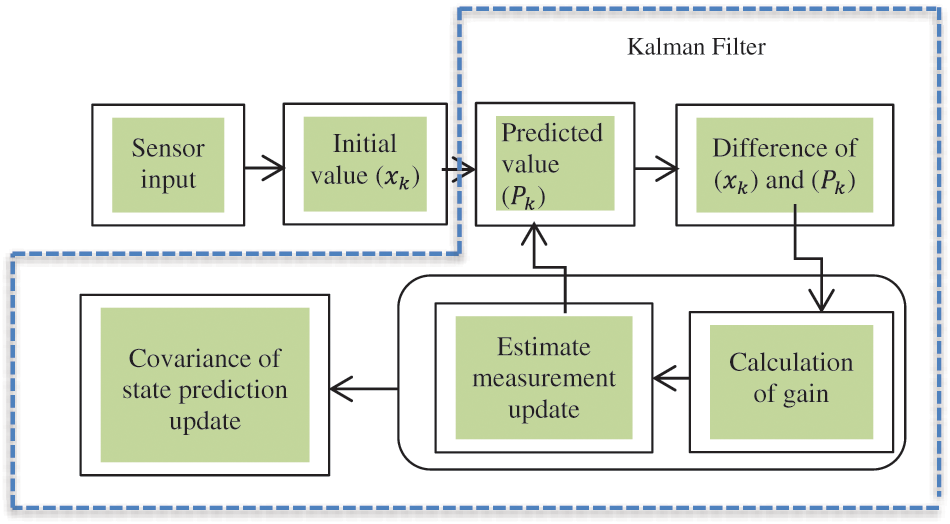
Figure 1: Raw sensor data state estimation and prediction using Kalman filter

Two phases of Kalman filter are estimation and prediction. First stage is the estimating stage, which relies on measurement samples collected in constant time intervals. The nature of the filter is recursive, which means that prediction of the future value is dependent on the present acceleration and location of the sensor. The second stage of Kalman filters is to predict the future values with estimation. This is implemented by taking measurements from sensors and then adjusting an estimate of the state based on both predictions and measured data.

Such measurements are considered as observation values. The following mathematical expressions using the three axes of the accelerometer and constant ‘a’ are used to measure the state of the system.

xk=axk−1+wk(1)

zk=xk+vk(2)

where,

x→Current State of the System,

xk−1→Previous State,

zk→Current Observation,

vk→Noise Measurement,

wk→Process Noise,

a→Constant.

The equations Eqs. (1) and (2) give the Kalman filter state estimate for measuring state x from observations but the noise in the current measurement is unpredictable. Therefore, it is advised to utilize both current and prior measurements and Eq. (1) is re-stated as in Eq. (3).

xk^=axk^+bwk(3)

And the prediction phase is stated using the scaling of the preceding state and can be multiplied by the distribution by a matrix

Pk=apk−1dT(4)

These estimated values are the result of constant state transitions between the previous and present states. To settle the measurement, a relative weight must be added to the current measurement and the previous measurement as given in Eq. (5).

xk^=xk−1^+ck(zk−xk−1^)5)

where,

c=gain.

2.2 Kalman Filter Gain for Estimation

As the gain is added to the estimation, it changes depending on two conditions as given in Eqs. (6) and (7).

Case 1: When the gain is 0, then the estimation is the same as that of the previous estimation and represented as,

xk^=xk−1^(6)

Case 2: When the gain is 1, then the current estimation state is the current observation and represented as,

xk^=zk(7)

For each observation, the estimation of the state is dependent on the current observations, the previous estimate, and gain. In current observation measurements, noise is used to determine the filter’s gain. The accuracy of the accelerometer is dependent on the current measurements, with the gain being calculated based on prediction error and noisy output. With current measurement, previous estimate, and current observation, the state estimate is displayed. So, the gain is represented as in Eq. (8),

ck=ek−1ek−1+m(8)

where,

ek−1→ Prediction error in the previous state

m→ Noisy output from the sensor.

As noise is injected throughout the filter’s prediction stages, the noise variances are permitted to fluctuate with time. This is the covariance of a process estimate and is typically a stochastic variable. It is the average square error prediction. From Eq. (9), the forecast error is calculated as follows:

pk=(1−ck)pk−1(9)

Consequently, if the gain is 1, the prediction error is calculated from the previous value. The first is referred to as a prior estimation, while the second is referred to as an a posteriori estimation [22]. Calculation of time and distance from acceleration must be considered from the acceleration prior to computing the estimation. When velocity is introduced into the system, the current state is calculated as the sum of the preceding velocity and distance at each time step. For several practical equations in the application of accelerometer and gyroscope data for navigation, the Kalman filter has a nearly constant system velocity. As a result, if velocity and distance change over time, the current state of the system can be expressed in terms of the state vector of distance and velocity. Consequently, the prediction and update state equations are denoted from Eqs. (10) to (17).

xk≡[DistanceVelocity](10)

So the prediction and update state equation is represented as,

xk=Axk+Bwk(11)

zk=Cxk+vk(12)

xk^=Axk−1^+Bwk(13)

Pk=Apk−1AT(14)

Gk=PkCT(CPkCT+R)−1(15)

xk^=xk^+Gk(zk−Cxk^)(16)

Pk=(I−GkC)Pk(17)

In Eqs. (11) and (12) A, B and C are matrices for the prediction state and R is taken as the matrix containing covariance between multiple sensor values in the observation zk.

3  Formulation of Dynamic State Estimate Model Using Extended Kalman filter for Accelerometer and Gyroscope

In the non-linear variant of the Kalman filter, a sequence of measurements is recorded over time, and while doing so, noise affects the data statistics. The accelerometer sensor is the primary component that handles acceleration forces with variable velocity. When an object is in motion, its velocity varies with time. Time is precisely specified in a nonlinear state dynamics system; the probability condition density produces the least mean square error with no Gaussian distribution since the output is Gaussian when the Gaussian is fed into a linear system [23]. The Kalman filter always operates with a linear function and numerous sensors whose real-time measurement tends toward non-linearity, resulting in nonlinear sensor readings. As sensor data is not linear and constantly changing, the bulk of sensor values are perturbed, with mean and variance computations being the most affected [24,25] see Fig. 2 below.

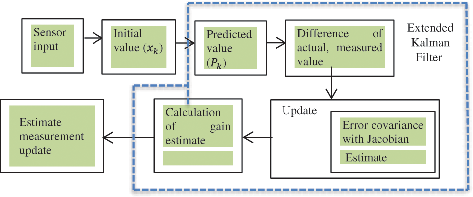
Figure 2: Raw sensor data state estimation and prediction in extended Kalman filter

Kalman filter equation gets modified as the non-linearity is introduced in it. With system dynamics, observations and states are nonlinear. Eqs. (18) and (19) represent the dynamics of a nonlinear system.

xk=xk−1+wk(18)

In an extended Kalman filter, the measurement can also be a nonlinear function of the state and the measurement noise. When the noise is added to the measurement equation, these functions can be written as:

zk=h(xk−1)+vk(19)

The current state and the prediction state in this filter is as of the Kalman filter given in following as:

xk^=xk−1^(20)

pk=pk−1+q(21)

The Kalman gain is the amount of weight given to recent measurements and the current state estimate. If the gain is close to one, the estimated trajectory will be jittery, while a gain close to zero will smooth out noise but make the system less responsive. This gain is represented in the Eq. (22). And the estimated and predicted value is mentioned in the Eqs. (23) and (24).

gk=pkck(pkck+r)−1(22)

xk^=xk^+gk(zk−h(xk)^)(23)

pk=(1−ckgk)pk(24)

In a nonlinear variant of the KF, the prediction state is identical to the Kalman filter’s prediction state except for the update state [26]. The actual signal, sequential difference subtraction, approximation of the signal’s first derivative with time step, and multiple observation space values all influence the update state. Moreover, in cases where the update state is applied, the single-valued nonlinear state is transformed into a multi-valued system with two states and three states in observational space. This matrix referred to as the Jacobian matrix [27,28], contains the current value of the first sensor’s state-value-related first derivative for a nonlinear model.

Due to this state transition model in nonlinear function, the present state estimate and prediction are represented in equations Eqs. (25) to (31).

xk=f(xk−1,uk)+wk(25)

zk=h(xk)+vk(26)

xk^=f(xk−1^,uk)(27)

Pk=Fk−1Pk−1Fk−1T+Qk−1(28)

Gk=PkHkT(HkPkHkT+R)−1(29)

xk^=xk^+Gk(zk−h(xk)^)(30)

Pk=(I−GkHk)Pk(31)

where

f→state transition function

R→Covariance matrix of sensors

P→Process estimation

G→ Gain

H→Jacobian matrix

h→Observation function

Q→Covariance of process noise.

4  Nonlinear Filtering Using Sigma Point Kalman Filter

The Sigma-Point Kalman filter is an alternative method for nonlinear and continuously changing data that uses nonlinear probability distribution functions. This filter functions similarly to the state estimate carried out by EKF in SPKF minus the Jacobian function. In this filter, the estimation approximation of the probability distribution is straight forward than that of any arbitrary nonlinear function [29].

Proposed Block Diagram for Accelerometer and Gyroscope Estimation Using SPKF

The SPKF predicts and updates the stage in a manner comparable to the Kalman filter. The SPKF procedure is depicted in Fig. 3:

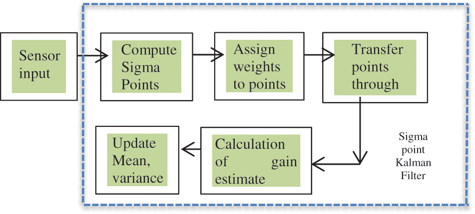
Figure 3: Nonlinear estimation and prediction in sigma point Kalman filter

This filter has three primary steps, with the first step selecting sample points from the input distribution. There may be deterministic values and a certain amount of standard deviation in these random samples [30]. These are known as sigma points, and the corresponding filter is called the sigma point filter. In this algorithm’s second stage, after picking points, the picked sigma points must be processed through a nonlinear function to generate a new output distribution. Moreover finally, these outputs are used to calculate the output’s mean and standard deviation. For an N-dimensional distribution, the sigma points must be chosen as [31],

Sigma points=2N+1(32)

After passing the points through some nonlinear functions, some points from the source Gaussian are mapped to the target Gaussian. It can be very difficult to transform the whole state distribution, but it is easy to transform some individual points of the state distribution as mentioned in the Eqs. (33) and (34).

Now consider the weighted sigma points represented with their approximate mean and covariance,

μ′=∑i=02nω[i]g(x[i])(33)

∑Σ′=∑i=02nω[i](g(x[i])−μ′)(g(x[i])−μ′)T)(34)

where

µ′→Predicted Mean

ω→Sigma points weight

g→Nonlinear function

Σ′→Predicted Covarience

n→Dimention Space.

P=∑i=02nω[I](Z(x[i])−z^)(Z(x[i])−z^)T+Q)(35)

T=∑i=02nω[i](x[i])−μ′)(Z(x[i])−z^)T(36)

K=T.S−1(37)

The data is coming from the sensor and it is essential to map it with the measurement space, denoted by Z. In the prediction phase of the filter, the covariance calculation is done, in which process noise is added. In the update phase, the difference between predicted mean and covariance and actual mean and covariance is evaluated [32]. In the filter gain calculation, there has to be a cross-correlation between the sigma points in state space and the sigma points in measurement space. For the precise operation of this filter, it transforms value from the distribution of a single point’s state distribution via a nonlinear function rather than whole state distribution [33].

5  Methodology

5.1 Dataset Description

The state estimation approach has received data from sensors which has captured the labelled dataset for the indoor and outdoor environment for activities like walking, climbing up a staircase, climbing down a staircase, seating, cycling, and underground basement walk. It uses a pre-processed feature set of 23 features, to evaluate the performance of the localization and tracking. Each record consists of the following attributes: total acceleration, from the three axis of the accelerometer and the estimated body acceleration.

In Fig. 4a, hardware used to capture the data and activities is shown and Figs. 4b and 4c shows the subjects wearing the designed device above the ankle to ensure the position of placing and capturing the various patterns. For training, estimation and navigation patterns I & II, the feature data is gathered from the accelerometer, gyroscope, and GPS. For estimation and prediction, gathered from different environment I (indoor) and environment—II (outdoor), Table 2 shows number of data samples used as training cases for different subjects, captured for duration ranging from 10 to 40 min based on volunteers’ comfort. The trade-off between prediction and estimate is required for systems operating in moving scenarios in indoor and outdoor locations, which are based on dynamic state estimation of the filters as needed in real-time situations and for which prediction accuracy is the ideal goal.

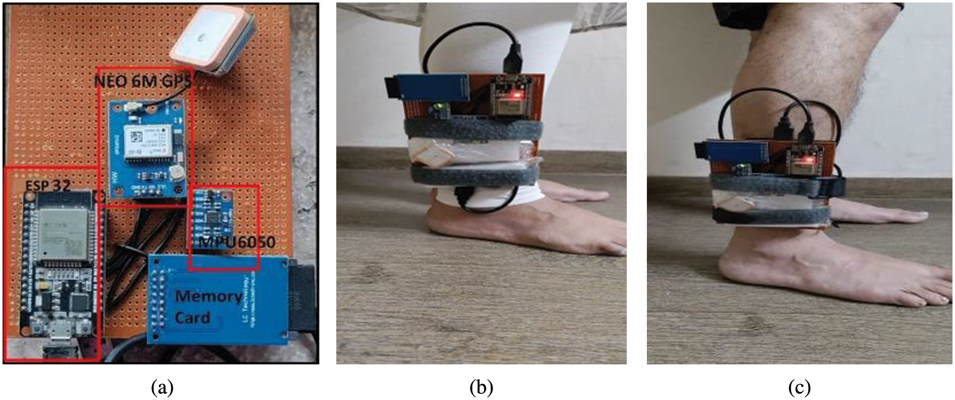
Figure 4: (a) Hardware used to capture data (b) and (c) Different subjects wearing the hardware for generation of indoor/outdoor navigation for labeled activities

5.2 Experimental Conditions for Information Collection

The monitoring of the accelerometer and gyroscope conditions is required either for environment navigation or activity analysis, which requires the reliable assessment of the spectra encountered by the subject, either as a final result or intermediate step for the measurement of the relevant sensor-based-motion parameters. The data collected for the two base classes, indoor and outdoor, for the various activities listed in Table 2 is currently being analysed. For the captured data of indoor and outdoor activity, the exhaustive time-domain analysis and frequency-domain analysis carried are carried out to show that a sensor signal changes over time and the signal’s energy is distributed over a range of frequencies.

Figs. 5a and 5b show the accelerometer and gyroscope raw data for the activity done by the subject for the 3 axis accelerometer and gyroscope. Figs. 6a and 6b show the acceleration plot for the activity using a set of sensor data with different lengths, and environments, followed by Figs. 7a and 7b which show the Welch method and other spectrum estimation methods.

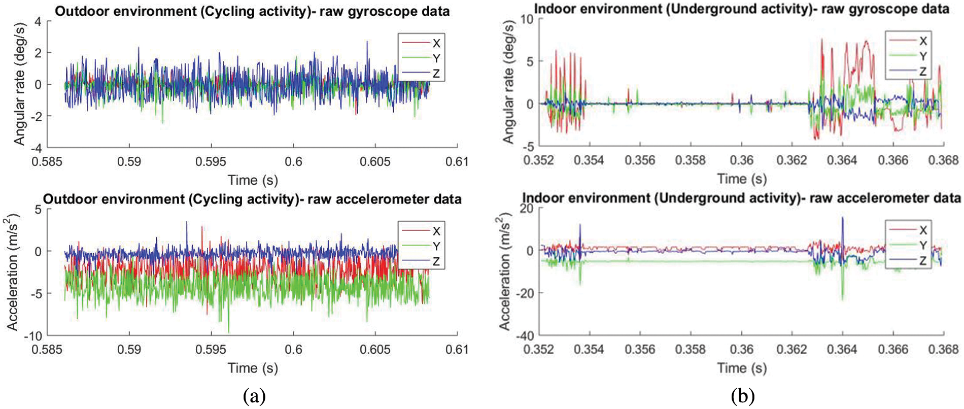
Figure 5: Raw sensor data samples for two classes for different activity environment

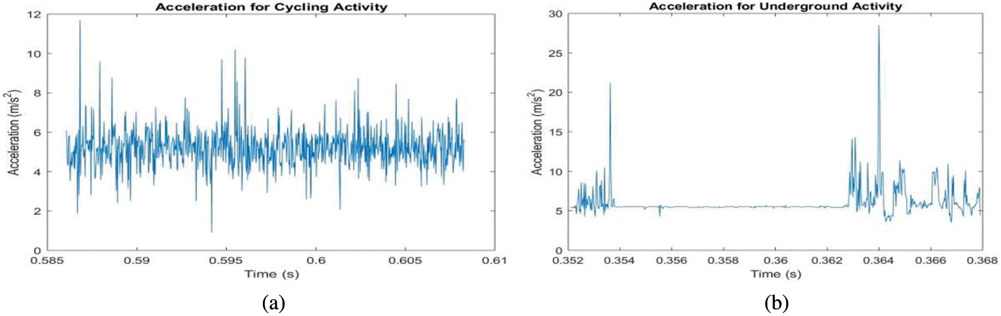
Figure 6: Acceleration for the activity for indoor and outdoor environment

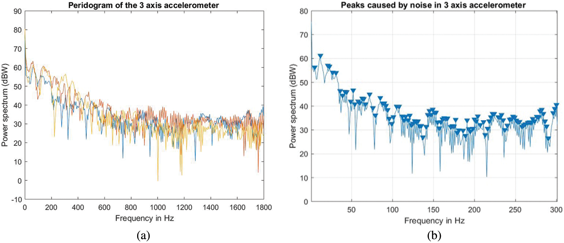
Figure 7: Acceleration for the activity for indoor and outdoor environment

Spectrum reconstruction techniques were used to discover the key sensor state parameters, including significant noise impacts and more accurate power measurements, the mean sensor data value period, and the spectrum peak enhancement factor. Both spectrum analysis and sensor-based state reconstruction methods are explored to provide useful recommendations.

As observed in the preceding graph, the periodogram displays a number of frequency peaks that are unrelated to the signal of interest. Multiple repetitions of the experiment and averaging would eliminate the erroneous spectral peaks and produce more precise power measurements. This is accomplished using the Welch function for averaging.

5.3 Experimental Conditions for Information Collection

The experiments were carried out on a group of ten participants ranging in age from 21 to 40 years. Each subject pursued six activities in a hybrid environment, including walking, climbing upstairs, climbing downstairs, sitting, cycling, and underground walking while wearing an embedded circuit on the subject’s leg, which consists of NEO 6M GPS and MPU6050 sensor with built-in 3-axis accelerometer and gyroscope. The specifications of the sensors used to capture data are mentioned in Table 3. Furthermore, performance of KF, EKF and SPKF need to be taken into consideration for the choice of the best-fitted filter for indoor and outdoor activity for object tracking and localization.

To capture the activities, one prototype module is tied to the ankle of the subject. This significantly improves the capturing of each activity pattern. The experiments are conducted on a sensor-based approach for the subject with different patterns of navigation. Features selected for the database are captured from the raw sensor values of the 3-axis accelerometer and gyroscope for linear acceleration and angular movement.

Performance of state estimator filters carried out by numerical simulation is done using MATLAB 19a tool. The task is tested for the acceleration on the posture for the various environments for different patterns on which the raw accelerometer data is collected by the MPU6050 sensor for state estimation and prediction using the three forms of the Kalman filter, viz., normal KF, EKF and SPKF. The linearity and nonlinearity of the accelerometer and gyroscope are analyzed for three variants of the filter for more accurate state estimation. The first set of experiments is carried out on the accelerometer data, and the Kalman filter is used for the estimation. The purpose of the estimation is to carry out the performance analysis for three experiments based on the different versions of the KF, EKF, and SPKF filters.

6  Evaluation Results

Experiments are carried out in two different environments, indoor and outdoor modes with subject in six different activities i.e., (i) Walking, (ii) Sitting, (iii) Staircase (up), (iv) Staircase (down), (v) Cycling, and (vi) Underground walk.

The accelerometer data is applied to various filters, and the respective performance parameters are shown. Based on the state estimate and computing covariance, the application’s state estimation and prediction are evaluated. The experimental results for the Kalman filter, the Extended Kalman filter, and the Sigma Point Kalman filter, as well as their sensor-based estimation for accelerometer data utilizing diverse subjects and patterns, are shown in Figs. 8, and 9.This data collected from a gyroscope will be analyzed using a non-linear approach as the subject moves for actual gyroscope data with an estimated sensor data value. The proposed system’s accuracy was determined by calculating the root-mean-square (RMS) difference between the three-axis estimated accelerometer values derived from actual sensor readings and the three projected angles received from the sensors.

Figure 8: (a–c) Indoor underground activity for estimated and actual sensor data for KF, EKF and SPKF, (d–f) Velocity actual and error for sitting activity on KF, EKF and SPKF

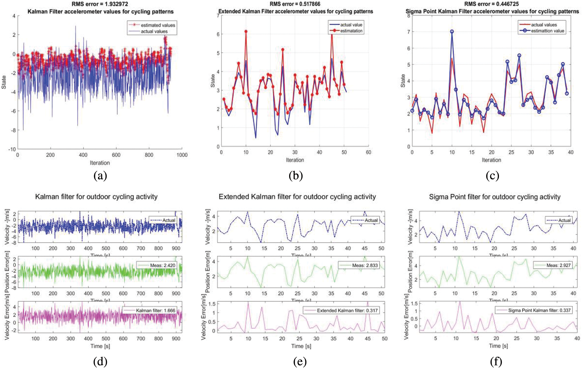
Figure 9: (a–c) Outdoor cycling activity for estimated and actual sensor data on KF, EKF, SPKF (d–f) velocity and position of the error activity on KF, EKF and SPKF

6.1 Indoor Condition for Sitting and Under-ground Activity

The experiment in indoor conditions is carried out for 30–45 min in both sitting and underground walking modes of the subject to calculate the acceleration and sensor predicted values on acceleration rate. The indoor prediction performance of the three variations of the Kalman filter on the accelerometer data is depicted in Figs. 8a–8c. This graph also demonstrates the performance of the Extended Kalman filter, Sigma point Kalman filter on sensor-based activities.

These figures also show the difference between the measured and the real position, as well as the difference between the KF, EKF and SPKF estimate and the real position. The number of data points is used to normalize the error in measuring and estimating the position. The estimation error of position and velocity is shown in the Figs. 8d–8f. The Kalman filter velocity estimates accurately the actual velocity trends. As the subject travels at high speeds, the noise level lowers. This is consistent with the covariance matrix’s design. The filter estimates catch up with the actual velocity after a few time steps. To depict the indoor activity outcome for the extended Kalman filter, and it was observed that the velocity error’s has decreased considerably. The fundamental concept underlying the SPKF algorithm is to apply unscented transformations to a set of sigma points representing a random variable in order to estimate the state in the subsequent step, or the output of the system, i.e., a measurement update. Figs. 8c and 8f depict the indoor activity outcome for the sigma point Kalman filter.

6.2 Outdoor Condition for Walking, Staircase-Down, Cycling and Staircase-Up Activity

The experiment is carried out in the subject’s walking, cycling, and staircase up and staircase down climbing modes for 30–45 min in order to calculate the acceleration and sensor predicted values on acceleration rate in the outdoor condition. The sample estimation plots for the cycling activity carried on the three estimators KF, EKF and SPKF is shown in Fig. 9

6.3 Comparisons of Sensor Value with Expected and Estimated Values with Variance

As the item is in motion, this gyroscope data will be analyzed using a non-linear method to compare actual gyroscope data with estimated sensor data values. The proposed system’s accuracy was estimated by calculating the root-mean-square (RMS) difference between the three-axis estimated accelerometer values from actual sensor values and the three projected angles obtained from the sensor MPU6050. The accelerometer and gyroscope data applied to the three variants, KF, EKF, and SPKF are displayed along with their real values, estimated values and variance in Table 4.

The root mean Square (RMS) values have been widely employed in the literature to evaluate the accuracy of the estimator by measuring the difference between the estimated values and the true values as shown in Table 5. To evaluate the efficacy of the proposed estimating setup, certain related and current research comparable with analogous system is used. Unlike the work presented in [34,35], which is carried out only in the regular operation mode of just an accelerometer and gyroscope with single data condition and estimation of values for IMU respectively, the suggested technique adapt both the sensor-based system and GPS-based. The proposed work has been tested for six exercise or tasks, for indoor and outdoor navigation with adequate set of samples, but only few are being displayed here.

It can be seen that the values of the accuracy indices as RMS values confirm the effectiveness of the estimator. To test the performance of the proposed estimation setup, some related and recent works are chosen for comparison with an equivalent system and setup. The methods reported in Refs. [10,13] are based on a technique that is equally effective in the normal operation mode of a GPS/INS integration with a Kalman filter for the navigation applications. The work reported in the Refs. [13,29] is related to the activity trajectory accounting with the SPKF and EKF to accommodate nonlinearities and asynchronous and lagging sensor measurements for the walking activity. The proposed work states the components of the KF, EKF, and SPKF for the subject activity in various navigation environments and it outperforms in accuracy.

7  Conclusions and Future Plan

Equipment, environment, and mistakes can all have an impact on navigation performance, but these factors are not the only ones to consider. It is not immediately possible to measure these contact forces and related dynamics; hence, it is necessary to infer these time-varying dynamics using the sensors already present in the system, using cutting-edge methods. This research focuses on understanding real-time dynamics of the sensor values and their influence on state estimator filters. The experimental results from this set up, analyze the performance of the Kalman filter, the Extended Kalman filter, and the Sigma Point Kalman filter. During the investigation, it was discovered that the Kalman filter has an accurate estimation and prediction of the state for non-linear indoor localization and tracking application, even though the sensor data comes from real-time sensors.

Experiments conducted on Kalman filtering indicate that when data is noiseless or trusted, estimation for prediction of data is more accurate, but the accelerometer is susceptible to noise, which causes estimation to fluctuate. The accelerometer itself provides a nonlinear, noisy reading. This nonlinearity may result in a loss of precision and hence an approach using randomness is proposed. In addressing it, process noise and sensor noise for state estimation are considered, resulting in a more accurate state estimate and improved covariance. Specifically, the EKF has an implied approximation at a single point, in contrast to the SPKF, which approximates at several places for greater precision. These sigma points have the same weighted mean and covariance as the random variables. The performance of the different versions of the Kalman filter is evaluated using accuracy indices and compared to other pertinent and recent studies. The sigma point state estimator not only validated the individual’s performance in conventional indoor ‘underground walking’ activity and outdoor ‘cycling’ activity, which also exhibited durability in rapidly-changing physical activities. SPKF is anticipated to perform better than KF and EKF.

This work contributes to the overall performance of linear and nonlinear filtering by introducing a sensor with high sensitivity at moderate level and an analysis of its drift over time. Sigma filter-based prediction and estimate techniques are numerical rather than analytical, which has many benefits:

1.    They provide a superior covariance approximation for state estimation.

2.    They are portable.

3.    Their computing cost is lower than that of the EKF, so there is no need for a fully trained model to execute and evaluate them.

Additional study would require converting the data prediction and estimation method to embedded hardware using an appropriate implementation procedure so that it can be implemented using a machine learning-based methodology. Additionally, new active and novel supervised and unsupervised learning methodologies must be investigated to create novel models for real-time prediction on hardware.

Funding Statement: The authors received no specific funding for this study.

Conflicts of Interest: The authors declare that they have no conflicts of interest to report regarding the present study.

References

1. M. Wright, D. Stallings and D. Dunn, “The effectiveness of global positioning system electronic navigation,” in Proc. of IEEE Southeast Conf., 2003, Ocho Rios, Jamaica, pp. 62–67, 2004. [Google Scholar]

2. K. Fallahi, C. Cheng and M. Fattouche, “Robust positioning systems in the presence of outliers under weak GPS signal conditions,” IEEE Systems Journal, vol. 6, no. 3, pp. 401–413, 2012. [Google Scholar]

3. G. Fornaro, N. D. Agostino, R. Giuliani, C. Noviello, D. Reale et al., “Assimilation of GPS-derived atmospheric propagation delay in DinSAR data processing,” IEEE Journal of Selected Topics in Applied Earth Observations and Remote Sensing, vol. 8, no. 2, pp. 784–799, 2015. [Google Scholar]

4. J. Kim, J. Song, H. No, D. Han, D. Kim et al., “Accuracy improvement of DGPS for low-cost single-frequency receiver using modified flächen korrektur parameter correction,” ISPRS International Journal of Geo-Information, vol. 6, no. 7, pp. 222–243, 2017. [Google Scholar]

5. M. Shao and X. Sui, “Study on differential GPS positioning methods,” in Int. Conf. on Computer Science and Mechanical Automation (CSMA), Hangzhou, China, pp. 223–225, 2015. [Google Scholar]

6. J. Farrell and T. Givargis, “Differential GPS reference station algorithm-design and analysis,” IEEE Transactions on Control Systems Technology, vol. 8, no. 3, pp. 519–531, 2020. [Google Scholar]

7. S. Godha and M. E. Cannon, “GPS/MEMS INS integrated system for navigation in urban areas,” GPS Solutions (2007), vol. 11, no. 3, pp. 193–203, 2007. [Google Scholar]

8. N. E. Sheimy and A. Youssef, “Inertial sensors technologies for navigation applications: State of the art and future trends,” Satellite Navigation, vol. 1, no. 1, pp. 1–21, 2020. [Google Scholar]

9. M. Zhong, J. Guo and Z. Yang, “On the real-time performance evaluation of the inertial sensors for INS/GPS integrated systems,” IEEE Sensors Journal, vol. 16, no. 17, pp. 6652–6661, 2016. [Google Scholar]

10. Z. Wu, Z. Sun, W. Zhang and Q. Chen, “A novel approach for attitude estimation based on MEMS inertial sensors using nonlinear complementary filters,” IEEE Sensors Journal, vol. 16, no. 10, pp. 3856–3864, 2016. [Google Scholar]

11. D. Chattaraj, K. B. M. Swamy and S. Sen, “Design and analysis of dual axis MEMS accelerometer,” in Int. Conf. on Electronics and Communication Systems (ICECS), Mumbai, India, pp. 718–720, 2007. [Google Scholar]

12. Z. Kowalczuk and T. Merta, “Evaluation of position estimation based on accelerometer data,” in Int. Workshop on Robot Motion and Control, Poznan, Poland, Poznan University of Technology, pp. 246–251, 2015. [Google Scholar]

13. J. Z. Sasiadek and P. Haryana, “GPS/INS sensor fusion for accurate positioning & navigation based on Kalman filter,” IFAC Proceedings Volumes, vol. 37, no. 5, pp. 115–220, 2004. [Google Scholar]

14. M. S. Grewal and A. P. Andrew, Kalman Filtering: Theory and Practice Using MATLAB, 2nd ed., New York, Unites States: John Wiley & sons, pp. 1–401, 2001. [Google Scholar]

15. C. Urrea and R. Agramonte, “Kalman filter: Historical overview and review of its use in robotics 60 years after its creation,” Journal of Sensors, vol. 2021, no. 5, pp. 1–21, 2021. [Google Scholar]

16. J. L. R. Lara, S. Salazar and R. Lozano, “Real-time localization of an UAV using Kalman filter and a wireless sensor network,” Journal of Intelligent & Robotic Systems, vol. 65, no. 1–4, pp. 283–293, 2011. [Google Scholar]

17. S. Qiu, Z. Wang, H. Zhao, K. Qin, Z. Li et al., “Inertial/magnetic sensor based pedestrian dead reckoning by means of multi-sensor fusion,” Information Fusion, vol. 39, no. 1, pp. 108–119, 2017. [Google Scholar]

18. H. Geng, Y. Liang, Y. Liu and F. E. Alsaadi, “Bias estimation for asynchronous multi-rate multi-sensor fusion with unknown inputs,” Information Fusion, vol. 39, no. 11, pp. 139–153, 2017. [Google Scholar]

19. K. Watanabe, K. Kobayashi and F. Munekata, “Multiple sensor fusion for navigation systems,” in Proc. of VNIS’94 Vehicle Navigation and Information Systems Conf., Yokohama, Japan, pp. 575–578, 1994. [Google Scholar]

20. S. Wang and W. Ren, “On the consistency and confidence of distributed dynamic state estimation in wireless sensor networks,” in 2015 IEEE 54th Annual Conf. on Decision and Control (CDC), Osaka, Japan, pp. 3069–3074, 2015. [Google Scholar]

21. S. Wang and W. Ren, “On the convergence conditions of distributed dynamic state estimation using sensor networks: A unified framework,” IEEE Transactions on Control Systems Technology, vol. 26, no. 4, pp. 1300–1316, 2018. [Google Scholar]

22. A. Kulkarni and A. S. Beulet, “Statistical analysis of accelerometer, gyroscope with state estimation,” International Journal of Engineering and Advanced Technology (IJEAT), vol. 9, no. 1S3, pp. 139– 143, 2019. [Google Scholar]

23. Y. Jiang, Y. Huang, W. Xue and H. Fang, “On designing consistent extended Kalman filter,” Journal of Systems Science and Complexity, vol. 30, no. 4, pp. 751–764, 2017. [Google Scholar]

24. W. Li, Y. Jia and J. Du, “Distributed extended Kalman filter with nonlinear consensus estimate,” Journal of the Franklin Institute, vol. 354, no. 17, pp. 7983–7995, 2017. [Google Scholar]

25. G. Reina and A. Messina, “Vehicle dynamics estimation via augmented extended Kalman filtering,” Measurement, vol. 133, no. 10, pp. 383–395, 2019. [Google Scholar]

26. H. H. A. Malki, A. I. Moustafa and M. H. Sinky, “An improving position method using extended Kalman filter,” Procedia Computer Science, vol. 182, no. 6, pp. 28–37, 2021. [Google Scholar]

27. M. A. Skoglund, G. Hendeby and D. Axehill, “Extended Kalman filter modifications based on an optimization view point,” in 2015 18th Int. Conf. on Information Fusion (Fusion), Washington, DC, USA, pp. 1856–1861, 2015. [Google Scholar]

28. L. Ma, N. Cao, X. Feng and M. Mao, “Indoor positioning algorithm based on maximum correntropy unscented information filter,” ISPRS International Journal of Geo-Information, vol. 10, no. 441, pp. 1–17, 2021. [Google Scholar]

29. R. V. D. Merwe and E. A. Wan, “Sigma-point Kalman filters for nonlinear estimation and sensor-fusion—applications to integrated navigation,” in AIAA Guidance, Navigation, and Control Conf., Providence, Rhode Island, pp. 1–30, 2004. [Google Scholar]

30. T. Beravs, J. Podobnik and M. Munih, “Three-axial accelerometer calibration using Kalman filter covariance matrix for online estimation of optimal sensor orientation,” IEEE Transactions on Instrumentation and Measurement, vol. 61, no. 9, pp. 2501–2511, 2012. [Google Scholar]

31. Y. Kim and H. Bang, ``Introduction to Kalman filter and its application," in Introduction and Implementations of the Kalman Filter, London, United Kingdom: IntechOpen, 2018. [Online]. Available at: https://www.intechopen.com/chapters/63164 [Google Scholar]

32. E. A. Wan and R. V. D. Merwe, “The unscented Kalman filter for nonlinear estimation,” in Proc. of IEEE 2000 Adaptive Systems for Signal Processing, Communications, and Control Symp. (Cat. No.00EX373), Lake Louise, AB, Canada, pp. 153–158, 2000. [Google Scholar]

33. R. Kandepu, B. Foss and L. Imsland, “Applying the unscented Kalman filter for nonlinear state estimation,” Journal of Process Control, vol. 18, no. 7–8, pp. 753–768, 2008. [Google Scholar]

34. R. I. A. A. Ma’arif and S. Sunardi, “Noise reduction in the accelerometer and gyroscope sensor with the Kalman filter algorithm,” Journal of Robotics and Control (JRC), vol. 2, no. 3, pp. 180–189, 2021. [Google Scholar]

35. J. Gross, Y. Gu, S. Gururajan, B. Seanor and M. R. Napolitano, “A comparison of extended kalman filter, sigma-point Kalman filter, and particle filter GPS/INS sensor fusion,” in AIAA Guidance, Navigation, and Control Conf., Toronto, Ontario, Canada, pp. 1–20, 2010. [Google Scholar]