
 Submit a Paper
 Propose a Special lssue
 Open Access
ARTICLE

A New Hybrid Feature Selection Sequence for Predicting Breast Cancer Survivability Using Clinical Datasets
Centre for Information Technology and Engineering, Manonmaniam Sundaranar University, Tirunelveli, India
* Corresponding Author: E. Jenifer Sweetlin. Email:
Intelligent Automation & Soft Computing 2023, 37(1), 343-367. https://doi.org/10.32604/iasc.2023.036742
Received 11 October 2022; Accepted 06 January 2023; Issue published 29 April 2023
 View Full Text
 Download PDF
Abstract
This paper proposes a hybrid feature selection sequence complemented with filter and wrapper concepts to improve the accuracy of Machine Learning (ML) based supervised classifiers for classifying the survivability of breast cancer patients into classes, living and deceased using METABRIC and Surveillance, Epidemiology and End Results (SEER) datasets. The ML-based classifiers used in the analysis are: Multiple Logistic Regression, K-Nearest Neighbors, Decision Tree, Random Forest, Support Vector Machine and Multilayer Perceptron. The workflow of the proposed ML algorithm sequence comprises the following stages: data cleaning, data balancing, feature selection via a filter and wrapper sequence, cross validation-based training, testing and performance evaluation. The results obtained are compared in terms of the following classification metrics: Accuracy, Precision, F1 score, True Positive Rate, True Negative Rate, False Positive Rate, False Negative Rate, Area under the Receiver Operating Characteristics curve, Area under the Precision-Recall curve and Mathews Correlation Coefficient. The comparison shows that the proposed feature selection sequence produces better results from all supervised classifiers than all other feature selection sequences considered in the analysis.Keywords
Breast cancer is a major cause of the increasing mortality rate among women aged less than 70 years in over 112 countries, as estimated by the World Health Organization in 2019 [1]. In India, although 70% of deceased patients belong to a higher age group of over 50 years, several adverse environmental conditions have further reduced the higher age limit to be affected by the disease to less than 40 years [2]. Women with breast cancer have fewer survival rates when the tumors are larger and at higher stages of growth. Tumor stage is directly related to the number of positive lymph nodes. Abnormalities in tumor cells at higher stages also adversely affect the survival of breast cancer patients. The cancer type also plays a decisive role in the survival of cancer patients [3]. The clinical features of breast cancer patients such as menopausal status, laterality of tumor origin and type of breast surgery which are not directly obtained from MRI scan images or mammograms are also responsible for the survival of breast cancer patients. Thus, by analyzing the correlation between these associated features, patient age, tumor stage, tumor size, cancer type, number of positive lymph nodes and tumor grade, the survivability of patients can be identified. Information regarding these features can be found in the clinical breast cancer datasets METABRIC [4] and Surveillance, Epidemiology and End Results (SEER). If the survivability of patients with breast cancer is predicted based on the aforementioned independent features, a later course of treatment can be suitably decided. Patients in a critical state of breast cancer experience serious side effects mental and physical trauma when subjected to treatments involving heavy dose chemotherapy or radiotherapy [5]. If the criticality of breast cancer for survivability can be determined, patients can be relieved from psychological and physical trauma due to treatment by deciding whether to start or end second-line treatment. Second-line palliative or hospice treatment can provide relief and improve the quality of later life [6]. So, this paper analyzes the information in the independent and dependent feature values of the METABRIC and SEER datasets to determine the survivability of breast cancer patients as living and deceased. This paper also proposes a distinct feature selection sequence in the Machine Learning (ML) workflow for a more accurate prediction of the survivability of breast cancer patients.
With the advent of big data computer technology and the availability of voluminous and multidimensional clinical health records of breast cancer patients in digital form, Artificial Intelligence systems based on Data Mining, ML and Deep Learning have evolved for accurate and efficient solutions in breast cancer diagnosis, prognosis, patient management and survivability prediction [7,8]. Many multidimensional clinical datasets contain independent features that may not be relevant for specific ML-based medical applications. Therefore, identifying more suitable independent features is essential for improving the performance of ML-based medical applications [9]. Data preprocessing, feature selection and feature extraction techniques are applied to large datasets to obtain more important features before designing ML-based classifiers, such as Multiple Logistic Regression (MLR), K-Nearest Neighbors (K-NN), Decision Tree (DT), Random Forest (RF), Support Vector Machine (SVM) and Neural Networks (NN) to improve prediction accuracy [10–12]. Data preprocessing techniques remove redundant, noisy and irrelevant features from datasets. Feature selection (FS) techniques create a subset of independent features from the original dataset, such that they are more correlated with the dependent feature. Feature extraction techniques create a new set of features from the original features of a dataset using functional mappings that simultaneously preserve the original data and maintain the relative distance between the features [13].
From the literature, it is observed that in ML papers [14–23], feature selection and extraction techniques applied before the training stage improve data visualization, prediction accuracy, reduce computing and storage requirements. Nilashi et al. [14] proposed a ML-based system combining Expectation Maximization (EM), Principal Component Analysis (PCA), Classification and Regression Tree (CART) and Fuzzy Rule (FR) based methods to increase the predictive accuracy of breast cancer classification using the Wisconsin Diagnostic Breast Cancer (WDBC) and Mammographic mass dataset. Solanki et al. [15] proposed a wrapper-based feature selection approach using Particle Swarm Optimization (PSO), Genetic Search (GS) and Greedy Stepwise methods with ML classifiers, SVM, DT and Multilayer Perceptron (MLP) on the WDBC dataset. The results showed that an accuracy of 98.83% was obtained when DT and RF are combined with GS for breast cancer prognosis. Dhahri et al. [16] constructed a system to accurately differentiate benign and malignant breast tumors based on Genetic Programming and classifiers such as SVM, K-NN, DT, Gradient Boosting classifier, RF, LR, AdaBoost (AB), Gaussian Naive Bayes and Linear Discriminant Analysis (LDA) using the WDBC dataset. The feature selection techniques used are Univariate Feature Selection (UFS) and Recursive Feature Elimination (RFE). The best accuracy, 98.24% was achieved using the AB classifier. Prince et al. [17] proposed an efficient ensemble method for breast cancer detection using Wisconsin Breast Cancer Database-Original (WBCD), WDBC and Wisconsin Lung Cancer Datasets (WLCD). Feature selection methods such as PCA, Pearson Correlation Coefficient (PCC) and Chi-Square (CS) are used to obtain common features from the feature sets using the set union operation. Classifiers such as Naive Bayes (NB), K-NN, DT, RF and SVM are used for classification. RF produced an accuracy of 97.4% and SVM produced an accuracy of 97.8%. Fogliatto et al. [18] proposed a combination of PCA and Bhattacharyya distance methods in the preprocessing stage to obtain a feature importance index. The classification techniques used are K-NN, LDA and Probabilistic Neural Network for classification of the WBCD dataset. K-NN produced higher accuracy.
Shukla et al. [19] predicted breast cancer survivability on the SEER dataset using unsupervised data mining methods, Self-Organizing Maps and Density-Based Spatial Clustering. The cluster patterns obtained are used to train the MLP model to improve the patient survivability. Information Gain (IG) was computed for feature selection. The prediction accuracy was 86.96%. Sedighi-Maman et al. [20] used Generalized Linear Model (GLM), Extreme Gradient Boosting, MLP classifiers and regression techniques on the SEER dataset to predict the survival status. The Least absolute shrinkage and selection operator and RF methods are used for the feature selection. The highest Area under the curve (AUC) value obtained was 90% when predicting survival status. Wang et al. [21] compared the performance of three classifiers, LR, DT and K-NN for the classification of survivability in patients with breast cancer. The Synthetic Minority Oversampling Technique (SMOTE) and PSO are used to solve the imbalance problem. The combination of SMOTE and PSO with DT yielded a high accuracy of 94.26%. Jahanbazi et al. [22] used the Adaboost.M1 algorithm and DT to predict breast cancer survival. SMOTE and IG are used for feature selection. The DT performed better with an accuracy of 87.07%. Boughorbel et al. [23] compared the performance of eight predictive models namely NN, SVM, RF, Boosted Trees, GLM, GLM-Elastic Net, K-NN and Partial Least Squares to predict the survivability of breast cancer for different prognosis periods based on the Area under the curve-Receiver operating characteristics (AUC-ROC) performance. RF performed with the highest AUC of 77%.
Based on the literature review, it is observed that feature selection techniques improve the accuracy of classifiers designed for the diagnosis of breast cancer and prediction of the survivability of breast cancer patients. It is found that although the papers, [14–18] used WDBC and WBCD datasets with data from MRI breast images and mammograms for the classification and diagnosis of breast cancer, many other clinical features of the patient such as age, laterality of tumor origin, menopausal status and type of breast surgery also play an important role in inducing breast cancer and thus in the prediction of survival in breast cancer patients as has been reported in the literature [24–27]. The METABRIC and SEER datasets have clinical independent features. Therefore, this paper proposes a novel hybrid feature selection sequence using filter and wrapper techniques to identify relevant features to predict the survivability of patients with breast cancer using the METABRIC and SEER datasets. The proposed work focuses only on the new feature selection sequence and comparison of the performance of supervised classifiers; thus, survival analysis models such as Cox proportional hazard models are not within the scope of this research. The new feature selection sequence is proposed by referring to the feature selection technique in the ML workflow of [17] which produced an accuracy of 97.8% while diagnosing breast cancer using the features of WDBC, WBCD and WLCD. The proposed hybrid approach also incorporates data balancing using the Synthetic Minority Oversampling Technique-Edited Nearest Neighbor (SMOTE-ENN). The training set is subjected to filter techniques, Mutual Information (MI) and CS and the union of all independent features from MI and CS is further optimized using the wrapper technique, RFE-DT. Six prominent ML classifiers, MLR, K-NN, DT, RF, SVM and MLP are used to classify the preprocessed data for the prediction of survivability of breast cancer patients and the results are compared in terms of the following classification metrics: Accuracy (ACC), Precision (PR), F1 score (F1), Recall/True Positive Rate (TPR), True Negative Rate (TNR), False Positive Rate (FPR), False Negative Rate (FNR), AUC-ROC, Area under the Precision-Recall curve (AUC-PR) and Mathews Correlation Coefficient (MCC) [28,29]. The results obtained with and without feature selection and after applying the filtering methods: MI and CS separately are also used in the comparative analysis. The comparative analysis is also performed between the results of the proposed feature selection sequence and those obtained from papers published by Nilashi et al. [14], Dhahri et al. [16], Prince et al. [17], Shukla et al. [19], Wang et al. [21] and Jahanbazi et al. [22] in terms of accuracy and Boughorbel et al. [23] in terms of AUC-ROC. The comparative analysis shows that the proposed feature selection sequence produces higher performance values than all other techniques and methods. The remainder of this paper is organized as follows: Section.2 explains the proposed methodology, Section.3 presents the experimental results and analysis and Section.4 summarizes the proposed work and future work plan.
The paper proposes a distinct feature selection sequence for records of clinical breast cancer datasets namely METABRIC and SEER to model classifiers for predicting the survivability of patients with breast cancer. This feature selection sequence and its subsequent stages are illustrated in the block diagram in Fig. 1. The data cleaning, data balancing steps of the data preprocessing stage and filter, wrapper techniques of the proposed feature selection sequence used in the workflow of the system for predicting the survivability of breast cancer patients are described in the following subsections.
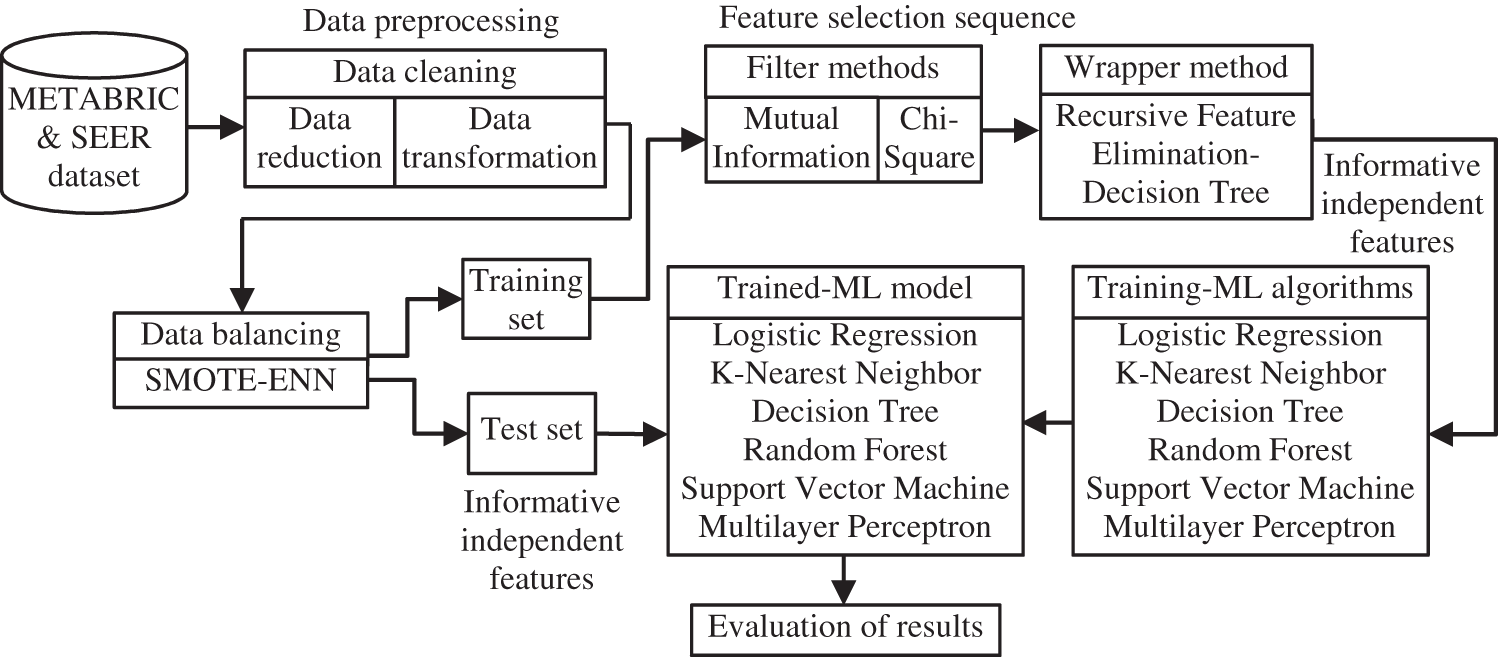
Figure 1: Work flow of the proposed feature selection sequence and later ML stages
In the proposed work, two clinical datasets, METABRIC and SEER are used for the experimental analysis. The METABRIC dataset is downloaded from cbioportal.org in .tsv (tab separated value) format. It has 2,509 data records with 38 features. The SEER dataset is an authentic source of cancer statistics supported by the Surveillance Research Program (SRP) of Cancer Control and Population Sciences (DCCPS), a division of the National Cancer Institute (NCI), USA and has been published on its website. The SEER registries are updated annually. It is downloaded in .slm (seer listing matrix) format with 7,755,157 records and 258 features. The records containing only breast cancer information are required for the analysis. All records corresponding to other types of cancer are removed from the SEER dataset. Therefore, the SEER dataset used in this paper has only 1,048,575 breast cancer records with 20 features. The features in the dataset have both numerical and categorical values.
Data cleaning is a significant step in preprocessing medical data in which data transformation and data reduction steps are performed. Data transformation techniques transform the data into a combined and uniform format. The downloaded METABRIC and SEER datasets are converted to .csv (comma separated value) format as needed for working in Python. Python is used to program the workflow of the proposed work. In the data reduction step, the relevant attributes are identified, and the records corresponding to missing, irrelevant and noisy data values are removed to improve the quality of the data [30]. During the data reduction step, records corresponding to the missing values of the independent and dependent features are removed. Instead of removing the records corresponding to null tumor stage values, considering the tumor size of the patients, the tumor stage values are replaced with relevant tumor stage values ranging from 1 to 4 as mentioned in the paper authored by Koh et al. [31] for the METABRIC dataset.
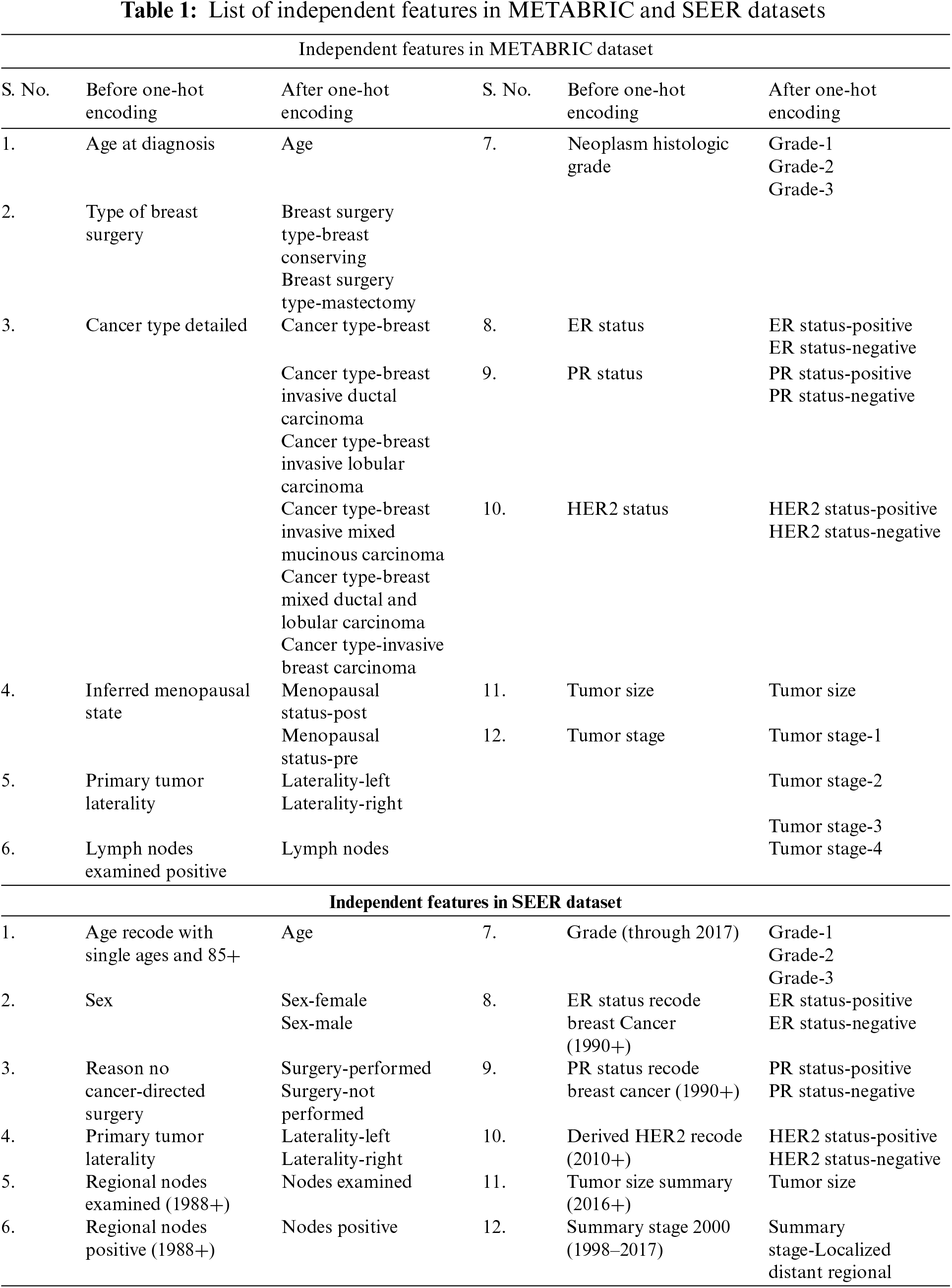
After applying these data cleaning steps to the METABRIC dataset, which originally had 2,509 records with 38 features, the dataset is reduced to 1,505 records with 12 independent features. Similarly, for the SEER dataset, 1,048,575 records with 20 features are cleaned to obtain 10,838 records with 12 independent features. The independent features are selected from the METABRIC and SEER datasets after consulting experts in the domain and are listed in Table 1. The dependent feature of the datasets is the survival status. The nominal categorical feature values of the datasets used in this work are converted into numerical values using the one-hot encoding technique [32]. After applying the one-hot encoding technique to the METABRIC dataset, the dataset has 1,505 records with 28 independent features and the SEER dataset has 10,838 records with 22 independent features. The increase in the number of independent features is because of the labels created for different independent features with categorical values as shown in Table 1. The second and fifth columns of Table 1. shows the independent features, whereas the third and sixth columns show those obtained after applying the one-hot encoding technique to the METABRIC and SEER datasets.
The predictive accuracy of a classification model is significantly affected when the dataset is imbalanced. The dataset is imbalanced when the number of records corresponding to different dependent feature values in the dataset is uneven, that is, an unbalanced dataset contains both minority and majority classes. Maximizing the overall accuracy is not the best approach with an imbalanced dataset, because the ML classifier focuses more on the majority class than on the minority class. This accuracy produces only misleading information regarding the minority classes. Therefore, the dataset must be balanced before it can be applied to classifiers [33,34]. In the proposed feature selection sequence, the SMOTE-ENN technique as mentioned in [35], is applied to address the imbalance in the dataset. It is a combination of two resampling techniques, SMOTE and ENN where SMOTE is an oversampling technique that generates synthetic data of minority samples according to their nearest neighbors. New samples are generated based on the difference between the feature vectors of the sample and their nearest neighbors. However, SMOTE is likely to generate noisy samples in the minority classes. Therefore, ENN is applied along with SMOTE where irrelevant noisy records are removed by comparing the dependent feature value of the records under consideration and the labels of their k-nearest neighbors. The records are removed if the dependent feature values are different [36].
In the METABRIC dataset, there are 868 records corresponding to the dependent feature value, deceased and 637 records corresponding to the dependent feature value, living. In the SEER dataset, there are 10,570 records corresponding to the dependent feature value, living and 268 records corresponding to the dependent feature value, deceased. After applying the SMOTE-ENN technique to both classes of METABRIC and SEER datasets, the imbalanced datasets are converted to balanced datasets. After data balancing, 279 records corresponding to the majority class, deceased and 346 records corresponding to the minority class, living are obtained for the METABRIC dataset. Similarly, 8,769 records corresponding to the majority class, living and 10,233 records corresponding to the minority class, deceased are obtained for the SEER dataset. The datasets are then split into 80% training set and 20% testing set.
When the datasets have a large number of independent features, associating all independent features with the dependent feature only reduces the accuracy of the ML classifier because all independent features of the training set are less associated with the dependent feature. Therefore, to reduce the dimensionality of the training set, eliminating less significant independent features produces more accurate classifiers. The selection of a few important independent features will also reduce the computational and storage expenses required for ML modeling. From the training set, feature selection techniques select a valuable feature subset to produce better classification results [37]. Feature selection techniques used for optimal feature selection are classified as filter, wrapper and embedded methods [38]. The ranking technique is the principal criterion of filter methods in which features are ranked based on relevant statistical scores. The ranking method filters out irrelevant independent features that have poor association with the dependent features from the dataset. Filter approaches are scalable and independent of ML algorithms [39]. The filter methods used in the proposed ML workflow are the MI and CS methods. These are implemented on the training sets of the METABRIC and SEER datasets using the scikit-learn library in Python. The methods are detailed as follows:
Mutual information [40] is a filtering method that helps to determine the dependency between independent and dependent features. The training sets used in this paper consists of many clinical features of breast cancer patients as independent features and the survival status of the patients as the dependent feature. The different independent features in the training set are denoted by
In Eq. (1),
where p(b) is the probability of a value b of
Here,
Chi-Square is a statistical measure [43,44] used to evaluate the relationship between two categorical or nominal independent and dependent features,
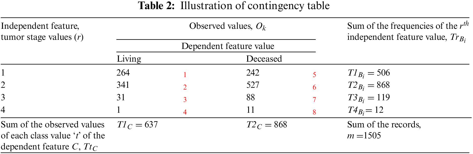
The expected value,
Here,
The
If the
Wrapper techniques identify independent features that are more correlated with the dependent feature by applying the independent features in the training set to simple classifiers and selecting the features which produce better classification. If the dimensionality of a dataset is high, wrapper methods are expensive in terms of time and computing resources because each feature set considered must be evaluated using the classifier. There are fewer independent features in the datasets used in the proposed work. Therefore, in the proposed feature selection sequence, the features detected by the filter method are applied to the wrapper method to identify more informative independent features. RFE is a widely used wrapper method for choosing independent features that are most related to the dependent feature of a classification problem [45–47].
RFE applies a backward selection process to find the optimal combination of features by analyzing the performance of classifiers such as RF, DT, SVM and LR [48]. In the proposed work, RFE is combined with a DT classifier [49] and applied to the independent features obtained using the filter method to identify more informative independent features. RFE with DT uses an iterative approach as shown in Fig. 2.
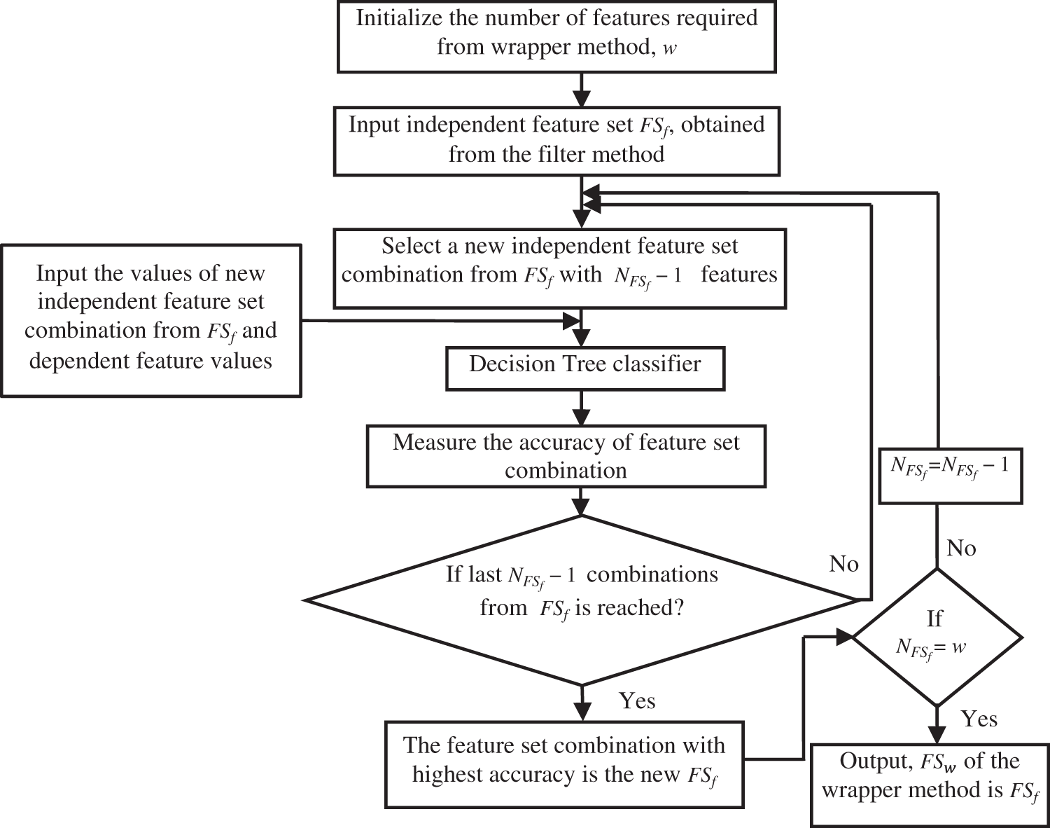
Figure 2: Working of Recursive Feature Elimination
In this approach, the number of independent features, ‘
Cross Validation-Based Training and Testing of ML Classifiers
In the ML domain, classification algorithms learn from labeled training data and the obtained model is used in the testing phase to determine the dependent feature value of the test record. The size of the training set and the predictive performance are positively correlated. In addition, a more accurate classification due to the empirical risk of overfitting can be reduced by cross-validation (CV) [50,51]. In the proposed work, a 10-fold CV is used, where to find the best model, the training set corresponding to the independent features obtained from the wrapper method is split into nine different training sets and a validation set. This validation set is used to determine the training accuracies of different classifiers produced after training. The training set is subjected to six ML classifiers [15,16] in the literature, such as MLR, K-NN, DT, RF, SVM and MLP for the classification of dependent feature values in METABRIC and SEER as living and deceased. In the following subsections, the training and testing phases of the different ML algorithms used in the performance analysis of the proposed feature selection sequence are presented.
2.6.1 Multiple Logistic Regression
Logistic Regression is used to solve binary classification problems when the dependent feature is categorical. The logistic regression used in the proposed work is MLR [52] because there are many independent features in the training set. As the name suggests, logistic regression has a logistic function, also called the sigmoid function, to predict the probability of the values of the dependent feature, living and deceased. The predictive function yields a probability value that ranges from zero to one. To classify the dependent feature values, the algorithm determines the best set of coefficients for the MLR model using different independent features identified in the proposed feature selection sequence. The MLR model is used to determine the probability of any test record having independent feature values. The class labels, living and deceased are identified as labels above or below a probability of 0.5 [53].
The K-Nearest Neighbor algorithm [54] is a supervised ML algorithm that identifies the label of a particular test record of independent features by finding its nearest neighbor class among the labels of the training records. The closest class of the test record is determined as the mode of ‘K’ smallest distance measures found between the incoming test record and all the records in the training set. The distance between each training record and the test record is calculated using the Euclidean, Manhattan, Chebyshev, Minkowski, or Hamming distances [55]. In the proposed work, the Manhattan distance is used to classify the test records into living and deceased classes because it produces fewer False Negative (FN) values.
Decision Tree [56] is a supervised learning algorithm that computes the relationship between independent and dependent features in a tree-like structure. The algorithm accounts for all records of the training set in the root node of the decision tree. The root node branches to specific internal nodes or terminal nodes based on the conditions to be satisfied for different values of independent features that are selected based on measurements of information content in the independent features: Goodness of fit measure [57], Gini index or Entropy or IG [58]. The decision tree splits until no further splitting of internal nodes is possible or when the decisions for the dependent feature values of all the records in the training set are made. Different independent features with different branches and levels of a decision tree provide a set of rules. These decision rules determine the dependent feature values of the test records as living or deceased during the testing phase.
Random Forest [59] is an ensemble supervised learning technique that works on many decision trees produced from different subsets of a given training set. The mode of prediction created by the different decision trees is the label of the test record. The prediction made by RF has a higher accuracy than that of decision trees. The more the number of decision trees in the forest, the greater the accuracy. RF also prevents overfitting and facilitates parallel processing [60].
Support Vector Machine [61] is a supervised learning algorithm whose training phase segregates an n-dimensional space of independent features using a hyperplane into two classes of the dependent feature by considering all training records. After the training phase, the coefficients of the best hyperplane separating the two class labels are obtained, such that the distance between the support vectors on either side of the best hyperplane provides the maximum margin. The extreme independent data records closest to the hyperplane are support vectors [62]. The best hyperplane model produced in the training phase for the clinical datasets METABRIC and SEER is used to classify the test records as living or deceased.
From literature [25], it is found that MLP is used to classify the survivability of patients with breast cancer. MLP is a feed-forward network in which the input layer of neurons acts as a receiver, one or more hidden layers of neurons compute intermediate inputs based on an activation function and the output layer predicts the output [63]. The number of input neurons corresponds to the number of independent features and the number of neurons in the output layer corresponds to the number of dependent feature values or class labels. The hidden layer produces an output based on the sigmoid function using the sum of the products of the inputs and the corresponding weights of the links from the input neuron to the respective hidden neuron. The number of hidden layers is chosen as a trade-off between performance and computational complexity. The weights of the links connecting the input and hidden, hidden and output layers are optimized during back-propagation based training [64] to obtain more accurate dependent feature values. The weights are updated during each training iteration based on the error between the actual and predicted outputs. The learning coefficient is set to a suitable value between zero and one for the convergence of the training phase. After training, the optimized weight matrix is tested using the test data. The experimental results and performance analysis of ML classifiers are discussed in the next section.
3 Experimental Results and Analysis
The proposed feature selection sequence is implemented in Python scikit-learn library on an Intel i5, 10th generation laptop at 1.19 GHz with 8 GB RAM. In this proposed work, two datasets, METABRIC and SEER are used for the experimental analysis. The datasets are subjected to a data preprocessing stage and the proposed feature selection sequence. In the data preprocessing step, data reduction, data transformation and data balancing steps are performed and the details of the preprocessed datasets are listed in Table 1. The filter techniques of the proposed feature selection sequence, MI and CS are applied to the preprocessed training sets. The more relevant independent features identified from the filter stage are subjected to the RFE-DT based wrapper technique to obtain the optimal set of independent features. The METABRIC and SEER datasets with independent features obtained after these filter and wrapper stages along with dependent feature, survival status are subjected to the ML algorithms mentioned in subsection 2.6 of Section.2 for obtaining the classification models to classify the test records in the test set into the class labels: living or deceased. The performance of the respective classifiers is analyzed in this section in terms of the following evaluation metrics: ACC, PR, F1, TPR, TNR, FPR, FNR, AUC-ROC, AUC-PR and MCC.
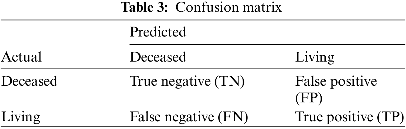
The performance of the classifiers is evaluated on the basis of their correct and incorrect predictions made by them. The confusion matrix for the classifier as shown in Table 3. is a report of correctly and incorrectly predicted labels in terms of True positive (TP), True negative (TN), False positive (FP) and False negative (FN). TP is the count of ‘living’ predicted by the classifier correctly while FP is the count of ‘deceased’ incorrectly predicted as ‘living’. TN is the count of ‘deceased’ predicted by the classifier correctly and FN is the count of ‘living’ predicted incorrectly as ‘deceased’. The objective metrics used in the analysis namely ACC, PR, F1, TPR, TNR, FPR, FNR, AUC-ROC, AUC-PR and MCC are defined in [28,35,45] based on these elements in the confusion matrix.
The results obtained from the different stages of the proposed feature selection sequence are presented below. To select 10 and 15 relevant independent features for the experimental analysis, the
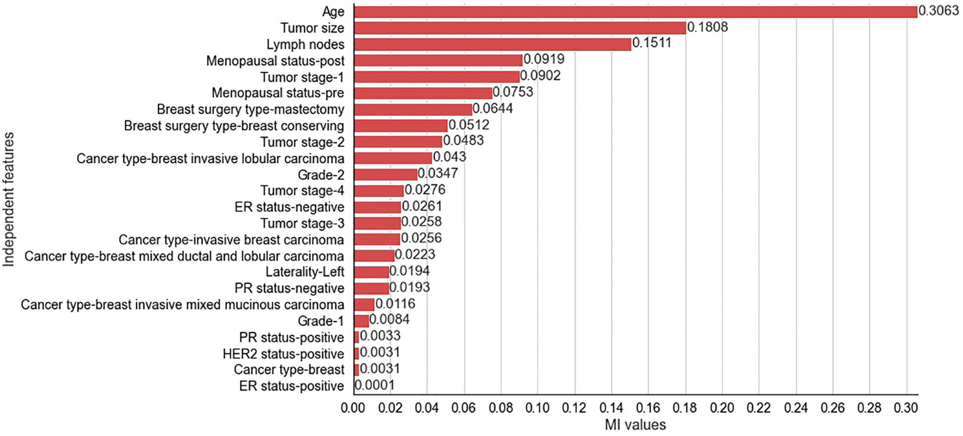
Figure 3: Mutual Information values for selected independent features for METABRIC dataset
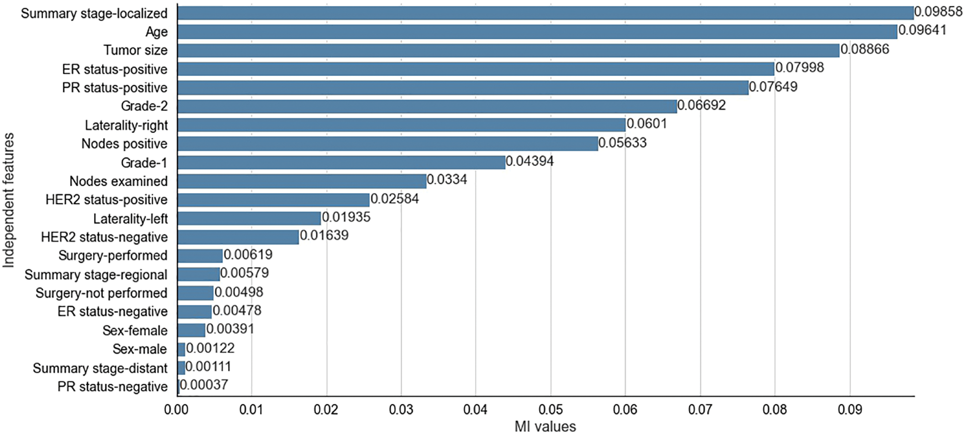
Figure 4: Mutual Information values for selected independent features for SEER dataset
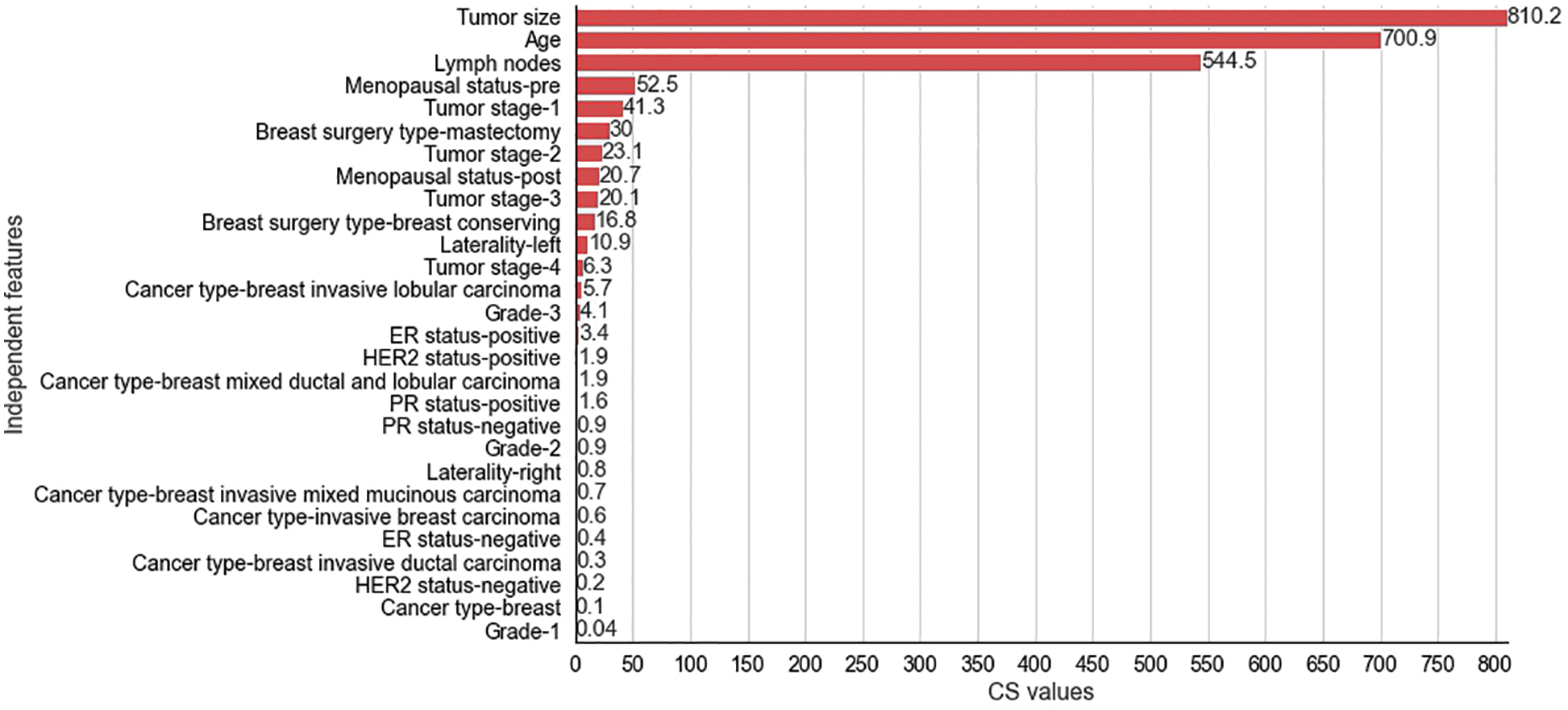
Figure 5: Chi-Square values for selected independent features for METABRIC dataset
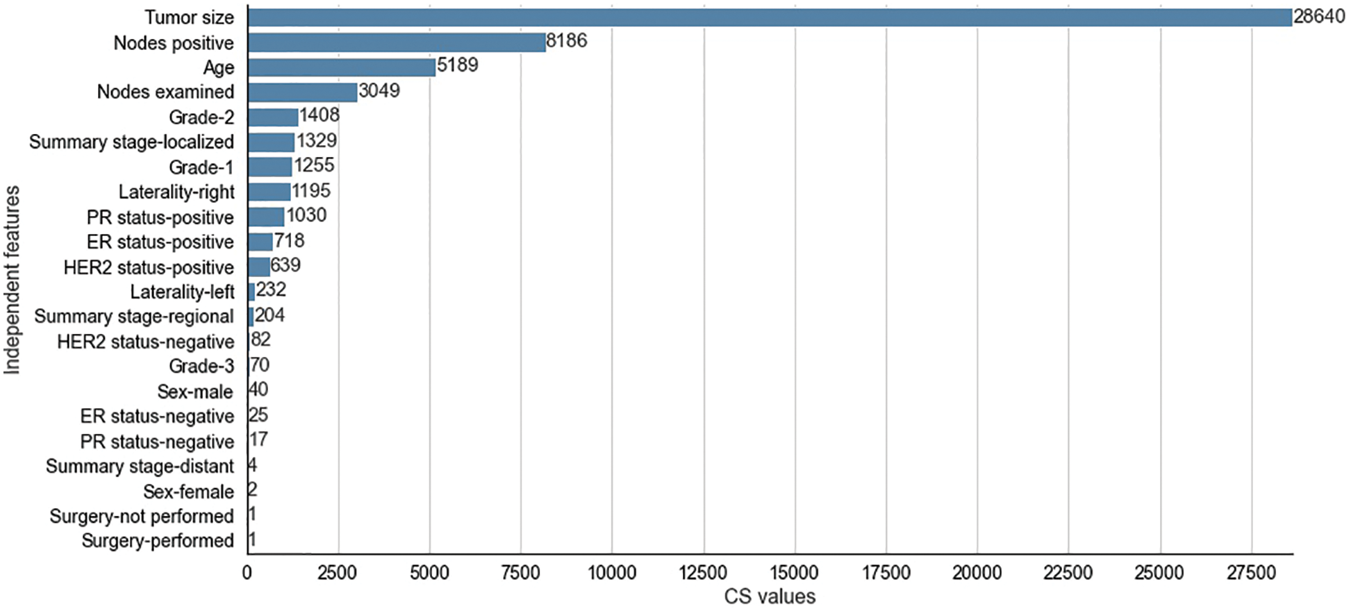
Figure 6: Chi-Square values for selected independent features for SEER dataset
The CS values produced by the CS filter from the independent and dependent features of the METABRIC and SEER datasets are shown in Figs. 5 and 6 respectively. The y-axis shows the selected
The two filter methods identified age, tumor size, number of positive lymph nodes, menopausal status, type of breast surgery and laterality of tumor origin as common and significant independent features in the proposed feature selection sequence for classifying patients with breast cancer from the METABRIC and SEER datasets. However, the different independent features that are highly correlated with the dependent feature, as identified by the MI and CS filters of the proposed feature selection sequence and the clinical features of breast cancer patients such as age, menopausal status, type of breast surgery and laterality of tumor origin, cannot be directly obtained from MRI scan images or mammograms. Therefore, analysis of clinical breast cancer data is important for predicting the survival of patients with breast cancer.
The informative set of independent features obtained from the two filter methods, MI and CS are applied to the RFE-DT wrapper method to obtain the optimal set of features. The top-ranking 10 and 15 independent features obtained after applying the RFE-DT wrapper method to the proposed feature selection sequence are listed in Table 4. for the METABRIC and SEER datasets, respectively.
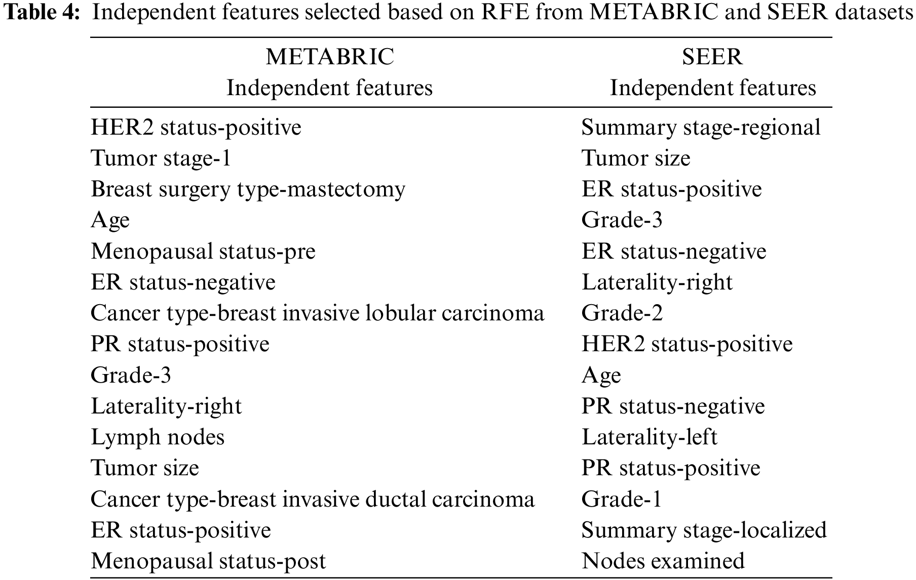
The training set corresponding to the independent features selected from the RFE-DT wrapper method is subjected to the training phase of six ML algorithms, MLR, K-NN, DT, RF, SVM and MLP. Of the independent features listed in Table 4, two optimal independent feature sets with 10 and 15 features each are assigned to the six ML algorithms along with their dependent feature values, living and deceased, to model the classifier and analyze the test performance of each classifier in terms of the evaluation metrics: ACC, PR, F1, TPR, TNR, FPR, FNR, AUC-ROC, AUC-PR and MCC. The values of the metrics obtained from the various ML classifiers used in the comparative analysis of the METABRIC and SEER test sets are listed in Table 5.
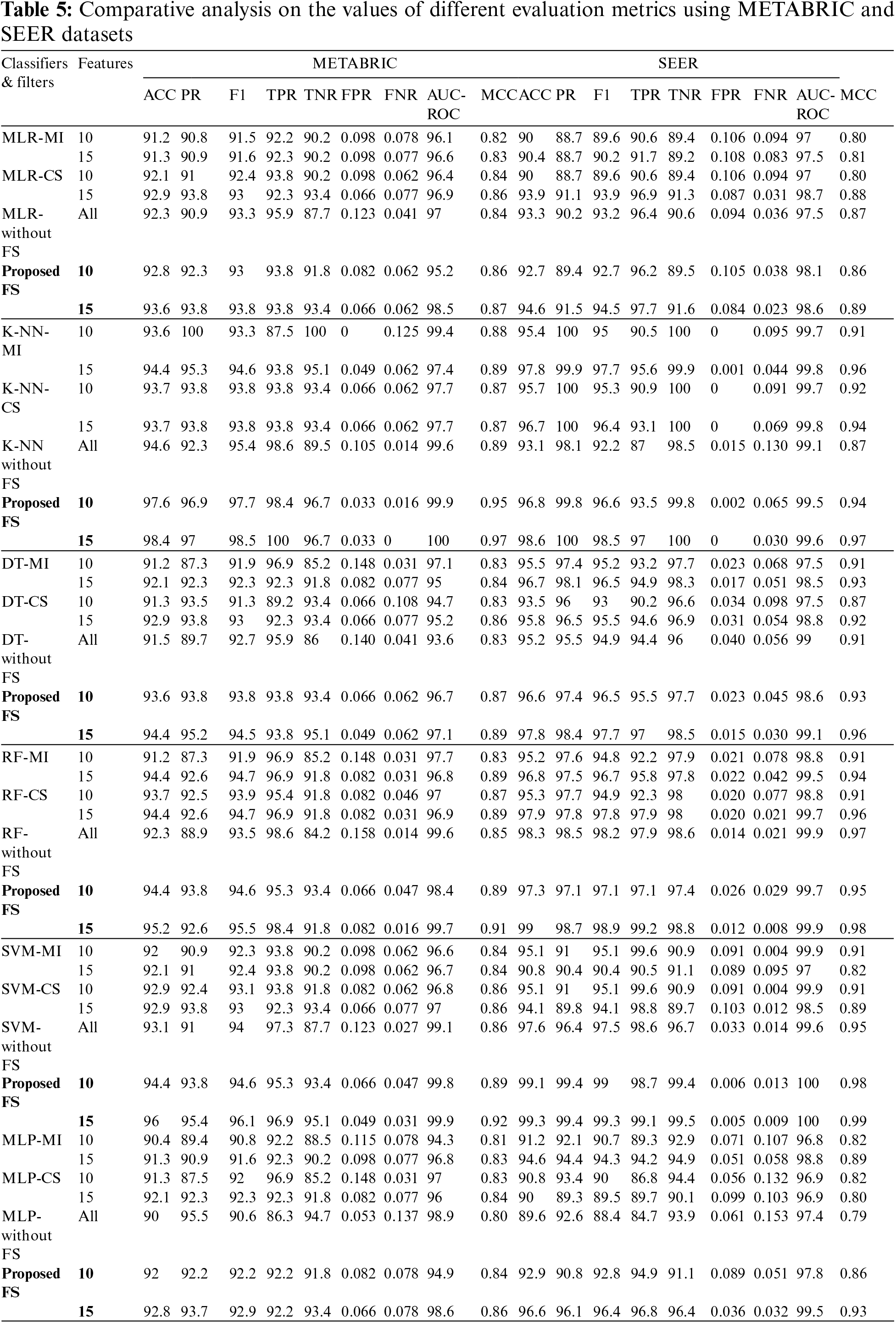
As shown in Table 5, when the proposed feature selection sequence is used, all the ML classifiers used in the comparative analysis produced higher values for ACC, PR, F1, TPR, TNR, FPR, FNR, AUC-ROC, AUC-PR and MCC than when the filter techniques, MI or CS were applied separately. When compared to all other ML classifiers used in the analysis, K-NN produced higher values for all evaluation metrics from the METABRIC test set when using the proposed feature selection sequence. SVM with the proposed feature selection sequence obtained the highest values for all the evaluation metrics from the SEER test set. The comparison shows a clear increase in accuracy for the METABRIC dataset from 0.7% to 4.7% and an increase in accuracy for the SEER dataset from 1.1% to 8.5%. A comparison is also made with the results produced by the ML classifiers without feature selection, as shown in Table 5. There is a clear increase in accuracy from 0.5% to 3.8% for the METABRIC dataset and an increase in accuracy from 1% to 7% for the SEER dataset.
The ROC and PR curves are drawn between FPR, TPR and Recall/TPR, Precision respectively. When the model predicts the probability of belonging to different classes, curves are plotted for different thresholds of the ML models under comparison. The ROC curves are plotted between FPR and TPR for the classifiers, MLR, K-NN, DT, RF, SVM and MLP corresponding to the proposed feature selection sequence for 15 independent features from the METABRIC and SEER datasets, respectively, as shown in Figs. 7a and 7b. The Area under ROC curves are higher for the ML classifiers when 15 independent features identified from the proposed feature selection sequence are used. According to Figs. 7a and 7b, the Area under the ROC curve of the K-NN and SVM classifiers is larger for the METABRIC and SEER datasets, respectively. The PR curves as shown in Figs. 8a and 8b are plotted between Recall and Precision for the classifiers, MLR, K-NN, DT, RF, SVM and MLP corresponding to the proposed feature selection sequence for 15 independent features from the METABRIC and SEER datasets respectively. The Area under PR curves are higher for the ML classifiers when 15 independent features identified from the proposed feature selection sequence are used. According to Figs. 8a and 8b, the Area under the PR curve of the SVM classifier is higher for both the METABRIC and SEER datasets.
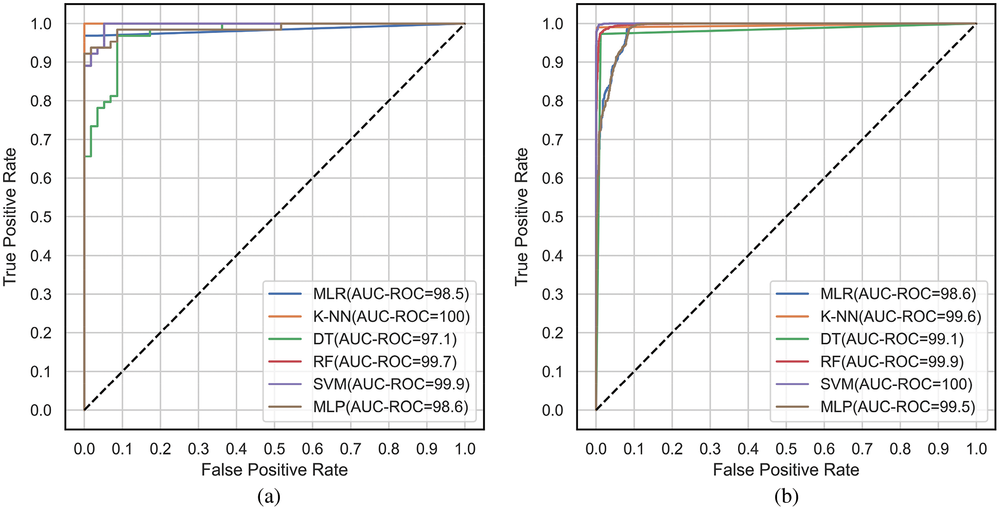
Figure 7: ROC curves for the proposed feature selection sequence with 15 independent features (a) METABRIC (b) SEER dataset
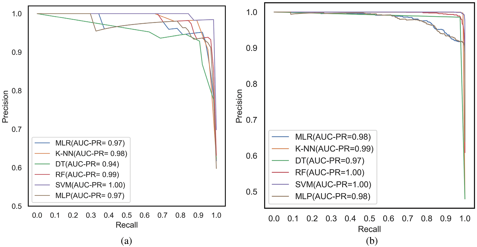
Figure 8: PR curves for the proposed feature selection sequence with 15 independent features (a) METABRIC (b) SEER dataset
The PR curves shown in Figs. 9a and 9b are plotted between Recall and Precision for the classifier, SVM, corresponding to the two filter methods, MI and CS applied separately, without feature selection, and the proposed feature selection sequence for 15 independent features from the METABRIC and SEER datasets, respectively. When 15 independent features identified from the proposed feature selection sequence are used, the SVM classifier has a higher Area under the PR curve.
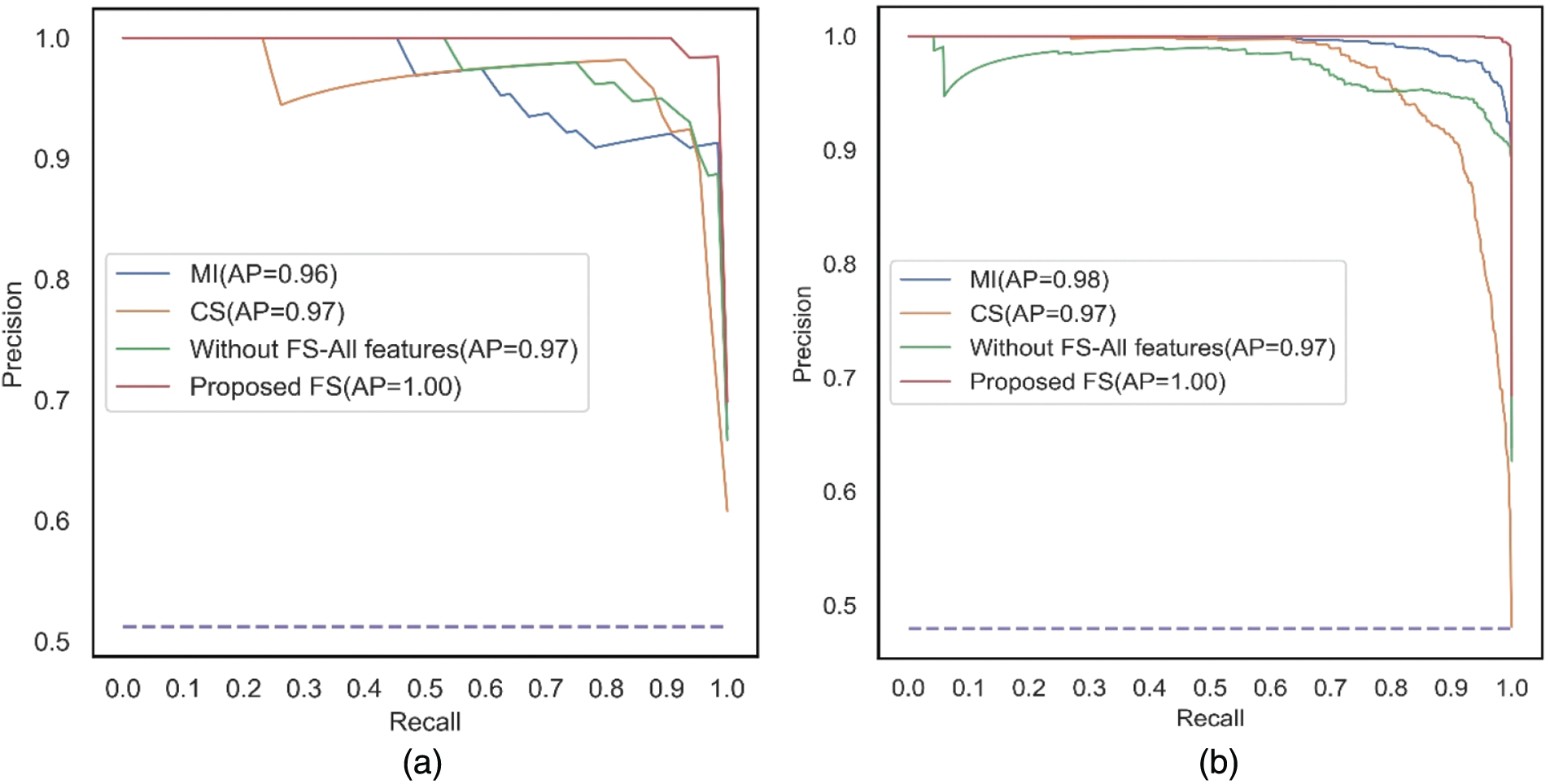
Figure 9: PR curves for all the comparative methods using SVM with 15 independent features (a) METABRIC (b) SEER dataset
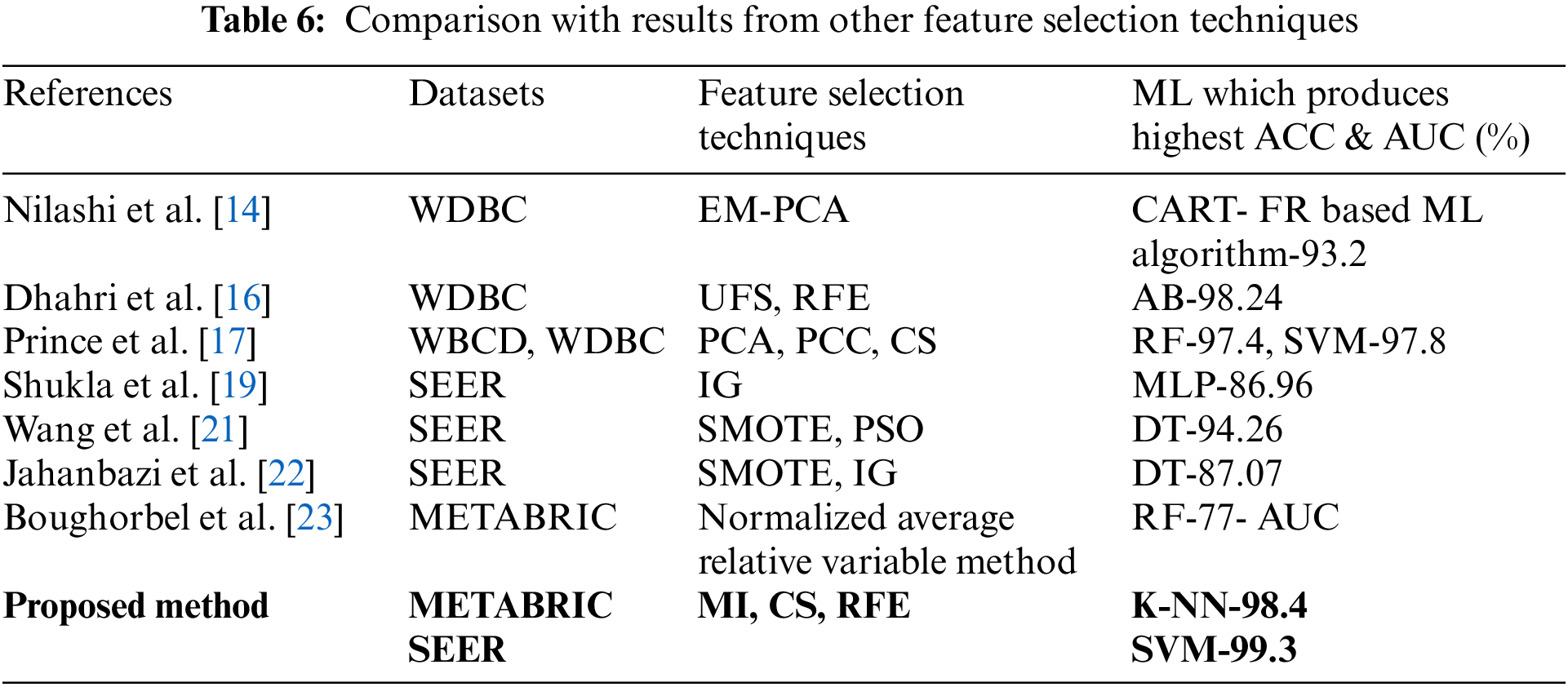
In addition, the proposed feature selection sequence results are compared with the results obtained in previous studies [14,16,17,19,21–23] which used the respective feature selection sequences as listed in Table 6. The accuracy produced by the feature selection techniques in [19,21] and [22] based on SEER is less than the results produced by the proposed feature selection sequence. Prince et al. [17] used PCC and CS in a feature selection sequence along with PCA for WDBC and WBCD datasets. The accuracies obtained were 97.4% for RF and 97.8% for SVM when compared to the accuracies produced by the proposed feature selection sequence which are 98.4% for K-NN and 99.3% for SVM from the METABRIC and SEER datasets, respectively. Thus, the proposed feature selection sequence outperformed all other feature selection sequences used in the comparative analysis when predicting the survivability of breast cancer patients using the ML algorithms, MLR, K-NN, DT, RF, SVM and MLP for the METABRIC and SEER datasets.
A new hybrid feature selection sequence is proposed to predict the survivability of breast cancer patients using the METABRIC and SEER datasets. The filter methods MI and CS are used along with the wrapper method, RFE-DT in the proposed feature selection sequence. The performance of the proposed feature selection sequence is analyzed for ML classifiers such as MLR, K-NN, DT, RF, SVM and MLP using the evaluation metrics, ACC, PR, F1, TPR, TNR, FPR, FNR, AUC-ROC, AUC-PR and MCC. The optimal features obtained from the proposed feature selection sequence are applied to the ML algorithms under analysis for training, and the test results obtained are compared with those obtained when ML classifiers are applied without any feature selection sequence and after applying the filtering methods, MI and CS separately. In addition, the results are compared with those obtained using other feature selection techniques. It is found that the proposed feature selection sequence produced higher values for all evaluation metrics when compared to other feature selection techniques in the comparative study while predicting the survivability of breast cancer patients. The few exceptional values of the metrics are to be explored in the later part of the research. This work can be extended to analyze the performance of other filter-wrapper combinations and ensemble techniques.
Acknowledgement: We express our sincere thanks to Prof. Dr. K. Rajendra Retnam, Former Dean, at Tirunelveli Medical College, Tamil Nadu, India, for guiding us in selecting features from the METABRIC and SEER dataset.
Funding Statement: The authors received no specific funding for this work.
Availability of Data and Materials:: The SEER dataset used in this work is taken from the SEER website and is available at the Surveillance Research Program, National Cancer Institute SEER*Stat software (seer.cancer.gov/seerstat) version 8.3.9.
Conflicts of Interest: The authors declare that they have no conflicts of interest to report regarding the present study.
References
1. H. Sung, J. Ferlay, R. L. Siegel, M. Laversanne, I. Soerjomataram et al., “Global cancer statistics 2020: GLOBOCAN estimates of incidence and mortality worldwide for 36 cancers in 185 countries,” CA: A Cancer Journal for Clinicians, vol. 71, no. 3, pp. 209–249, 2021. [Google Scholar] [PubMed]
2. S. S. Rajendran, P. K. Naik, S. Shankar, N. Asaithambi, S. S. Arunachalam et al., “Female breast cancer survivor’s perspectives on hope and spirituality needs-a mixed study approach,” Psychology and Education Journal, vol. 58, no. 2, pp. 9771–9780, 2021. [Google Scholar]
3. E. J. Sweetlin and S. Saudia, “Exploratory data analysis on breast cancer dataset about survivability and recurrence,” in Proc. IEEE Int. Conf. on Signal Processing and Communication, Coimbatore, India, pp. 304–308, 2021. [Google Scholar]
4. E. Cerami, J. Gao, U. Dogrusoz, B. E. Gross, S. O. Sumer et al., “The cBio cancer genomics portal: An open platform for exploring multidimensional cancer genomics data,” Cancer Discovery, vol. 2, no. 5, pp. 401–404, 2012. [Google Scholar] [PubMed]
5. A. Lahousse, E. Roose, L. Leysen, S. T. Yilmaz, K. Mostaqim et al., “Lifestyle and pain following cancer: State-of-the-art and future directions,” Journal of Clinical Medicine, vol. 11, no. 1, pp. 195, 2021. [Google Scholar] [PubMed]
6. M. Petrova, G. Wong, I. Kuhn, I. Wellwood and S. Barclay, “Timely community palliative and end-of-life care: A realist synthesis,” BMJ Supportive & Palliative Care, vol. 20, pp. 1–15, 2021. [Google Scholar]
7. A. Smiti, “When machine learning meets medical world: Current status and future challenges,” Computer Science Review, vol. 37, no. 3, pp. 100280, 2020. [Google Scholar]
8. D. Ben-Israel, W. B. Jacobs, S. Casha, S. Lang, W. H. A. Ryu et al., “The impact of machine learning on patient care: A systematic review,” Artificial Intelligence in Medicine, vol. 103, pp. 101785, 2020. [Google Scholar] [PubMed]
9. R. Dhanya, I. R. Paul, S. S. Akula, M. Sivakumar and J. J. Nair, “A comparative study for breast cancer prediction using machine learning and feature selection,” in Proc. IEEE Int. Conf. on Intelligent Computing and Control Systems, Madurai, India, pp. 1049–1055, 2019. [Google Scholar]
10. A. U. Haq, J. P. Li, M. H. Memon, S. Nazir, R. Sunet et al., “A hybrid intelligent system framework for the prediction of heart disease using machine learning algorithms,” Mobile Information Systems, vol. 2018, no. 8, pp. 1–21, 2018. [Google Scholar]
11. M. D. Ganggayah, N. A. Taib, Y. C. Har, P. Lio and S. K. Dhillon, “Predicting factors for survival of breast cancer patients using machine learning techniques,” BMC Medical Informatics and Decision Making, vol. 19, no. 1, pp. 1–17, 2019. [Google Scholar]
12. B. Zheng, S. W. Yoon and S. S. Lam, “Breast cancer diagnosis based on feature extraction using a hybrid of K-means and support vector machine algorithms,” Expert Systems with Applications, vol. 41, no. 4, pp. 1476–1482, 2014. [Google Scholar]
13. M. Li, H. Wang, L. Yang, Y. Liang, Z. Shang et al., “Fast hybrid dimensionality reduction method for classification based on feature selection and grouped feature extraction,” Expert Systems with Applications, vol. 150, pp. 113277, 2020. [Google Scholar]
14. M. Nilashi, O. Ibrahim, H. Ahmadi and L. Shahmoradi, “A knowledge-based system for breast cancer classification using fuzzy logic method,” Telematics and Informatics, vol. 34, no. 4, pp. 133–144, 2017. [Google Scholar]
15. Y. S. Solanki, P. Chakrabarti, M. Jasinski, Z. Leonowicz, V. Bolshev et al., “A hybrid supervised machine learning classifier system for breast cancer prognosis using feature selection and data imbalance handling approaches,” Electronics, vol. 10, no. 6, pp. 699, 2021. [Google Scholar]
16. H. Dhahri, E. Al Maghayreh, A. Mahmood, W. Elkilani and M. Faisal Nagi, “Automated breast cancer diagnosis based on machine learning algorithms,” Journal of Healthcare Engineering, vol. 2019, no. 12, pp. 1–11, 2019. [Google Scholar]
17. M. S. Prince, A. Hasan and F. M. Shah, “An efficient ensemble method for cancer detection,” in Proc. IEEE Int. Conf. on Advances in Science, Dhaka, Bangladesh, pp. 1–6, 2019. [Google Scholar]
18. F. S. Fogliatto, M. J. Anzanello, F. Soares and P. G. Brust-Renck, “Decision support for breast cancer detection: Classification improvement through feature selection,” Cancer Control, vol. 26, no. 1, pp. 1–8, 2019. [Google Scholar]
19. N. Shukla, M. Hagenbuchner, K. T. Win and J. Yang, “Breast cancer data analysis for survivability studies and prediction,” Computer Methods and Programs in Biomedicine, vol. 155, pp. 199–208, 2018. [Google Scholar] [PubMed]
20. Z. Sedighi-Maman and A. Mondello, “A two-stage modelling approach for breast cancer survivability prediction,” International Journal of Medical Informatics, vol. 149, pp. 104438, 2021. [Google Scholar] [PubMed]
21. K. J. Wang, B. Makond, K. H. Chen and K. M. Wang, “A hybrid classifier combining SMOTE with PSO to estimate 5-year survivability of breast cancer patients,” Applied Soft Computing, vol. 20, no. 3, pp. 15–24, 2014. [Google Scholar]
22. T. Jahanbazi and M. H. Nadimi, “An efficient method for predicting the 5-year survivability of breast cancer,” International Journal of Computer Applications, vol. 155, no. 8, pp. 8887, 2016. [Google Scholar]
23. S. Boughorbel, R. Al-Ali and N. Elkum, “Model comparison for breast cancer prognosis based on clinical data,” PLoS One, vol. 11, no. 1, pp. 146413, 2016. [Google Scholar]
24. S. Cai, W. Zuo, X. Lu, Z. Gou, Y. Zhou et al., “The prognostic impact of age at diagnosis upon breast cancer of different immunohistochemical subtypes: A surveillance, Epidemiology, and end results (SEER) population-based analysis,” Frontiers in Oncology, vol. 10, pp. 1729, 2020. [Google Scholar] [PubMed]
25. R. C. Barbara, R. Piotr, B. Kornel, Z. Elzbieta, R. Danuta et al., “Divergent impact of breast cancer laterality on clinicopathological, angiogenic, and hemostatic profiles: A potential role of tumor localization in future outcomes,” Journal of Clinical Medicine, vol. 9, no. 6, pp. 1708, 2020. [Google Scholar] [PubMed]
26. A. Surakasula, G. C. Nagarjunapu and K. V. Raghavaiah, “A comparative study of pre-and post-menopausal breast cancer: Risk factors, presentation, characteristics and management,” Journal of Research in Pharmacy Practice, vol. 3, no. 1, pp. 12, 2014. [Google Scholar] [PubMed]
27. J. Ji, S. Yuan, J. He, H. Liu, H. Yang et al., “Breast‐conserving therapy is associated with better survival than mastectomy in Early‐stage breast cancer: A propensity score analysis,” Cancer Medicine, vol. 11, no. 7, pp. 1646–1658, 2022. [Google Scholar] [PubMed]
28. S. Gupta and M. K. Gupta, “A comparative analysis of deep learning approaches for predicting breast cancer survivability,” Archives of Computational Methods in Engineering, vol. 29, no. 5, pp. 2959–2975, 2021. [Google Scholar]
29. D. Chicco and G. Jurman, “The advantages of the Matthews correlation coefficient (MCC) over F1 score and accuracy in binary classification evaluation,” BMC Genomics, vol. 21, no. 6, pp. 1–13, 2020. [Google Scholar]
30. S. Velliangiri and S. Alagumuthukrishnan, “A review of dimensionality reduction techniques for efficient computation,” Procedia Computer Science, vol. 165, no. 8, pp. 104–111, 2019. [Google Scholar]
31. J. Koh and M. J. Kim, “Introduction of a new staging system of breast cancer for radiologists: An emphasis on the prognostic stage,” Korean Journal of Radiology, vol. 20, no. 1, pp. 69–82, 2019. [Google Scholar] [PubMed]
32. R. Gupta, R. Bhargava and M. Jayabalan, “Diagnosis of breast cancer on imbalanced dataset using various sampling techniques and machine learning models,” in Proc. IEEE Int. Conf. on Developments in eSystems Engineering, Sharjah, United Arab Emirates, pp. 162–167, 2021. [Google Scholar]
33. F. Thabtah, S. Hammoud, F. Kamalov and A. Gonsalves, “Data imbalance in classification: Experimental evaluation,” Information Sciences, vol. 513, no. 3, pp. 429–441, 2020. [Google Scholar]
34. M. Khushi, K. Shaukat, T. M. Alam, I. A. Hameed, S. Uddin et al., “A comparative performance analysis of data resampling methods on imbalance medical data,” IEEE Access, vol. 9, pp. 109960–109975, 2021. [Google Scholar]
35. M. F. Kabir and S. Ludwig, “Classification of breast cancer risk factors using several resampling approaches,” in Proc. IEEE Int. Conf. on Machine Learning and Applications, Orlando, FL, USA, pp. 1243–1248, 2018. [Google Scholar]
36. Z. Xu, D. Shen, T. Nie and Y. Kou, “A hybrid sampling algorithm combining M-SMOTE and ENN based on random forest for medical imbalanced data,” Journal of Biomedical Informatics, vol. 107, no. 5, pp. 103465, 2020. [Google Scholar] [PubMed]
37. J. Cai, J. Luo, S. Wang and S. Yang, “Feature selection in machine learning: A new perspective,” Neurocomputing, vol. 300, pp. 70–79, 2018. [Google Scholar]
38. C. W. Chen, Y. H. Tsai, F. R. Chang and W. C. Lin, “Ensemble feature selection in medical datasets: Combining filter, wrapper, and embedded feature selection results,” Expert Systems, vol. 37, no. 5, pp. 12553, 2020. [Google Scholar]
39. Y. M. Sobhanzadeh, H. Motieghader and A. M. Nejad, “Feature select: A software for feature selection based on machine learning approaches,” BMC Bioinformatics, vol. 20, no. 1, pp. 170, 2019. [Google Scholar]
40. B. Bonev, F. Escolano and M. Cazorla, “Feature selection, mutual information, and the classification of high-dimensional patterns,” Pattern Analysis and Applications, vol. 11, no. 3, pp. 309–319, 2008. [Google Scholar]
41. Q. Jiang and M. Jin, “Feature selection for breast cancer classification by integrating somatic mutation and gene expression,” Frontiers in Genetics, vol. 12, pp. 629946, 2021. [Google Scholar] [PubMed]
42. M. J. Rani and D. Devaraj, “Two-stage hybrid gene selection using mutual information and genetic algorithm for cancer data classification,” Journal of Medical Systems, vol. 43, no. 8, pp. 1–11, 2019. [Google Scholar]
43. A. Madasu and S. Elango, “Efficient feature selection techniques for sentiment analysis,” Multimedia Tools and Applications, vol. 79, no. 9, pp. 6313–6335, 2020. [Google Scholar]
44. A. Thakkar and R. Lohiya, “Attack classification using feature selection techniques: A comparative study,” Journal of Ambient Intelligence and Humanized Computing, vol. 12, no. 1, pp. 1249–1266, 2021. [Google Scholar]
45. Z. Li, W. Xie and T. Liu, “Efficient feature selection and classification for microarray data,” PLoS One, vol. 13, no. 8, pp. 202167, 2018. [Google Scholar]
46. V. E. Staartjes, J. M. Kernbach, V. Stumpo, C. H. Van Niftrik, C. Serra et al., “Foundations of feature selection in clinical prediction modeling,” Machine Learning in Clinical Neuroscience, vol. 134, pp. 51–57, 2022. [Google Scholar]
47. C. Ge, L. Luo, J. Zhang, X. Meng and Y. Chen, “FRL: An integrative feature selection algorithm based on the fisher score, recursive feature elimination, and logistic regression to identify potential genomic biomarkers,” BioMed Research International, vol. 2021, no. 1, pp. 4312850, 2021. [Google Scholar] [PubMed]
48. B. Liu, X. Li, J. Li, Y. Li, J. Lang et al., “Comparison of machine learning classifiers for breast cancer diagnosis based on feature selection,” in Proc. IEEE Int. Conf. on Systems, Man, and Cybernetics, Miyazaki, Japan, pp. 4399–4404, 2018. [Google Scholar]
49. J. J. Tanimu, M. Hamada, M. Hassan, H. Kakudi and J. O. Abiodun, “A machine learning method for classification of cervical cancer,” Electronics, vol. 11, no. 3, pp. 463, 2022. [Google Scholar]
50. S. A. Mohammed, S. Darrab, S. A. Noaman and G. Saake, “Analysis of breast cancer detection using different machine learning techniques,” in Proc. Springer Int. Conf. on Data Mining and Big Data, Singapore, pp. 108–117, 2020. [Google Scholar]
51. E. A. Bayrak, P. Kirci and T. Ensari, “Comparison of machine learning methods for breast cancer diagnosis,” in Proc. IEEE Scientific Meeting on Electrical-Electronics and Biomedical Engineering and Computer Science, Istanbul, Turkey, pp. 1–3, 2019. [Google Scholar]
52. E. Christodoulou, J. Ma, G. S. Collins, E. W. Steyerberg, J. Y. Verbakel et al., “A systematic review shows no performance benefit of machine learning over logistic regression for clinical prediction models,” Journal of Clinical Epidemiology, vol. 110, pp. 12–22, 2019. [Google Scholar] [PubMed]
53. A. K. Muhammet Fatih, “A comparative analysis of breast cancer detection and diagnosis using data visualization and machine learning applications,” Healthcare, vol. 8, no. 2, pp. 111, 2020. [Google Scholar]
54. W. Xing and Y. Bei, “Medical health big data classification based on KNN classification algorithm,” IEEE Access, vol. 8, pp. 28808–28819, 2019. [Google Scholar]
55. H. A. Alfeilat, A. B. Hassanat, O. Lasassmeh, A. S. Tarawneh, M. B. Alhasanat et al., “Effects of distance measure choice on k-nearest neighbor classifier performance: A review,” Big Data, vol. 7, no. 4, pp. 221–248, 2019. [Google Scholar] [PubMed]
56. L. Rokach and O. Z. Maimon, “Training decision trees,” In: Data Mining with Decision Trees: Theory and Applications, 2nd ed., pp. 17–21, Toh Tuck Link, Singapore: World Scientific Publishing Co. Pte. Ltd., 2015. [Google Scholar]
57. S. Tangirala, “Evaluating the impact of GINI index and information gain on classification using decision tree classifier algorithm,” International Journal of Advanced Computer Science and Applications, vol. 11, no. 2, pp. 612–619, 2020. [Google Scholar]
58. S. Alghunaim and H. H. Al-Baity, “On the scalability of machine-learning algorithms for breast cancer prediction in big data context,” IEEE Access, vol. 7, pp. 91535–91546, 2019. [Google Scholar]
59. M. K. Keles, “Breast cancer prediction and detection using data mining classification algorithms: A comparative study,” Tehnicki vjesnik, vol. 26, no. 1, pp. 149–155, 2019. [Google Scholar]
60. L. Blanchet, R. Vitale, R. V. Vorstenbosch, G. Stavropoulos, J. Pender et al., “Constructing bi-plots for random forest: Tutorial,” Analytica Chimica Acta, vol. 1131, no. 1–2, pp. 146–155, 2020. [Google Scholar] [PubMed]
61. J. Cervantes, F. G. Lamont, L. R. Mazahua and A. Lopez, “A comprehensive survey on support vector machine classification: Applications, challenges and trends,” Neurocomputing, vol. 408, no. 7, pp. 189–215, 2020. [Google Scholar]
62. J. Nalepa and M. Kawulok, “Selecting training sets for support vector machines: A review,” Artificial Intelligence Review, vol. 52, no. 2, pp. 857–900, 2019. [Google Scholar]
63. M. Hu, R. Gao, P. N. Suganthan and M. Tanveer, “Automated layer-wise solution for ensemble deep randomized feed-forward neural network,” Neurocomputing, vol. 514, no. 5, pp. 137–147, 2022. [Google Scholar]
64. F. S. Punitha Al-Turjman and T. Stephan, “An automated breast cancer diagnosis using feature selection and parameter optimization in ANN,” Computers and Electrical Engineering, vol. 90, no. 2, pp. 106958, 2021. [Google Scholar]
Cite This Article
 Copyright © 2023 The Author(s). Published by Tech Science Press.
This work is licensed under a Creative Commons Attribution 4.0 International License , which permits unrestricted use, distribution, and reproduction in any medium, provided the original work is properly cited.
 Downloads
 Citation Tools