An Optimal Framework for Alzheimer’s Disease Diagnosis

1  Introduction

Alzheimer’s disease (AD), usually affects the 60%∼70% elderly, especially those over 65 years old [1]. Patients with this disease usually have progressive cognitive decline, language barriers and disorientation, which affect the health and safety of the elderly to a large extent, and patients must be closely cared for. It causes a great burden on families. In 2015, about 30 million people worldwide suffered from AD, and this number is expected to triple in the next 40 years [2]. The number of AD patients will increase year by year, and there is no effective drug or method to treat the disease or prevent the deterioration of the disease. Once a patient is diagnosed with Alzheimer’s disease, most of the treatments will be the development of the disease in a continuous way, and its pathogenesis can be roughly divided into normal people (NC), mild cognitive impairment (MCI), and finally AD. If the patient’s condition (such as the diagnosis of MCI) can be found before the onset of the disease, and if it is intervened and treated, it can slow down its process, reduce the probability of onset or delay the onset time. Therefore, for AD early diagnosis and onset prediction of the disease are very important, which can not only reduce the family burden of patients, but also reduce the consumption of social resources in general [3].

The AD is characterized by the loss of neurons and synapses in the cerebral cortex and certain subcortical regions, and severe atrophy of affected brain regions, such as the temporal lobe, parietal lobe, and parts of the frontal cortex and cingulate gyrus affected by the disease, it degenerates, especially in the hippocampus region, during the pathogenesis, there will be obvious sclerosis and atrophy. Through magnetic resonance imaging (MRI) technology, it can be found that in the brain of patients with AD compared with healthy people, the volume and shape of specific regions of the body changed significantly [4]. As shown in Fig. 1, after the registration of the two types of MRI, it can be found that the patient’s brain has obvious atrophy compared with the normal person’s brain [5]. Therefore, the brain image is used to analyze the brain atrophy to diagnose AD. The disease is feasible, but in the onset of the disease, brain atrophy is a gradual process, relatively subtle and imperceptible in the early stage, and considering individual differences, as well as age-related factors. The normal atrophy of the brain indicates that the brain atrophy caused by the disease in the early stage is difficult to detect, and how to diagnose AD earlier is the key to delaying the development of the disease. At present, the commonly used data types for automatic diagnosis of Alzheimer’s disease include magnetic resonance imaging [6,7], positron emission tomography [8,9], diffusion tensor imaging [10,11], spinal fluid protein. Among them, the MRI has the advantages of non-invasive, moderate cost and high-resolution imaging, and is the most commonly used data for automatic diagnosis of AD [12–16]. In analyzing MRI images used to diagnose the AD, the traditional method is to extract the volume of region of interest (ROI), gray matter thickness from MRI images, or select high-discrimination from a large number of three-dimensional voxel values. The Voxel values are used as features, and these features are directly applied to classifiers such as support vector machines (SVM) to diagnose AD. These methods lack global information (only use ROI volume or gray matter thickness) or morphological information (use voxels) [17,18], and the accuracy of diagnosing AD is mostly less than 85%, and the performance needs to be improved.

Figure 1: Brain comparison of patients after registration. (a) Normal, (b) patients with AD

Reference [19] preprocessed the fMRI data and performed a two-sample T-test to analyze the location of the lesion area, then used Kernel Principal Component Analysis (KPCA) to extract features, and combined with the Adaboost algorithm to classify AD. Reference [20] divided each subject’s brain fMRI image into 116 brain regions according to the existing automatic anatomical labeling template, and constructed the whole brain functional connectivity matrix by extracting the time series of each brain region, and then used KPCA Feature extraction is carried out, and finally AD classification is realized by Adaboost algorithm. Both of the above methods use KPCA to extract image features. Although KPCA can extract nonlinear features of images, it cannot extract deep features of images. Reference [21] adopted a transfer learning convolutional neural network PfSE.CTLA mathematical model in which the ImageNet dataset is used to pre-train VGG-16 and then classify AD, Normal Control (NC) and Mild Cognitive Impairment (MCI) patients. Reference [22] customized a convolutional neural network using Positron Emission Computed Tomography (PET) and Magnetic Resonance Imaging (MRI) dual modalities as input, and obtained the features from the Mini-Mental State Examination (MMSE) and the Clinical Dementia Rating (CDR) were fused, and the features were input into the CNN to realize the classification of AD, NC and MCI. Most of the research content of the above papers is to classify AD, NC and MCI. This classification method cannot accurately diagnose which stage of AD the patient is in. Because there is a subjective memory decline (SMD) stage between NC and MCI, and MCI patients are divided into early mild cognitive impairment (EMCI) and late mild cognitive impairment (LMCI), due to the small changes in the brain structure of AD patients in adjacent developmental stages, it is difficult to extract effective classification features, so classification is difficult.

This study proposes an automatic diagnosis method based on MRI. The main contributions are as follows.

•   The volume, area and thickness of all brain tissue structures are used as features, processed by an age correction algorithm.

•   Extreme learning machine classifiers are deployed for intelligent auxiliary diagnosis of normal people and MCI.

•   By estimating the impact of normal ageing on brain atrophy and offsetting this impact from the aforementioned anatomical features of the brain, it reduces the error brought on by factors associated with normal aging.

2  Methodology

In this study, the anatomical features of MRI brain images (volume, area and thickness of various brain tissues) calculated by the open source software FreeSurfer were used, and age correction algorithms were used to reduce the influence of natural atrophy factors with age on these features. The sample set is used to train the extreme learning machine algorithm, and then the test sample set is classified and diagnosed to verify the diagnostic effect of the algorithm, as shown in Fig. 2. Finally, through ten-fold cross-validation, the MRI data in the Alzheimer’s Disease Neuroimaging Initiative (ADNI) database were used to test the performance of this method in the diagnosis of AD.

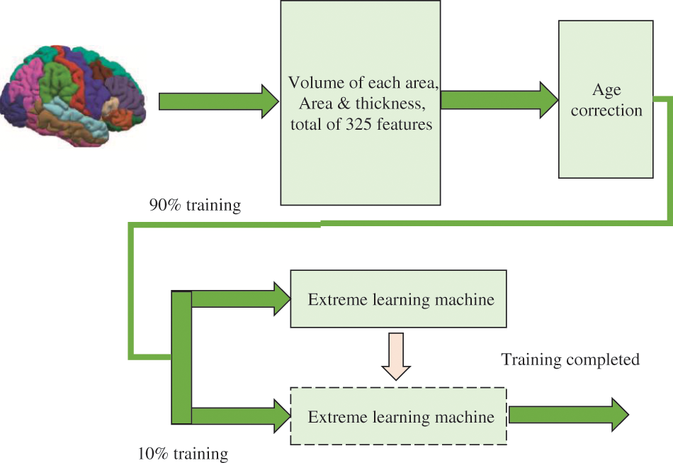
Figure 2: Proposed framework

2.1 Dataset

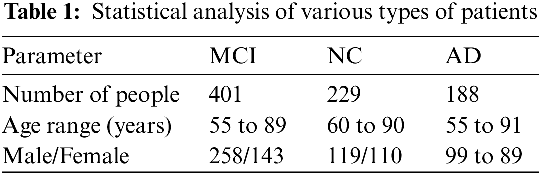
The ADNI is an international public database of AD research. In 2004, it invested 67 million US dollars to recruit more than 800 volunteers for long-term follow-up [23], collected and analyzed thousands of brain images, gene maps, blood and blood samples. The purpose of biomarkers in spinal fluid is to study the pathogenesis of the disease and find effective treatments, and these data have been made public to researchers around the world. In 2011, the ADNI invested another $67 million to conduct a new round of volunteer recruitment and data collection, called ADNI2. At present, the work of ADNI2 has been completed, and the third phase of the project, ADNI3, is in progress. This study used the magnetic resonance data of some test subjects in the ADNI1 standard database for experiments, including 188 patients, 229 normal people and 401 mild cognitive impairment patients, a total of 818 patients, and their statistical data are shown in Table 1.

FreeSurfer is a free magnetic resonance data processing software package jointly developed by Harvard-MIT Department of Health Sciences and Technology and Massachusetts General Hospital [24], which can perform automatic cortical and subcutaneous nuclei segmentation, as shown in Fig. 3. In this study, the 4.3 version of the software was used to analyze the magnetic resonance images of the above objects to obtain anatomical features. These features were obtained by FreeSurfer’s automatic segmentation of various regions of the cerebral cortex, including the volume of each region. There are 325 features in total, such as surface area, average thickness and standard deviation of thickness. These characteristic values can be downloaded directly from the ADNI website (http://adni.loni.usc.edu/).

Figure 3: Brain illustration via FreeSurfer

2.2 Age Correction

Some literatures have pointed out that with normal aging, some areas of the brain will naturally atrophy [25], and with the increase of age, the cerebral gray matter volume and age show a linear relationship with a negative slope. This shrinking phenomenon is similar to brain shrinkage in AD. Therefore, in the test subjects of different ages, the atrophy of their brains is not entirely caused by AD, but also partly due to natural atrophy caused by aging.

In order to reduce the confounding of age-related atrophy, this study reduces the error caused by normal aging factors by estimating the effect of normal aging on brain atrophy [26], and offsetting this effect from the aforementioned anatomical features of the brain. The suggested method for diagnosing AD simply makes use of readily available and inexpensive MRI data.

In order to estimate the atrophy effect of normal aging, first select the characteristic data of N normal people, and form the values of all normal subjects of the mth characteristic into a vector [y1m,…,ynm,…,yNm]T, and then perform linear regression fitting to obtain the straight line y=ax+b, where a, b are real numbers. The linear relationship between a certain feature and age can be obtained from this model, that is, the changing trend of a certain feature with age can be known from the coefficient a.

By doing the same operation on all the features of the MRI brain image, the relationship between all the features and age can be estimated. The age of all subjects is composed of age matrix X, the characteristics of all normal people are composed of feature matrix Y, and the coefficient matrix β is set. They are expressed in Eqs. (1) to (3) as follows:

X=[x1x2⋮xN 11⋮1](1)

β=[a1b1 a2b2 ⋯⋯ aMbM](2)

Y=[y11y21⋮yN1 y12y22⋮yN2 ⋯⋯⋯⋯ y1My2My3MyNM](3)

In the formula, N is the number of normal subjects, and M is the number of characteristic values.

Then, linear regression fitting is performed, and the fitting goal is to establish a linear regression model, that is expressed in Eq. (4):

Y=Xβ+ε(4)

In the formula, ε is the fitting error, Y is the feature matrix, and β is the coefficient matrix. According to the principle of least squares linear fitting, to make ∑ε2 the smallest, the solution of the optimal coefficient matrix β is expressed in Eq. (5):

β=(XTX )−1XTY(5)

After obtaining β, the linear relationship a1,a2,…,aM between all features and age can be obtained from it. Then, according to this relationship, use the following formula to remove the age factor in the characteristics of all experimental subjects, and calculate a new characteristic value fnew,nm, where fnm represents the mth characteristic of the nth subject, and it is expressed in Eq. (6):

fnew,nm=fnm−amxn(6)

2.3 Extreme Learning Machine

After age correction as described above, the characteristics of all subjects were used for the computer diagnosis of AD. The extreme learning machine is used as a classifier to distinguish different object category groups [27]. It is a single hidden layer neural network that can be used for classification, regression and clustering purposes. Different from other traditional neural networks that use error backpropagation, it first generates and fixes the input layer coefficients, and directly calculates the output layer coefficients according to the input and output values of the training data during the training process. Its advantage is that the training speed is fast, and its classification effect is better than that of the usual support vector machine [28].

The principle of extreme learning machine is shown in Fig. 4, where the neural network has only one hidden layer. The variable x represents the feature vector of an input sample, and the output of the ith node in the hidden layer is hi(x)=G(ai,bi,x), where ai and bi are the input layer coefficients, and G(x) is the mapping functions, such as G(ai,bi,x)=sigmoid(aiTx+bi). The output of the L nodes in the hidden layer is formed into a vector h(x)=[h1(x),…,hL(x)]. The result of the extreme learning machine output is f(x)=h(x)β, where β=[β1,β2,…,βL]T is the output layer coefficient.

Figure 4: Extreme learning machine architecture [28]

The training process of extreme learning machine can be divided into the following three steps:

Step 1: Randomly generate input layer coefficients ai and bi.

Step 2: Calculate the hidden layer output matrix H=[h(x1),h(x2),…,h(xN)]T, where N represents the number of training samples.

Step 3: Assuming that y is the classification label vector corresponding to the N samples, the optimal solution for calculating the output layer coefficient β should satisfy the constraint of Eq. (7):

minβ⁡||y−HB||2(7)

The optimal solution for computing β can be obtained by computing β=H+y, where H+ is the Moore-Penrose generalized inverse of the H matrix.

When the training is over, the input layer coefficients ai and bi and the output layer coefficient β of the neural network have been determined, then the extreme learning machine can classify the test data. However, because the input layer coefficients ai and bi are randomly generated, the effect is not good. The improved version of the extreme learning machine adopts the kernel function mapping method similar to the support vector machine. In the way of using the kernel function, the output vector h(x) of the hidden layer does not need to be calculated, thus avoiding the randomness of the coefficients of the input layer. The relationship between the output and input of the extreme learning machine can be expressed as in Eq. (8):

f(x)=[K(x,x1)⋮K(x,xn)⋮K(x,xN)][1C+Ω]−1y(8)

where K(u,v) represents the kernel function, C is the normalization coefficient, xn represents the eigenvector of the nth sample, x represents the eigenvector of the tested sample, and Ω represents the N×N kernel matrix, where each element of can be expressed as Ωij=h(xi).h(xj)=K(xi,xj), when the kernel function is determined, h(xi).h(xj) does not need to be calculated, and K(xi,xj) can be calculated.

3  Simulation Results

3.1 Simulation Configuration

In this section, the experimental configuration is mentioned. A total of 818 participants had their anatomical characteristics calculated using the FreeSurfer programme utilizing information from the ADNI dataset. After being preprocessed with an age correction approach that uses linear regression to assess the effects of natural ageing, these attributes were initially taken out of the dataset.

3.2 Estimated Results for Age Factors

In the process of age correction, linear fitting was performed using the characteristics of all normal subjects in the dataset (the number of people was 229). The fitting of some features is shown in Fig. 5, where the dots represent the characteristic values of each experimental object, and the straight lines represent the fitting results. It can be seen that the volume and thickness have a downward trend with age, which is also in line with the conclusion that normal aging will atrophy the brain tissue.

Figure 5: Comparison of estimated linear regression. (a) Volume; (b) thickness

3.3 Comparison of Diagnostic Test Results

In order to test the effect of the proposed method in the automatic diagnosis of AD, 818 subjects in ADNI1 were used as samples, and each subject had 325 age-corrected characteristics. All subjects were divided into three groups: patients, mild cognitive impairment and normal people. In the experiment, patients and normal people with MCI, and normal people and three groups were tested for three categories at the same time. The test plan uses the ten-fold cross-validation method to conduct the experiment, that is, all the test objects are divided into 10 equally, 9 of which are used for training the extreme learning machine, and the remaining 1 is used for testing and diagnosis. It is used for 1 test, and finally the results of all object tests are obtained. In order to ensure the robustness of the experiment, the above ten-fold cross-validation process was repeated 100 times. Each time the order of the objects was randomly scrambled, they were randomly divided into 10 parts, and the average and standard deviation of the results of the last 100 times were taken as the final result.

The test results were counted as accuracy (ACC), specificity (SPE), sensitivity (SEN) and area under the curve (AUC). Among them, the accuracy rate represents the probability that the test sample category is correctly estimated, the specificity represents the probability that the negative sample is accurately estimated to be negative, and the sensitivity represents the probability that the positive sample is accurately estimated to be positive. The area under the curve is the area under the receiver operating characteristic (ROC) curve, and its maximum value is 100%, which is often used to evaluate the superiority of binary classifiers, as shown in Fig. 6. The experiment was carried out in MATLAB 2014a software, and the test computer platform configuration: CPU was i5 7400, RAM was 8 GB, and the operating system was Windows 10. The test results are shown in Tables 2–4.

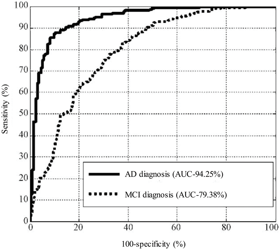
Figure 6: Comparison of the sensitivity of MCI and AD

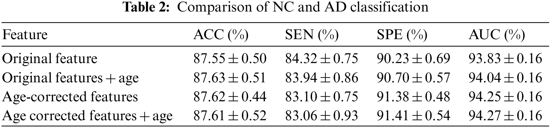
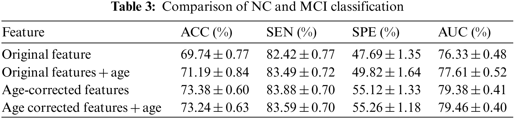
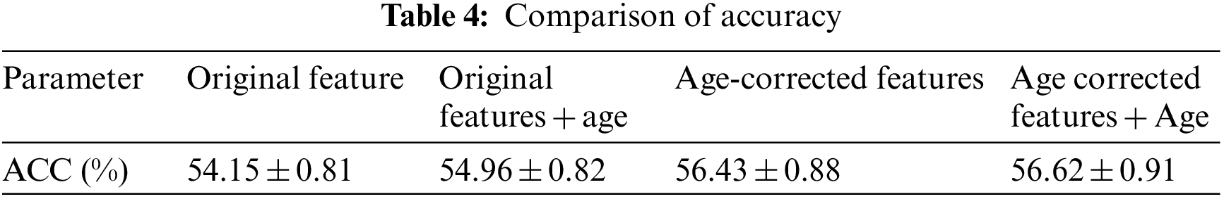
It can be seen from the above experimental results that the proposed method can achieve an accuracy rate of 87.62% for the diagnosis between patients and normal people, and the area under the curve reaches 94.25%, indicating that the proposed method is effective in AD. It has excellent performance in classification and diagnosis. The standard deviation of the 100-time verification of the diagnostic accuracy was only 0.44%, indicating that the results of the method were relatively stable and robust. It can also reach 73.38% for mild cognitive impairment that is difficult to diagnose, and its sensitivity reaches 83.88%, indicating that it can better detect the MCI. For the results of the three-category diagnosis, the accuracy rate is only 56.43%, indicating that there is still room for improvement. It can be seen from Table 2 that age correction has little effect on the diagnosis of AD, only the area under the curve increases slightly. However, from Table 3, it can be found that age correction has a greater improvement in the accuracy of diagnosing MCI, and if age is directly added as a feature to the original feature, although the performance has a certain improvement effect, the effect than age correction. After age correction, adding age as a feature has no effect. The age correction also has a certain improvement effect on the accuracy of the three classifications.

3.4 Comparison with Other Methods

In order to compare the effect of extreme learning machine and other classifiers, this study also tested two classifiers, support vector machine and random forest, in which support vector machine uses MATLAB’s own functions svmtrain and svmclassify, while random forest uses a third-party library. The results of the comparison are shown in Table 5. It can be found that in the diagnosis of AD and MCI, the classification method of extreme learning machine has the highest accuracy among the three classifiers, and the classification effect of random forest is slightly worse than that of extreme learning machine. The accuracy rate is higher than that of the support vector machine classifier. Table 5 also compares two other types of methods, such as the method using the volume of the ROI as a feature, using a support vector machine as a classifier, and extracting features from the hippocampus and posterior cingulate cortical regions, using principal components analysis and support vector machine as a classifier method. Compared with these two methods, the proposed method has higher accuracy.

4  Discussion

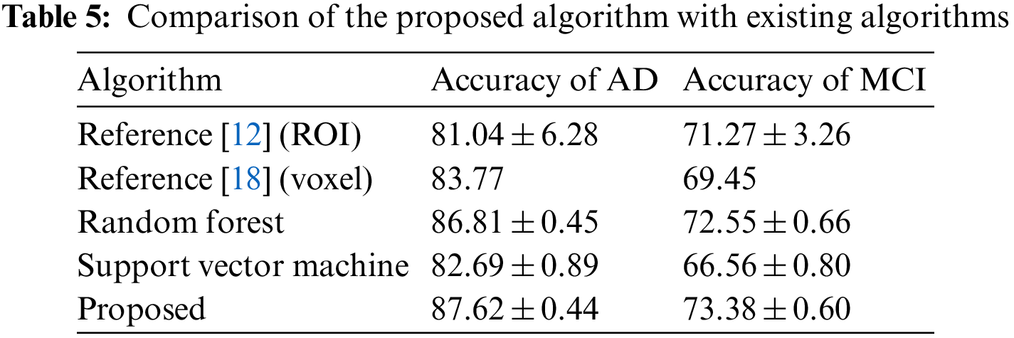
Currently, the commonly used diagnostic methods for AD are based on the scores of clinical intelligence test scales, such as the Mini-Mental State Examination Scale, the Clinical Dementia Rating Scale, the Functional Activity Questionnaire, and the Alzheimer’s Disease Rating Scale. However, these tests are subject to subjective and random factors that affect the diagnosis of the disease, with greater error in the diagnosis of mild cognitive impairment. The diagnosis method based on MRI image has the advantages of being objective and reliable, which helps to improve the accuracy of diagnosis. Compared with methods that use MRI image ROI volume or image voxel value as features, the whole brain anatomical features calculated from MRI images can more comprehensively reflect the brain atrophy pattern caused by AD. It can be seen from the experimental results that based on the anatomical characteristics of MRI, the age correction combined with the extreme learning machine diagnosis method in this study has a higher accuracy than the method of using support vector machine to diagnose MRI images. In the diagnosis of MCI, the proposed method also has good accuracy and high sensitivity. Sensitivity represents the probability that a real patient is diagnosed as a patient, and a high sensitivity indicates that the method has a low rate of missed diagnosis, that is, it can efficiently detect patients with mild cognitive impairment from normal people. Since there is currently no drug to treat AD, early detection of people with mild cognitive impairment is key. The proposed research method is of great significance for the high sensitivity of the diagnosis of MCI. It helps therapists to detect patients in time and implement intervention measures as soon as possible to reduce the probability of mild cognitive impairment developing into AD or delay the onset of the disease.

The authors used MRI image features to diagnose mild cognitive impairment, and the accuracy rates were 71.27% and 69.45%, respectively. The anatomical features of MRI and the diagnostic performance of features plus age were similar. However, after processing the original features by the age correction algorithm in this study, the diagnostic accuracy was again improved to 73.38%, which is higher than the methods, indicating that the age correction algorithm is indeed helpful to improve the diagnostic accuracy of MCI. From the experimental results in Table 2, this method is less helpful for the diagnosis of AD, while the results in Table 3 show that this method has a greater effect on the diagnosis of MCI. The reason may be that: AD patients have more severe atrophy, and the proportion of atrophy caused by age factors is smaller, while those with MCI have less atrophy, and the proportion of atrophy caused by corresponding age factors is higher. Therefore, excluding the age factor in the diagnosis of MCI can greatly improve its accuracy. The results also indicate that in the diagnosis of MCI, the interference factors caused by normal aging will have a greater impact on the diagnosis results, and reasonable methods should be used to offset or reduce the interference.

It is more practical to classify patients, MCI and normal people into three categories, but its classification is also more difficult. Some studies have compared the results of 29 algorithms on three-classification [29], only one algorithm has an accuracy rate of more than 60%, and the accuracy of some algorithms is close to a random classifier, which shows the difficulty of three-classification. In this method, the original features were first used for three classifications, and the accuracy of diagnosis was only 54.15%, and the accuracy of three classifications was increased to 56.43% after adding age correction. Although the accuracy rate is not high, the practice of using age correction to improve the accuracy of three-category diagnosis has certain reference value [30].

The proposed method for diagnosing AD only uses MRI data that is relatively inexpensive and easy to obtain. To improve the accuracy of diagnosis, multimodal data fusion can be used to combine the useful features of various medical images. Although the diagnostic accuracy was only 81.04% when only MRI was used, after the fusion of positron emission tomography data and MRI data, the accuracy was increased to 91.4%. Therefore, the use of multimodal data fusion to improve the diagnostic accuracy is the future research direction of the author.

5  Conclusion

This study proposes a computer-based automatic diagnosis method for AD based on the anatomical features of structural magnetic resonance brain images. Through the training of age-corrected and extreme learning machine classifiers, and verified on the data of ADNI database, the accuracy of diagnosing AD can reach 87.57%, and the diagnosis of MCI can reach 73.38%, the sensitivity reached 83.88%, which is of great significance for early detection and prevention of AD. The accuracy of the proposed method in three-classification needs to be improved, and using multimodal input to improve the accuracy of three-classification will be the direction of improvement in future research.

The suggested approach for diagnosing AD simply makes use of MRI data, which is accessible and reasonably priced. Multimodal data fusion can be used to integrate the beneficial elements of diverse medical pictures to increase the accuracy of diagnosis. When using simply MRI, the diagnosis accuracy was only 81.04%; however, after combining MRI and positron emission tomography data, the accuracy was enhanced to 91.4%. Therefore, the author’s intended future research focus is on using multimodal data fusion to increase diagnostic precision.

Funding Statement: The authors received no specific funding for this study.

Availability of Data and Materials: The data used for the findings of this study is available upon request from the corresponding author.

Conflicts of Interest: The authors declare that they have no conflicts of interest to report regarding the present study.

References

1. S. Shoukry, T. Rassem and N. Makbol, “Alzheimer’s diseases detection by using deep learning algorithms: A mini-review,” IEEE Access, vol. 8, pp. 77131–77141, 2020. [Google Scholar]

2. T. Vos, C. Allen and M. Arora, “Global, regional, and national incidence, prevalence, and years lived with disability for 310 diseases and injuries, 1990–2015; a systematic analysis for the global burden of disease study 2015,” Lancet, vol. 386, no. 10053, pp. 1545–1602, 2016. [Google Scholar]

3. X. Du, W. Chao and Q. Liu, “Potentials roles of selenium and selenoproteins in the prevention of Alzheimer’s disease,” Current Topics in Medicinal Chemistry, vol. 16, no. 8, pp. 835–848, 2016. [Google Scholar] [PubMed]

4. W. Khan, E. Westman, N. Jones, L. Wahlund, P. Mecocci et al., “Automated hippocampal subfield measures as predictors of conversion from mild cognitive impairment to Alzheimer’s disease in two independent cohorts,” Brain Topography, vol. 28, pp. 746–759, 2015. [Google Scholar] [PubMed]

5. L. Pini, M. Pievani and M. Bocchetta, “Brain atrophy in Alzheimer’s disease and aging,” Ageing Research Reviews, vol. 30, no. 5, pp. 25–48, 2016. [Google Scholar] [PubMed]

6. E. Moradi, A. Pepe and C. Gaser, “Machine learning framework for early MRI-based Alzheimer’s conversion prediction in MCI subjects,” Neuroimage, vol. 104, no. 3, pp. 398–412, 2015. [Google Scholar] [PubMed]

7. C. Moller, P. Ya and V. Wm, “Alzheimer disease and behavioral variant frontotemporal dementia: Automatic classification based on cortical atrophy for single-subject diagnosis,” Radiology, vol. 279, no. 3, pp. 838–848, 2016. [Google Scholar] [PubMed]

8. C. Cabral, P. Morgado and C. Campos, “Predicting conversion from MCI to AD with FDG-PET brain images at different prodromal stages,” Computers in Biology & Medicine, vol. 58, pp. 101–109, 2015. [Google Scholar]

9. K. Gray, R. Wolz and R. Heckemann, “Multi-region analysis of longitudinal FDG-PET for the classification of Alzheimer’s disease,” Neuroimage, vol. 60, no. 1, pp. 221–229, 2012. [Google Scholar] [PubMed]

10. T. Nir, J. Villalong and G. Prasad, “Diffusion weighted image-based maximum density path analysis and classification of Alzheimer’s disease,” Neurobiology of Aging, vol. 36, no. 3, pp. 132–140, 2015. [Google Scholar]

11. P. Selnes, D. Aarsland and A. Bjornerud, “Diffusion tensor imaging surpasses cerebrospinal fluid as predictor of cognitive decline and medical temporal lobe atrophy in subjective cognitive impairment and mild cognitive impairment,” Journal of Alzheimer’s Disease, vol. 33, no. 3, pp. 723–736, 2013. [Google Scholar] [PubMed]

12. S. Liu, S. Sidong and W. Cai, “Multi-modal neuroimaging feature learning for multi-class diagnosis of Alzheimer’s disease,” IEEE Transactions on Biomedical Engineering, vol. 62, no. 4, pp. 1132–1140, 2015. [Google Scholar] [PubMed]

13. T. Tong, K. Gray and Q. Gao, “Multi-modal classification of Alzheimer’s disease using nonlinear graph fusion,” Pattern Recognition, vol. 63, no. 3, pp. 171–181, 2017. [Google Scholar]

14. S. Rathore, M. Habes and M. Aksam, “A review on neuroimaging-based classification studies and associated feature extraction methods for Alzheimer’s disease and its prodromal stages,” Neuroimage, vol. 155, no. 3, pp. 530–548, 2017. [Google Scholar] [PubMed]

15. H. Jia, Y. Wang, Y. Duan and H. Xiao, “Alzheimer’s disease classification based on image transformation and features fusion,” Computational and Mathematical Methods in Medicine, vol. 2021, pp. 1–10, 2021. [Google Scholar]

16. K. Wei, W. Kong and S. Wang, “An improved multi-task sparse canonical correlation analysis of imaging genetics for detecting biomarkers of Alzheimer’s disease,” IEEE Access, vol. 9, pp. 30528–30538, 2021. [Google Scholar]

17. R. Cuingnet, E. Gerardin and J. Tessieras, “Automatic classification of patients with Alzheimer’s disease from structural MRI: A comparison of ten methods using the ADNI database,” Neuroimage, vol. 56, no. 2, pp. 766–781, 2011. [Google Scholar] [PubMed]

18. A. Ben, M. Mizotin and J. Benois, “Alzheimer’s disease diagnosis on structural MR images using circular harmonic functions descriptors on hippocampus and posterior cingulate cortex,” Computational Medical & Graphics, vol. 44, pp. 13–25, 2015. [Google Scholar]

19. J. Sheng, Y. Xin, Q. Zhang, L. Wang, Z. Yang et al., “Predictive classification of Alzheimer’s disease using brain imaging and genetic data,” Scientific Reports, vol. 12, no. 3, pp. 1–9, 2022. [Google Scholar]

20. Z. Fan, F. Xu, C. Li and L. Yao, “Application of KPCA and AdaBoost algorithm in classification of functional magnetic resonance imaging of Alzheimer’s disease,” Neural Computing and Applications, vol. 32, no. 5, pp. 5329–5338, 2020. [Google Scholar]

21. R. Jain, N. Jain, A. Aggarwal and D. Hemanth, “Convolutional neural network based Alzheimer’s disease classification from magnetic resonance brain images,” Cognitive Systems Research, vol. 57, no. 3, pp. 147–159, 2019. [Google Scholar]

22. F. Zhang, Z. Li and B. Zhang, “Multi-modal deep learning model for auxiliary diagnosis of Alzheimer’s disease,” Neurocomputing, vol. 361, no. 1, pp. 185–195, 2019. [Google Scholar]

23. B. Wyman, D. Harvey and K. Crawford, “Standardization of analysis sets for reporting results from ADNI MRI data,” Journal of the Alzheimer’s Association, vol. 9, no. 3, pp. 332–337, 2013. [Google Scholar]

24. B. Fischl and A. Dale, “Measuring the thickness of the human cerebral cortex from magnetic resonance images,” National Academy of Sciences, vol. 97, no. 20, pp. 11050–11055, 2000. [Google Scholar]

25. A. Giorgio, L. Santelli and V. Tomassini, “Age-related changes in grey and white matter structure throughout adulthood,” Neuroimage, vol. 51, no. 3, pp. 943–951, 2010. [Google Scholar] [PubMed]

26. J. Dukart, M. Schroeter and K. Mueller, “Age correction in dementia-matching to a healthy brain,” PLoS One, vol. 6, no. 7, pp. 1018–1029, 2011. [Google Scholar]

27. J. Kim and B. Lee, “Automated discrimination of dementia spectrum disorders using extreme learning machine and structural T1 MRI features,” in IEEE Int. Conf. on Engineering in Medicine and Biological Society, Jeju, South Korea, pp. 1990–1993, 2017. [Google Scholar]

28. G. Huang, H. Zhou and X. Ding, “Extreme learning machine for regression and multiclass classification,” IEEE Transactions on Systems Man & Cybernetics Part B, vol. 42, no. 2, pp. 513–529, 2012. [Google Scholar]

29. E. Bron, M. Smits and V. Wm, “Standardized evaluation of algorithms for computer-aided diagnosis of dementia based on structural MRI: The CAD dementia challenge,” Neuroimage, vol. 111, no. 3, pp. 562–579, 2015. [Google Scholar] [PubMed]

30. A. Kumar, “Study and analysis of different segmentation methods for brain tumor MRI application,” Multimedia Tools and Applications, vol. 8, no. 2, pp. 1–23, 2022. [Google Scholar]