Prediction-Based Thunderstorm Path Recovery Method Using CNN-BiLSTM

1  Introduction

Thunderstorm-induced severe weather changes are very likely to develop into meteorological disasters. With the rapid development and application of modern microelectronic devices and information technology, ever greater importance is attracted to thunderstorm disaster precautions and preventions [1,2]. In recent years, thunderstorm data acquisition channels have been greatly expanded over traditional manual observations. An atmospheric electric field (AEF) near the ground is directly related to the charges carried by thunderstorm clouds. AEF apparatus (AEFA) used to measure AEFs is suitable for detecting short-range thunderstorm activities, with a better application prospect in small-scale regional thunderstorm warning [3–5].

The traditional AEF-based thunderstorm warning methods mainly include AEF threshold, polarity reversal, and fast-change jitter methods. The related researches involve algorithms such as principal component analysis, clustering, and region identification. However, they generally suffer from low warning rates and greater difficulties in visualizing thunderstorms [6–9]. These problems mainly stem from their dependence on a single vertical AEF. In fact, the charge center of a thunderstorm cloud is not always directly above AEFA, and the AEF generated at the observation station has some non-negligible horizontal components. In other words, three-dimensional AEF (3DAEF) consisting of horizontal and vertical components exists theoretically [5,7,10]. Improvements in 3DAEF measurement methods and its matching apparatuses quickly overcome reliance on traditional methods [11–14]. For example, Xing et al. [11] establishes a 3DAEF measurement model and proposes a thunderstorm cloud point charge localization method. The effectiveness of their method is verified by the performance analyses of ranging and direction finding and actual experiments. Reference [12] develops a high-altitude 3DAEF apparatus (3DAEFA), consisting of three orthogonal induction sheets with specially designed insulation and battery cells. A hybrid 3DAEFA is also designed to measure 3DAEFs on the ground in [13]. In a thunderstorm activity observation, the thunderstorm-intensive area position is successfully pointed out. Meanwhile, this position basically matches the one given by the lightning locator.

With the rise of artificial intelligence (AI) technology, the practical 3DAEF-based thunderstorm detection works have witnessed impressive progress in recent years [14–17]. In [14], an entropy-distribution based AEFS division provides temporal information for cluster-based spatial point charge denoising. Most importantly, the formation of AEF signal (AEFS) prediction framework is promoted with its combination of the convolutional neural network (CNN), long short-term memory (LSTM), and bi-directional LSTM (BiLSTM). Considering the adoption of data-driven AI algorithms to solve real-time forecasting of extreme weather events, a deep learning method is proposed in [15] that takes videos of radar reflectivity frames as the input for timely thunderstorm prediction. The prediction performance is assessed by converting the resulting probabilistic results into binary classifications. Reference [16] takes into account of AEFS’s oscillatory scale properties. An ensemble empirical mode decomposition first decomposes AEFS to generate multiple components. Further, an extreme gradient boosting (XGBoost) model is utilized to fuse the extracted component features for a final thunderstorm warning. Reference [17] predicts the thunderstorm occurrences with nonlinear models. Specifically, a Jacobi algorithm is used to construct a prediction model with six inputs and one output, achieving an impressive estimation error of 5.73%. Yet, prediction errors are unfortunately found to be high during the monsoon season. On the whole, these works entail a basic assumption that each 3DAEFA in the field works properly. But poor environmental stability makes it difficult to guarantee in most detection scenarios. Therefore, a solution to AEF data loss would have greater practical significance for thunderstorm protection and disaster reduction.

Currently existing data recovery efforts mainly focus on predictions using neural networks. LSTM has been proposed to predict AEFs for its ability to learn long-term dependencies between time-step sequence data [5,18]. Especially, considering the strong spatiotemporal correlation of AEFS, LSTM is combined with BiLSTM [14]. In addition, the clustering algorithms such as improved fuzzy C-means are adopted to divide AEF samples and extract fuzzy rules to overcome prediction model complexities, namely, low accuracy and short prediction time due to complex thunderstorm data and larger input dimensions [19,20]. But to the best of our knowledge, there is no recovery to thunderstorm point charge movement paths based on lost AEF data in existing works. At the same time, weather conditions corresponding to AEF are directly related to the recovery implementation necessity.

This paper focuses on AI-based AEF prediction and weather judgment model establishment corresponding to different AEFs. Based on currently available works, it pays more attention to AEF-based thunderstorm path visualization and prediction validity. In particular, according to a spatial orientation relationship between a point charge and a 3DAEFA, the implementation steps of point charge localization and its moving path fittings are presented. Performance comparisons against radar charts and existing works are made to compare the proposed method with other methods. In this way, this work proposes a real-time monitoring scheme of thunderstorm activities under AEF data loss.

Major contributions of this paper are the following.

1)   The proposal of a novel thunderstorm path recovery method.

2)   3DAEF-based thunderstorm point charge path acquisition.

3)   Defining recovery rules based on predicted value intervals.

This paper is organized as follows. Section 2 elaborates on thunderstorm paths. Section 3 describes the path recovery process. Section 4 evaluates the performance of the proposed method. Section 5 discusses experiment results, followed by conclusions in Section 6.

2  Thunderstorm Path

This section firstly establishes a localization model for thunderstorm point charges, and then deduces localization formulae according to relative position relationships between a point charge and a 3DAEFA. According to the original AEF time series, a curve fitting is carried out on localization results to obtain point charge movement paths in space domains. Following that, the design principle, structure and calibration of the core apparatus 3DAEFA are described in detail.

2.1 Localization Model

To determine the relationships between 3DAEF components and point charge positions, a model for point charge localization is established, as shown in Fig. 1 [5,11,14].

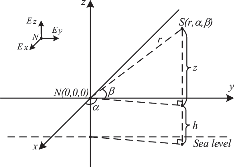
Figure 1: A localization model for thunderstorm point charges

In Fig. 1, a 3D coordinate system is established with a 3DAEFA point N(0,0,0) as the origin. The positive half-axis of the coordinate system x-axis and y-axis are defined as north and east respectively. h represents the sum of 3DAEFA height and its locational elevation. r is the distance from point charge S to N. The horizontal and elevation angles of S are α and β respectively. S(x,y,z) and S(r,α,β) are rectangular and spherical coordinates of charge S, respectively.

Based on the mirror method theory [7,21], it is assumed that the thunderstorm cloud is a point charge q. The potential distribution φ of charge q at apparatus N is

φ=14πε1(qx2+y2+(z−h)2−ε2−ε1ε2+ε1q′x2+y2+(z+h)2)(1)

where q′ is the image charge of point charge q. ε1 and ε2 respectively represent the permittivities of the  air and the ground where 3DAEFA is located.

By taking derivatives of φ in the direction of x, y and z axes, we obtain

{Ex=∂φ∂x=−qx4πε1{[x2+y2+(z−h)2]−32−ε2−ε1ε2+ε1[x2+y2+(z+h)2]−32}Ey=∂φ∂y=−qy4πε1{[x2+y2+(z−h)2]−32−ε2−ε1ε2+ε1[x2+y2+(z+h)2]−32}Ez=∂φ∂z=−q4πε1{(z−h)[x2+y2+(z−h)2]−32−ε2−ε1ε2+ε1(z+h)[x2+y2+(z+h)2]−32}(2)

where Ex, Ey and Ez are AEF intensities of charge q in x-, y- and z-axis directions collected with 3DAEFA, respectively.

Usually, we have [5,11,14]

{z≈z−h≈z+hr=x2+y2+z2(3)

After substituting Eq. (3) into Eq. (2), we get

{r=A2(1−B)2Ex2+Ey2+Ez24α={arctanEyEx,when Ex>0arctanEyEx+180∘,when Ex<0 and Ey>0arctanEyEx−180∘,when Ex<0 and Ey<0β=arctanε1|Ez|ε2Ex2+Ey2(4)

In Eq. (4), A=−q4πε1 and B=ε2−ε1ε2+ε1. Here, once 3DAEF components Ex, Ey and Ez are acquired, the localization results are obtained using Eq. (4).

2.2 Point Charge Path

The development from a single vertical AEF component to 3DAEF provides an essential data source for thunderstorm localization. In this paper, a self-made 3DAEFA [14] is used for 3DAEF data acquisition. Theoretically, 3600 time series 3DAEF data are collected per hour, based on a sampling frequency of 1 Hz. An operation with Eq. (4) obtains localization results concerning time series in thunderstorm point charges. A mere analysis to a large number of localization results only roughly estimates and judges the thunderstorm activity and movement trajectory from perspectives, such as charge accumulation, charge development, distances from accumulated charges to 3DAEFA, and changes in the height and elevation angle of charges. It is inadequate to observe a thunderstorm movement intuitively and clearly. On this account, the point charge coordinate data of a certain plane (X0Y, X0Z and Y0Z) are adopted for curve fitting, with the help of the polynomial function in CFtool toolbox. Under the premise to ensure the inherent timing of charge positions, a polynomial fitting is performed on localization results to obtain point charge paths. The curve here is defined as the imaged moving path of point charges obtained from this fitting. This effectively improves and strengthens thunderstorm visualizations.

2.3 3DAEFA Details

Fig. 2 presents a designed single-axis rotary vane 3DAEF sensor fixed on 3DAEFA for real-time 3DAEF acquisition.

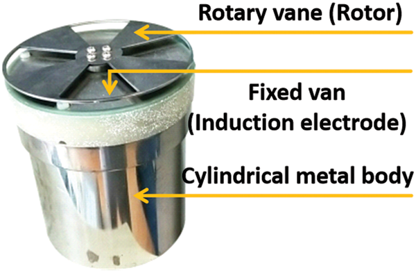
Figure 2: The physical picture of 3DAEF sensor

2.3.1 Principle

Based on the electrostatic induction theory [14,22], the free electrons move inside the metallic body in the electrostatic field, under AEF actions. Positive and negative charges (PCs and NCs) move along and against AEF directions, respectively, so that these two kinds of charges are separated. PCs leave the metal and then flow into the earth through the operational amplifier (OA) to generate a pulse current. This current is then converted into the voltage signal output, after the current-to-voltage transformation.

Such a pulse signal causes the current to be generated only once. Therefore, these charges require continuous induction to obtain steady current signals. In other words, it is necessary to periodically expose the metal electrode to AEF. PCs are repelled away, resulting in a positive current, when the electrode is exposed to AEF. Remaining NCs flow through OA to form a negative current, when the electrode is shielded. The cycle between exposure and shielding ensures a steady alternating current generation. Induced charges are proportional to AEF intensity, so the output voltage signal proportional to that intensity is acquired after a series of processing.

2.3.2 Structure

Fig. 3 illustrates the internal cylindrical 3DAEF sensor’s components. The cylinder’s outer layer is a shielded electrode, whose upper surface and side are hollow cylindrical metal sheets. The hollow shape with a 1:1 hollow ratio matches the distribution of induction electrodes. To avoid the vibration or deformation during the rotation, the shielded electrode has fixed one ring at the upper surface edge and another one at the side bottom edge. Induction electrodes X, Y, Z and the rotary vane are respectively made of copper and stainless steel.

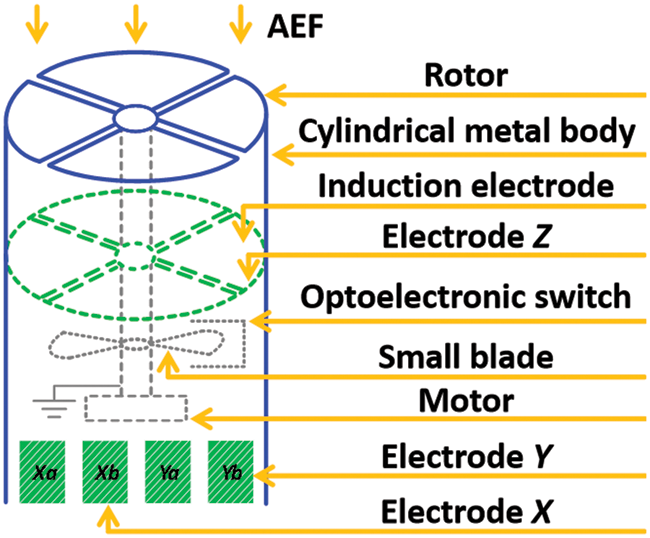
Figure 3: The internal structure of 3DAEF sensor

2.3.3 Calibration

The vertical AEF Ez is calibrated by adjusting the calibration equipment output and external electric field (EEF) until both values are consistent, based on a one-dimensional (1D) AEF calibration method proposed in [22,23]. Fig. 4 presents the horizontal AEF intensity (Ex and Ey) calibration. A standard EEF Es with known intensities is generated by applying voltages.

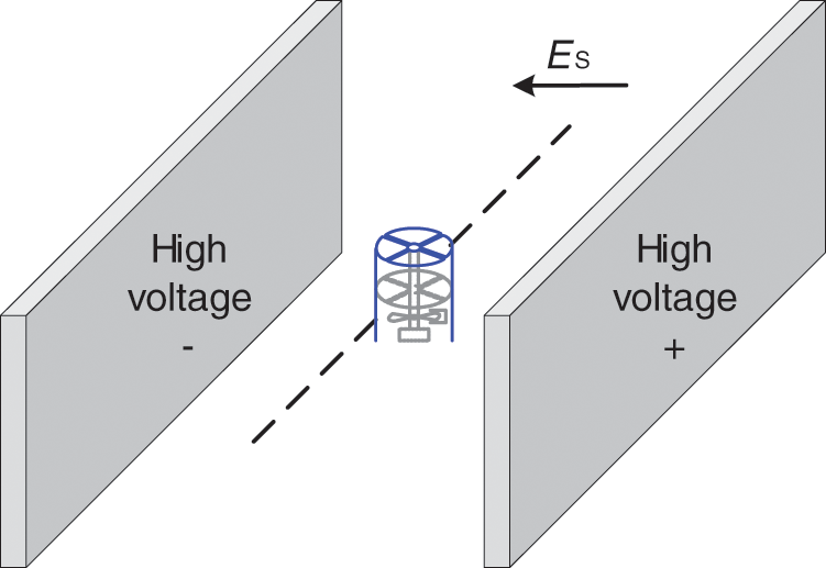
Figure 4: The schematic of horizontal AEF intensity calibration

3DAEF sensor is firstly placed between the vertical pair of parallel plates. Induction electrodes in X-direction are placed in the same direction as EEF direction. Ex calibration is accomplished by adjusting parameters so that X-direction signal output is consistent with that of EEF. The sensor is rotated 90∘ so that induction electrodes in Y-direction are consistent with that of EEF direction. Ey calibration is finally accomplished by adjusting parameters so that Y-direction output is consistent with that of EEF.

3  Thunderstorm Path Recovery

AEF data loss is inevitable. This section first uses an AI-based model combining CNN and BiLSTM [14,24] to predict lost AEF. Meanwhile, an XGBoost model combined with stacked autoencoder (SAE) [16,25,26] is introduced to define path recovery rules for different AEF-based weather conditions.

3.1 AEF Data Recovery

Fig. 5 illustrates an established CNN-BiLSTM model for AEF data recovery.

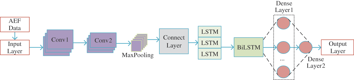
Figure 5: A CNN-BiLSTM model for AEF data recovery

In Fig. 5, it takes AEF data without losses as the input to the model. The proposed model mainly has two blocks. Specifically, there are two 1D CNN layers (Conv1 and Conv2) with 256 and 128 filters, respectively, in the first block. A hybrid layer composed of three LSTM layers and one BiLSTM layer is included in the second block. LSTM and BiLSTM layers have 100 and 128 units respectively. Following these two blocks, the dense layer outputs AEF prediction results. The learning rate and epochs are set to 0.0001 and 10, respectively. The data input of the model is set to 6000 (i.e., 100 min), and the ratio of training set and test set is set to 7:3. Note that Adam is used as the optimizer.

Since there are no thunderstorms in sunny weather, there are certainly no paths. Here, the output of CNN-BiLSTM model (that is, the recovered AEF with 1800 samples) is used as the input of SAE-XGBoost model to judge weather conditions of the recovered AEF. Finally, the weather decides whether it is necessary to fit the paths.

3.2 SAE-XGBoost Model

Fig. 6 presents AI-based AEF testing flow based on a SAE-XGBoost model, including training and testing parts.

1)   Training part: To better mine time-domain features of AEF data and adapt SAE model, the selected sunny and thunderstorm weather’s AEF data are first normalized, and a two-layer SAE is constructed for feature extractions. After labeling sunny and thunderstorm AEF data with 0 and 1 respectively, these data are input into XGBoost network for training. In particular, the genetic algorithm (GA) is adopted to optimize XGBoost model to obtain the optimal hyperparameter group. Meanwhile, XGBoost model hyperparameters in the testing part are updated to ensure testing effects. Finally, based on the resulting predicted values (PVs) and the adjusted threshold, PV intervals are obtained.

2)   Testing part: D1 and D2 represent decisions 1 and 2, respectively. By introducing the trained SAE model and optimal hyperparameter group in the training part, PV is output after training AEF data to be tested. It is judged which PV interval this PV belongs to, so as to be further used for feature variables.

3)   Main parameters: The unit numbers of the input, hidden, and output layers of SAE model are 1800, 256 and 64, respectively. Four hyperparameters eta, max_depth, min_child_weight and subsample of XGBoost model are 0.039, 6, 41 and 0.8, respectively. These hyperparameters are determined after optimization using GA nested in XGBoost during training, to serve subsequent tests (Fig. 6). In terms of classification accuracy, [27] is used as a reference here, since there is no similar work for XGBoost-based AEFS classification. Reference [27] studies the classification and detection of small targets in complex sea clutter signals. The recorded average test accuracy does not exceed 70%. However, based on a large amount of complex AEF data, the accuracy rate obtained with the optimized model exceeds 80%, indicating this model’s feasibility for AEFS classification.

4)   Hyperparameter optimization: First, after the four hyperparameters are set to a certain range of values, binary number bits corresponding to each range are determined. Further, the binary numbers corresponding to these hyperparameters are combined in a predetermined order into a total binary number (the number of bits is equal to the sum of bits corresponding to the four ranges). 50 sets of binary numbers are randomly generated, and they are optimized through the 3 operators (the core of GA) coming with GA. After the iteration conditions are set, hyperparameter results are obtained (the decimal converted from binary is output). The main iteration condition is a threshold of 10−4 (the difference between the maximum and minimum fitness values). Note that the correct classification probabilities of XGBoost (for AEFSs in sunny and thunderstorm weathers) are set as the fitness values of GA.

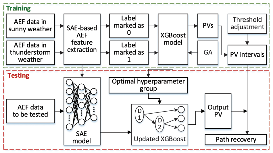
Figure 6: A flowchart of the proposed AEF testing method

3.3 Recovery Rule

The rules for thunderstorm path recovery are described as follows.

1)   Input of training model: Considering that SAE-XGBoost model requires a large amount of training data, the vertical AEF data from 00:00 to 20:00 every day of 7 sunny and 7 thunderstorm weathers in 2018 are selected as the training set (i.e., 72000 samples per day, totaling 1008000 samples), as is shown in Fig. 7.

2)   PV intervals corresponding to weather conditions: The strong data feature extraction abilities of SAE are adopted to extract the deep-seated AEF features. In addition, XGBoost is used to evaluate and classify the extracted features to obtain PV features. The distribution of PVs is presented in Fig. 8.

To visualize SAE-XGBoost model’s training results, all PV values are mapped as points in a 2D graph (Fig. 8). Among them, the red and blue points are obtained from the original AEF data in sunny and thunderstorm weathers, respectively. The horizontal and vertical coordinates of all these points are the values of 1-PV and PV respectively.

As shown in Fig. 8, on the basis of the threshold value 0.45 shown in the original green line, the threshold values of sunny and thunderstorm weathers are adjusted to the positions of red line and blue line respectively. Through this adjustment, negative effects of abnormal PVs on SAE-XGBoost model are effectively reduced. On this account, PV intervals SWI, II and TWI of sunny weather, between sunny and thunderstorm weather and of thunderstorm weather are (0, 0.2606), [0.2606, 0.6771] and (0.6771, 1) respectively. Note that this model is fixed for the subsequent path recovery.

3)   Path recovery implementation: The recovered AEF is input to the fixed SAE-XGBoost model, resulting in a PV output. If this PV belongs to TWI, the thunderstorm path fitting is further performed. Otherwise, no fitting is required.

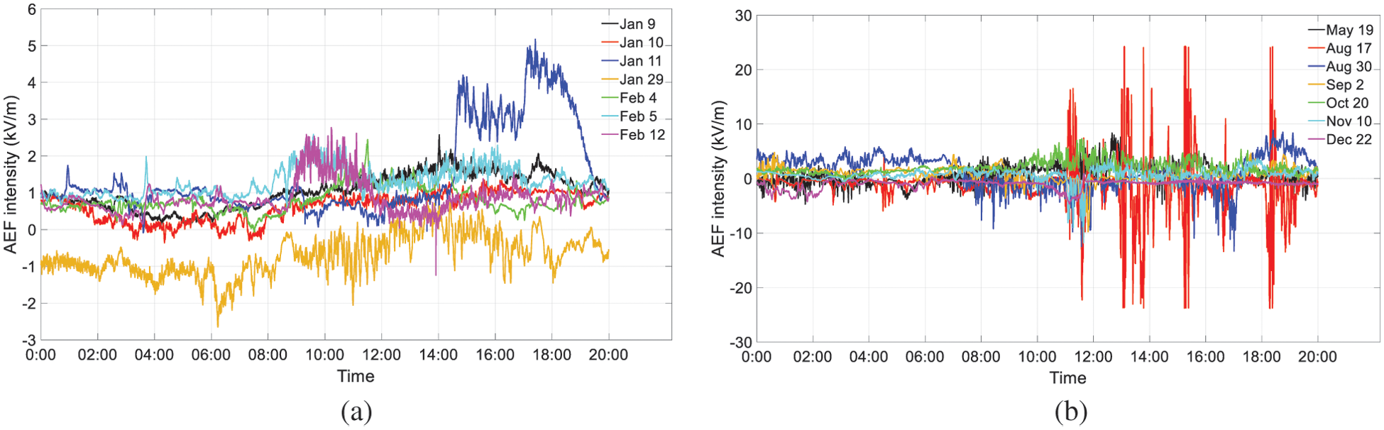
Figure 7: AEF data for training. (a) Data in sunny weather; (b) Data in thunderstorm weather

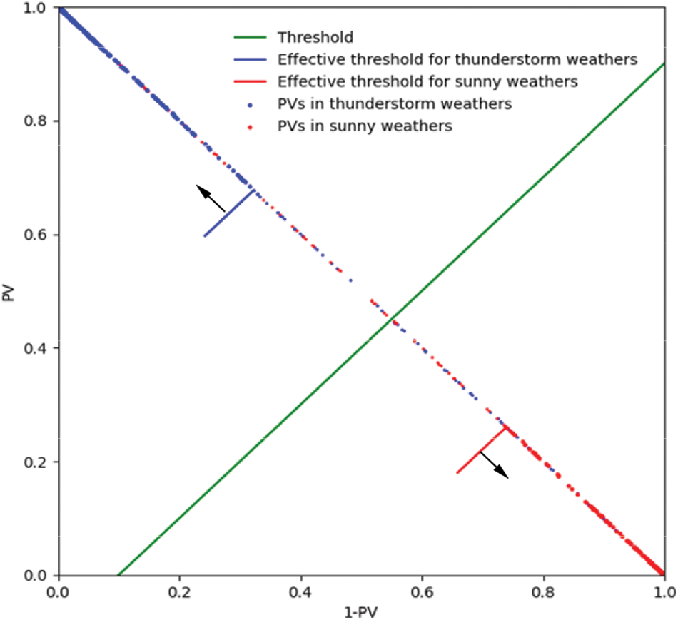
Figure 8: The distribution of PVs

4  Performance Evaluation

This section quantitatively evaluates the prediction and real-time performances to verify the effectiveness and complexity of the proposed method.

4.1 Prediction Effect Evaluation

Ez data of the first 100 min per day for the first three days in Fig. 4b are selected as samples numbered 1 to 3 respectively. Mean absolute error (MAE), mean absolute percentage error (MAPE), root mean square error (RMSE) and determining coefficient R2(%) are used as indexes to evaluate the prediction effects based on LSTM series methods (Table 1). The settings of learning rate, epochs, training and test set division, and optimizer are consistent with those of the proposed CNN-BiLSTM model.

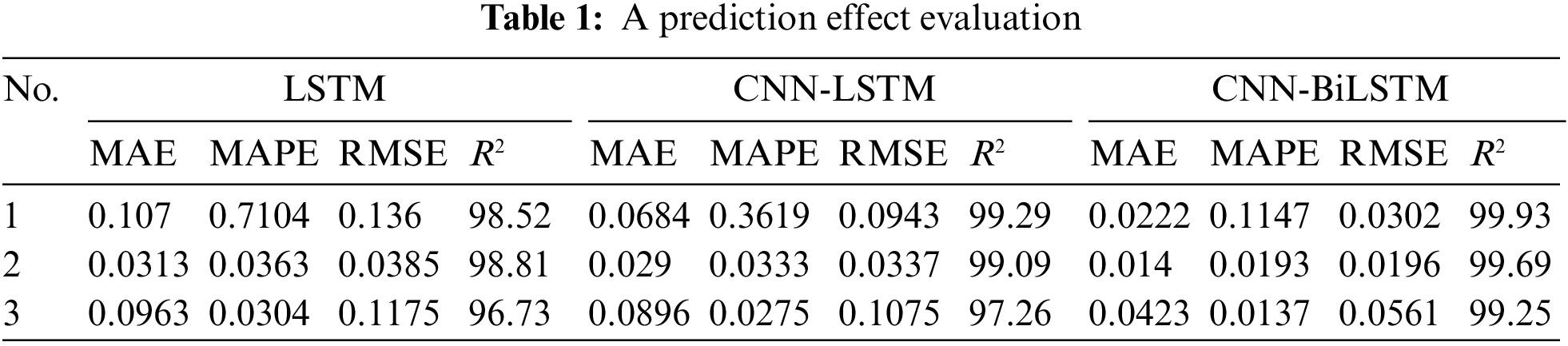
On the first sight, CNN-BiLSTM is the most competitive, and its MAE, MAPE, RMSE are the smallest, and R2 is the largest. CNN-LSTM is sub-optimal, while LSTM performs worst. Since CNN enhances the mining and extraction capabilities of effective data features, the maximum ratios of MAE, MAPE, RMSE reduction and R2 increase of CNN-LSTM compared to LSTM are 36.07%, 49.06%, 30.66%, and 0.78%, respectively. A further combination of BiLSTM makes the maximum ratio of CNN-BiLSTM’s MAE, MAPE, RMSE reduction and R2 increase compared to CNN-LSTM to 67.54%, 68.3%, 67.97%, and 2.05%, respectively. The proposed CNN-BiLSTM exhibits a more skillful prediction performance.

4.2 Real-Time Performance Evaluation

Based on samples in Table 1, the proposed method is tested on the processing time and graphics processing unit’s (GPU’s) occupancy rate (OR) (each sample is tested for 3 rounds). The relevant results are recorded in Table 2. Note that all processing is performed on a GPU mounted on an NVIDIA GeForce RTX3070 graphics card.

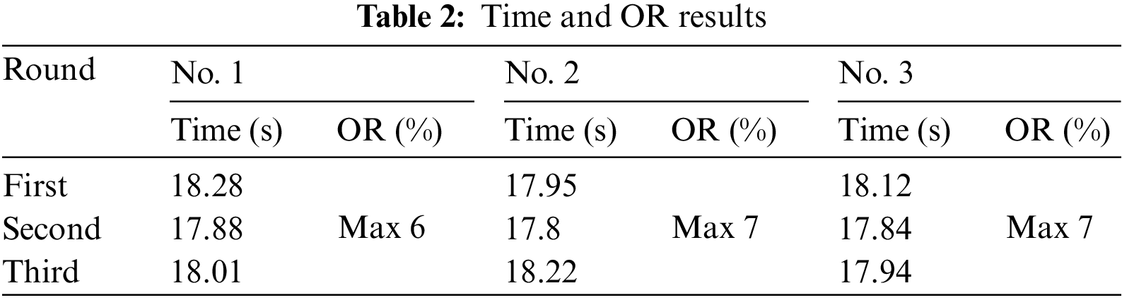
As is seen from Table 2, the processing time is between 17 and 19 s, and the maximum OR reaches 7%. For different samples, the proposed path recovery method displays a stable relative real-time performance, low complexity and high computation efficiency. In the thunderstorm detection system presented in [22], a 1-min interval AEF data read way is adopted. While our method meets the data processing efficiency required by this read way, the remaining large computing space is conducive to subsequent method expansion and parallel computing.

5  Results and Analyses

Comprehensive experiments are conducted in this section to verify the path recovery effectiveness applying the proposed method. Experiment implementation steps are described in Section 5.1. Two experiments are carried out in Sections 5.2 and 5.3, respectively. Contrast experiments are implemented in Section 5.4.

In Fig. 9, 3DAEFA is installed on the roof of School of Electronics and Information Engineering, Nanjing University of Information Science and Technology (NUIST). AEF data in this paper are all measured by this station.

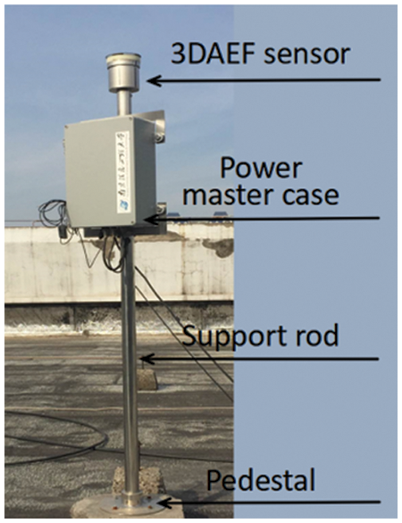
Figure 9: 3DAEFA in NUIST station

5.1 Experiment Implementation

The first step for the experiment implementation is to deploy 3DAEFA where the ground RP is low and there are no obvious protruding objects such as buildings, trees, communications base stations. The calibrated 3DAEFA has taken waterproof and anti-electricity measures beforehand. The second step is to check slave computer’s power supply, communication, etc. and upper computer’s (UC’s) response, setting, etc., and carry out a trial run. In the third step, the collected 3DAEF data are processed by UC, enabling reliable and efficient path recovery.

5.2 First Experiment

3DAEF data are adopted, from 00:00 to 01:40 on August 4, 2019, as shown in Fig. 10.

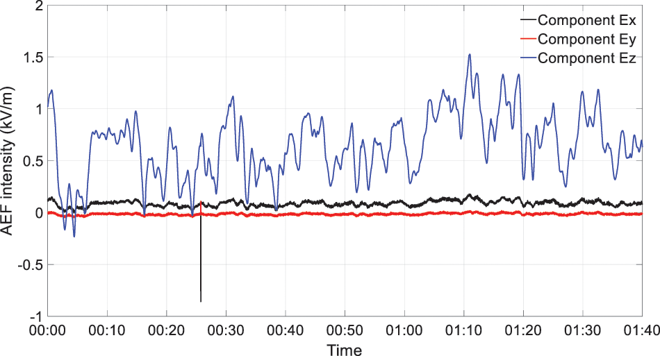
Figure 10: 3DAEF data from 00:00 to 01:40 on August 4, 2019

In Fig. 10, the amplitudes of components Ex, Ey and Ez are all small, with a maximum of about 1.5 kV/m. Among them, Ez fluctuates slightly. The amplitudes of horizontal components Ex and Ey are close to 0 and hardly change with time. Assuming that Ez from 01:10 to 01:40 is lost, AEF data recovered by CNN-BiLSTM are shown in Fig. 11.

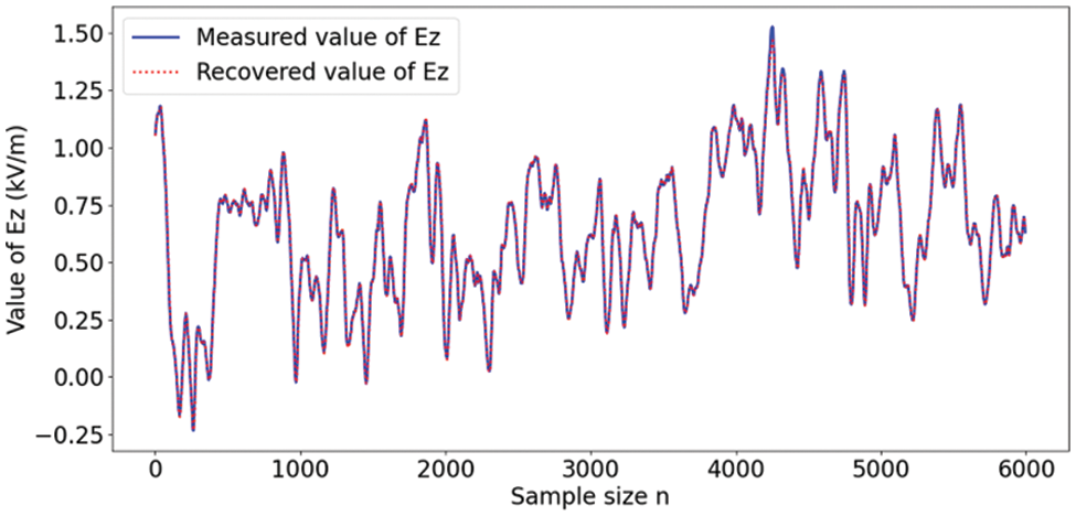
Figure 11: AEF recovery results in sunny weather

In Fig. 11, the recovered AEF shown by samples 4200 to 6000 (corresponding to 01:10 to 01:40) almost overlaps original AEF. The determination coefficient of 99.56% reflects that this AEF recovery has a good fitting degree. PV obtained using these results is 0.0405, which belongs to interval SWI. Therefore, no path fitting is required.

5.3 Second Experiment

3DAEF data are adopted, from 16:20 to 18:00 on August 4, 2019, as shown in Fig. 12.

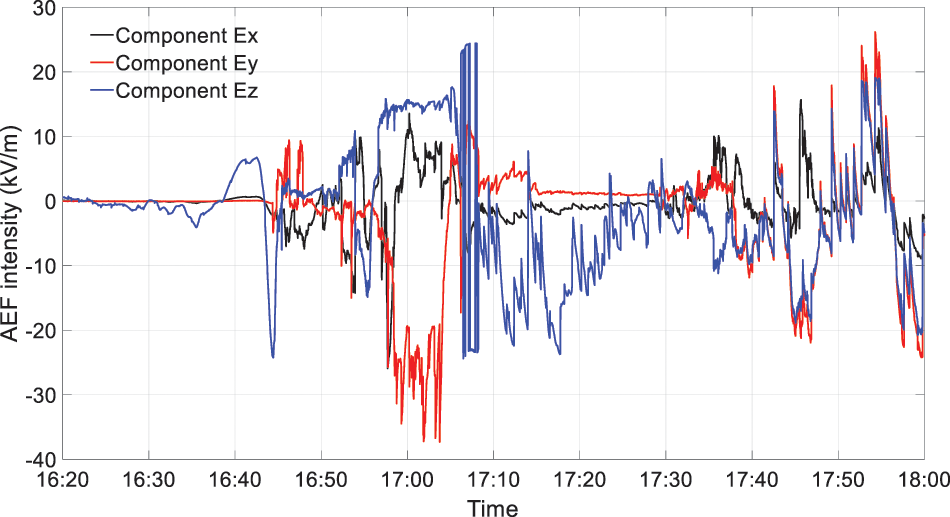
Figure 12: 3DAEF data from 16:20 to 18:00 on August 4, 2019

In Fig. 12, the fluctuations of components Ex, Ey and Ez are large, and the maximum amplitude is close to 40 kV/m. Even Ex, which displays a relatively small fluctuation, has a maximum amplitude of about 25 kV/m. Obviously, AEF during this period has weather attributes of thunderstorms. After assuming Ez loss from 17:30 to 18:00, the results of the recovered AEF are shown in Fig. 13.

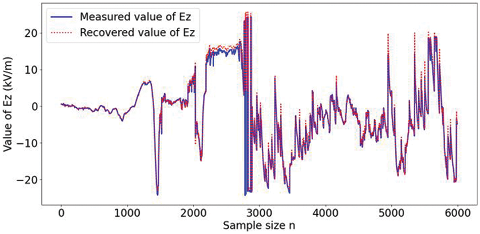
Figure 13: AEF recovery results in thunderstorm weather

In Fig. 13, the samples from 4200 to 6000 (corresponding to 17:30 to 18:00) show that the change trend of the recovered AEF is almost the same as original AEF. Although AEF fluctuation is relatively severe, 97% determination coefficient recorded still demonstrates better recovery effects [5]. Here, the output PV is 0.8114, which belongs to interval TWI. According to the rules in Section 3.3, thunderstorm point charge localization results are first recovered (Fig. 14). The color ranging from red to green indicates the thunderstorm processing from the beginning to the end.

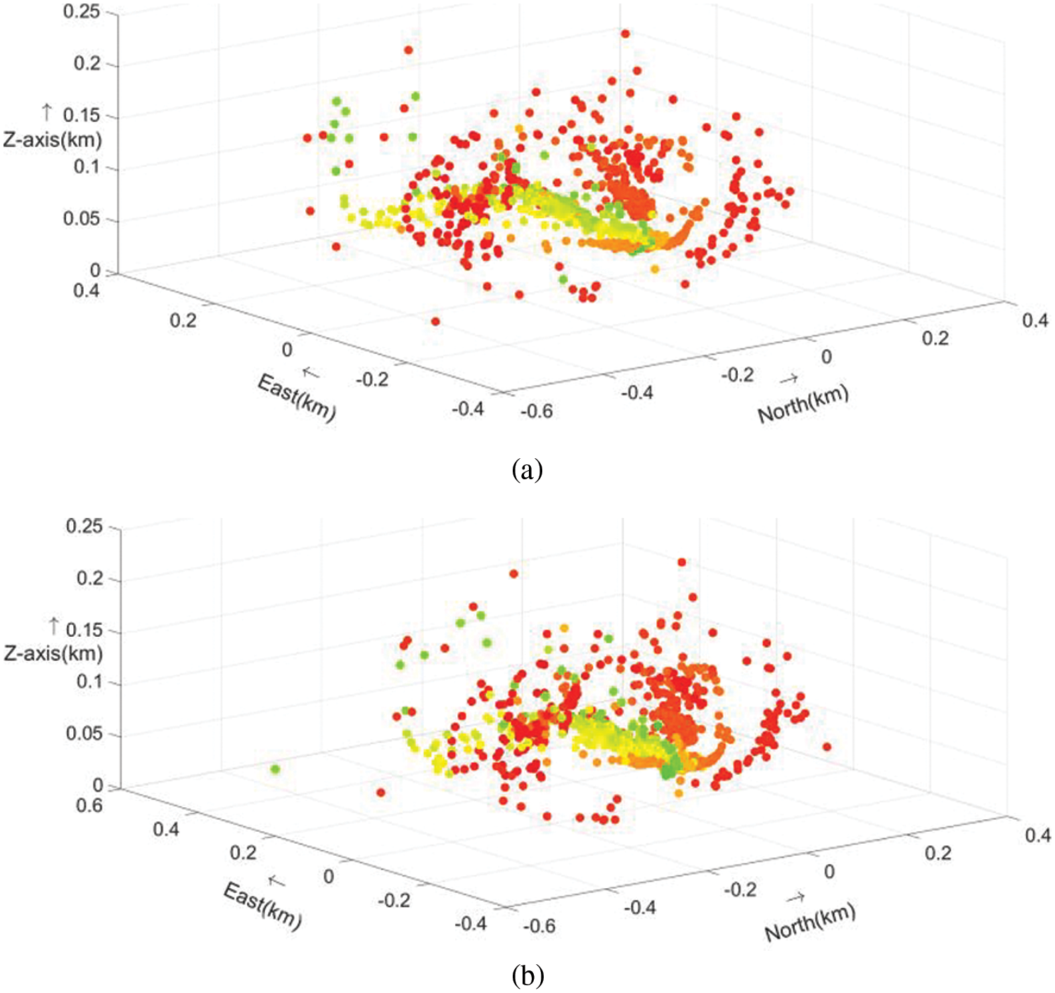
Figure 14: The thunderstorm point charge localization results. (a) Original localization results; (b) Recovered localization results

The recovered localization results in Fig. 14 are not significantly different from original localization results, according to charge aggregations with the same color. However, from this macro perspective, it is difficult to judge thunderstorm movements and developments, being it based on original or recovered results. Fig. 15 presents thunderstorm point charge moving paths.

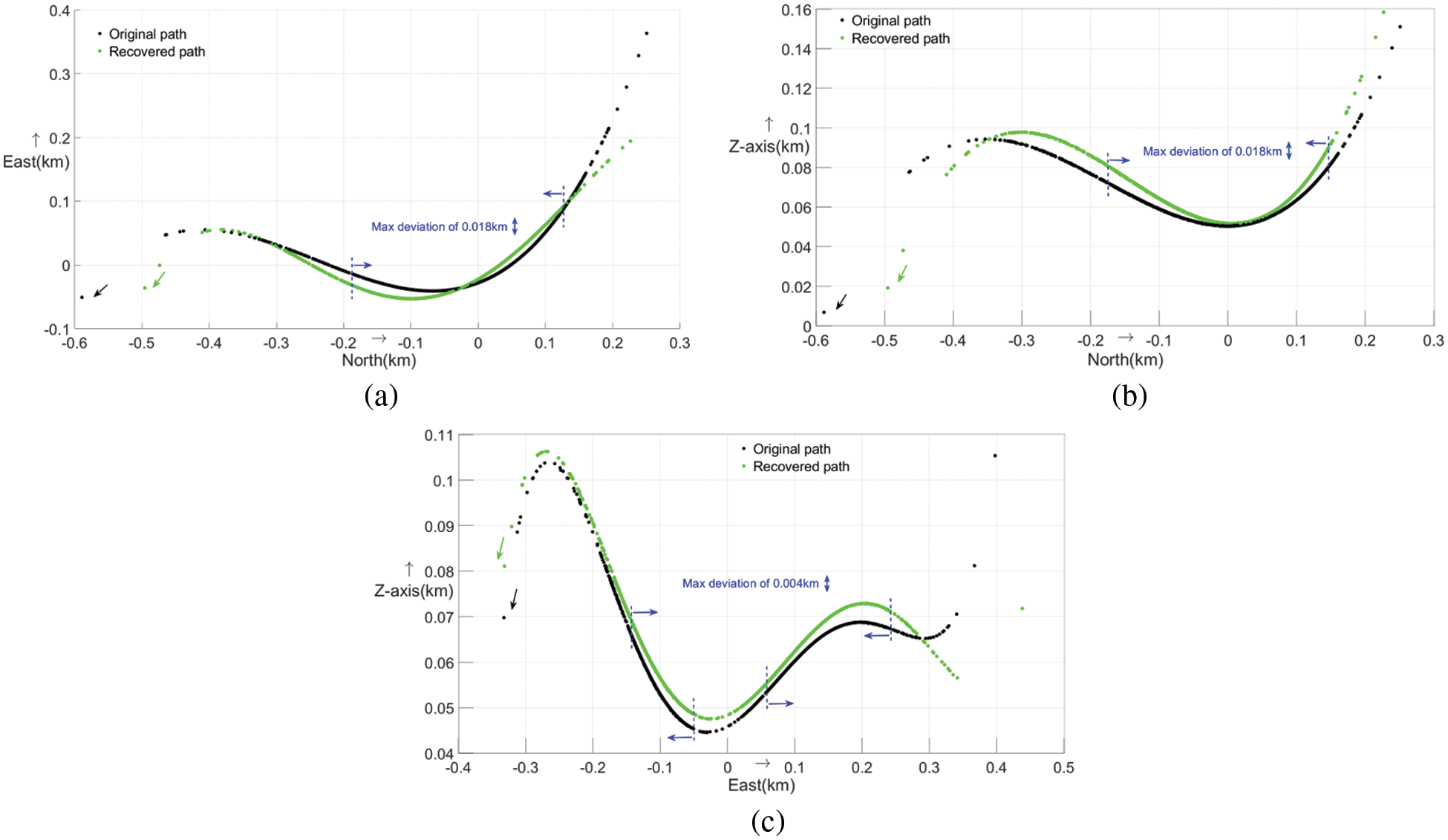
Figure 15: The thunderstorm path recovery results. (a) The top view of paths; (b) Paths in the north-south direction; (c) Paths in the east-west direction

In Fig. 15, the change trend of the original path (black line) and the recovered path (green line) remains roughly the same. The parts between blue dotted lines are used to study the maximum path deviation due to the path continuity and the dense distribution of path charges. Compared with the original path, the maximum deviation is about 0.018 km in the east-west direction of the recovered path shown in Fig. 15a. The maximum deviations are about 0.018 km and 0.004 km respectively in the Z-axis direction of paths in Figs. 15b and 15c. Generally speaking, deviations of no more than 0.018 km are at a low level, reflecting the proposed method’s effectiveness. In addition, as is seen from Fig. 15a, the thunderstorms gradually move to the southwest with time. Figs. 15b and 15c reveal the southward and westward thunderstorm motions respectively, which is consistent with the conclusion of Fig. 15a.

5.4 Contrast Experiments

As shown in Fig. 16, the radar charts matching AEF loss time in the second experiment are selected for comparative analyses. The blue cross marked in Fig. 16 is the NUIST Station position.

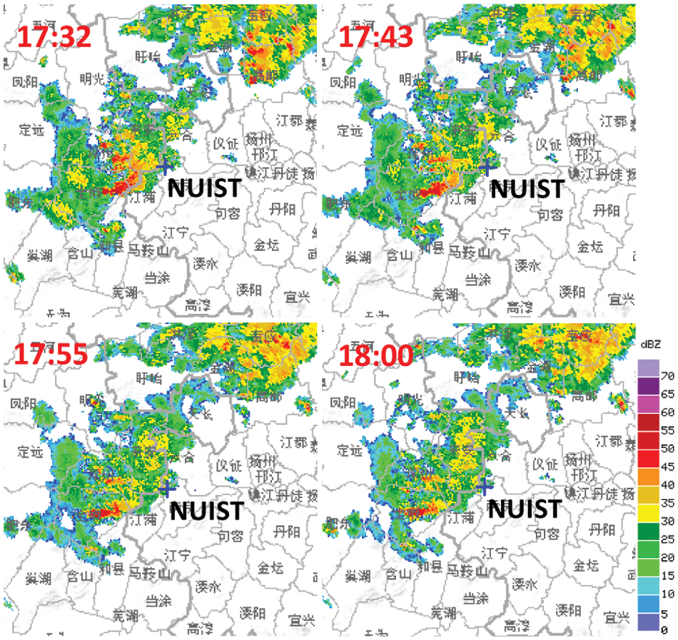
Figure 16: The radar charts of Nanjing radar station from 17:32 to 18:00 on August 4, 2019

In Fig. 16, there are two strong thunderstorm areas close to the station’s west and southwest areas, and corresponding radar echo intensities are not lower than 40 dBZ. From 17:32 to 18:00, the intensities above the station are not less than 30 dBZ. This indicates that thunderstorms are occurring around the station. Additionally, the thunderstorm core areas are moving away from the station and further southwest over time. This reduces thunderstorm intensities around the station, which in turn leads to a reduction in point charge height Z in later stages (as does the tail path height) [14,22]. This conclusion is well corroborated by Figs. 15b and 15c. The fact that thunderstorms move to the southwest as reflected in radar charts is consistent with analyses in Fig. 15.

The performances of this method and of those previously reported ones are summarized in Table 3.

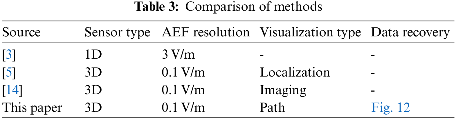
In Table 3, in terms of AEF resolution, [3] achieves 3 V/m, which is at a low level. References [5,14] and this paper all adopt a 3D single-axis rotary vane AEF sensor, and achieve a high AEF resolution of 0.1 V/m. Reference [3] uses a 1D field-grinding electric field meter, so 3DAEF fails to be acquired. This limits further visualization of thunderstorms. However, a point charge localization method proposed in [5] develops time-series AEF signals into a thunderstorm visual detection in space domains. On this account, [14] and this paper use localization results to perform curve fittings. This method is more conducive to the intuitive analyses of thunderstorm activities. Although references [3,5] and [14] do not carry out data recovery, [5] conducts AEF prediction. This provides an insight for the thunderstorm path recovery. In this paper, a CNN-BiLSTM model is established to predict and recover lost AEF data. In particular, the implementing path recovery necessity is judged with PV intervals, based on the designed SAE-XGBoost model. In short, the method proposed in this paper illustrates better performances in AEF data measurement and recovery, and thunderstorm visualizations.

6  Conclusion

A thunderstorm path recovery method is proposed, to reduce the negative effects of AEF data loss on thunderstorm detection. This method establishes a thunderstorm point charge localization model, deduces localization formulae, recovers AEF data, and realizes an effective point charge path recovery based on PV intervals. In particular, PV intervals are acquired by an established SAE-XGBoost model. This provides a criterion for judging the recovery implementation necessity. Both the feasibility of the proposed method and its effectiveness are soundly proved, against actual and contrast experiments. As to future advancements of the study, the fuzzy theories may be focused on further enhancing interpretability of results.

Funding Statement: This research is supported by a grant from State Key Laboratory of Resources and Environmental Information System, the National Natural Science Foundation of China, Grant Number 42201053, the Program of China Scholarship Council, Grant Number 202209040027, and the Postgraduate Research & Practice Innovation Program of Jiangsu Province, Grant Number KYCX21_1000, which are highly appreciated by the authors.

Conflicts of Interest: The authors declare that they have no conflicts of interest to report regarding the present study.

References

1. J. Yan, “Climatic characteristics of thunderstorm and its effect on agriculture,” Journal of Agricultural Catastrophology, vol. 8, no. 5, pp. 117–118, 2018. [Google Scholar]

2. X. Cheng, H. Zhu, K. Zhou and K. Wang, “Analysis of lightning characteristics during a disaster-causing thunderstorm in Anhui Province,” Torrential Rain and Disasters, vol. 37, no. 3, pp. 265–273, 2018. [Google Scholar]

3. A. Fort, M. Mugnaini, V. Vignoli, S. Rocchi, F. Perini et al., “Design, modeling, and test of a system for atmospheric electric field measurement,” IEEE Transactions on Instrumentation and Measurement, vol. 60, no. 8, pp. 2778–2785, 2011. [Google Scholar]

4. X. Yang, H. Xing, W. Xu and X. Ji, “A moving path tracking method of the thunderstorm cloud based on the three-dimensional atmospheric electric field apparatus,” Journal of Sensors, vol. 2021, pp. 1–13, 2021. [Google Scholar]

5. X. Yang, H. Xing and L. Zhuang, “A thunderstorm cloud point charge localization method based on CEEMDAN and SG filtering,” IEEE Access, vol. 9, pp. 17049–17059, 2021. [Google Scholar]

6. F. Esposito, R. Molinaro, C. Popa, C. Molfese, F. Cozzolino et al., “The role of the atmospheric electric field in the dust lifting process,” Geophysical Research Letters, vol. 43, no. 10, pp. 5501–5508, 2016. [Google Scholar]

7. H. Xing, G. He and X. Ji, “Analysis on electric field based on three dimensional atmospheric electric field apparatus,” Journal of Electrical Engineering and Technology, vol. 13, pp. 1696–1703, 2018. [Google Scholar]

8. Y. Zhang, H. Li, Z. Wang, W. Zhang and J. Li, “A preliminary study on time series forecast of fair-weather atmospheric electric field with WT-LSSVM method,” Journal of Electrostatics, vol. 75, pp. 85–89, 2015. [Google Scholar]

9. A. Karagioras and K. Kourtidis, “A study of the effects of rain, snow and hail on the atmospheric electric field near ground,” Atmosphere, vol. 12, no. 8, pp. 996, 2021. [Google Scholar]

10. A. Kamra and M. Ravichandran, “On the assumption of the Earth’s surface as a perfect conductor in atmospheric electricity,” Journal of Geophysical Research, vol. 98, no. 12, pp. 22875–22885, 1993. [Google Scholar]

11. H. Xing, X. Yang and J. Zhang, “Thunderstorm cloud localization algorithm and performance analysis of a three-dimensional atmospheric electric field apparatus,” Journal of Electrical Engineering and Technology, vol. 14, no. 6, pp. 2487–2495, 2019. [Google Scholar]

12. X. Zhang, Q. Bai, S. Xia, F. Zheng and S. Chen, “Miniaturized 3-D electric field sensor,” Chinese Journal of Scientific Instrument, vol. 27, no. 11, pp. 1433–1436, 2006. [Google Scholar]

13. T. Tantisattayakul, K. Masugata, I. Kitamura and K. Kontani, “Development of the hybrid electric field meter for simultaneous measuring of vertical and horizontal electric fields of the thundercloud,” IEEE Transactions on Electromagnetic Compatibility, vol. 48, no. 2, pp. 435–438, 2006. [Google Scholar]

14. X. Yang, H. Xing, X. Su and X. Ji, “Entropy-based thunderstorm imaging system with real-time prediction and early warning,” IEEE Transactions on Instrumentation and Measurement, 2022. [Google Scholar]

15. S. Guastavino, M. Piana, M. Tizzi, F. Cassola, A. Iengo et al., “Prediction of severe thunderstorm events with ensemble deep learning and radar data,” arXiv, 2021. [Google Scholar]

16. W. Xu, Z. Xia and H. Xing, “A lightning warning method based on EEMD and XGBoost,” Chinese Journal of Scientific Instrument, vol. 41, pp. 235–243, 2020. [Google Scholar]

17. W. Suparta, W. Putro and T. Darmastono, “Prediction of thunderstorm occurrences in tropical areas using a numerical model,” Geographia Technica, vol. 16, no. 1, pp. 78–86, 2021. [Google Scholar]

18. Z. Ni and T. Wen, “A weather prediction model based on CNN and RNN deep neural network-an example is the 6 hour forecast of thunderstorm in Beijing,” Journal on Numerical Methods and Computer Applications, vol. 39, no. 4, pp. 299–309, 2018. [Google Scholar]

19. M. Lin, “Research on prediction model of lightning activity based on improved fuzzy neural network,” M.S. Dissertation, Xidian University, China, 2014. [Google Scholar]

20. Y. Cui and X. Hu, “Lightning activity prediction based on IFCM-T-S,” Foreign Electronic Measurement Technology, vol. 38, no. 7, pp. 12–16, 2019. [Google Scholar]

21. W. Xu, C. Zhang, X. Ji and H. Xing, “Inversion of a thunderstorm cloud charging model based on a 3D atmospheric electric field,” Applied Sciences, vol. 8, no. 12, pp. 2642, 2018. [Google Scholar]

22. X. Yang, H. Xing, W. Xu, X. Ji and X. Su, “3DAEFA-based thunderstorm prediction system with higher performance,” IEEE Sensors Journal, vol. 22, no. 23, pp. 22865–22884, 2022. [Google Scholar]

23. S. Xie, B. Shao and H. Sheng, “Field mill type atmospheric electric field apparatus and its calibration system,” Journal of Zhejiang Meteorology, vol. 34, no. 3, pp. 36–38, 2013. [Google Scholar]

24. C. Gan, Q. Feng and Z. Zhang, “Scalable multi-channel dilated CNN-BiLSTM model with attention mechanism for Chinese textual sentiment analysis,” Future Generation Computer Systems, vol. 118, pp. 297–309, 2021. [Google Scholar]

25. J. Yang, K. Sim, X. Gao, W. Lu, Q. Meng et al., “A blind stereoscopic image quality evaluator with segmented stacked autoencoders considering the whole visual perception route,” IEEE Transactions on Image Processing, vol. 28, no. 3, pp. 1314–1328, 2019. [Google Scholar]

26. Y. Sha, J. Faber, S. Gou, B. Liu, W. Li et al., “An acoustic signal cavitation detection framework based on XGBoost with adaptive selection feature engineering,” Measurement, vol. 192, pp. 110897, 2022. [Google Scholar]

27. D. Zhao, H. Xing, H. Wang, H. Zhang, X. Liang et al., “Sea-surface small target detection based on four features extracted by FAST algorithm,” Journal of Marine Science and Engineering, vol. 11, no. 2, pp. 339, 2023. [Google Scholar]