A Health State Prediction Model Based on Belief Rule Base and LSTM for Complex Systems

1  Introduction

The complexity of the industrial system has gradually increased with the advancement of science and technology, and the working environment has become harsher. Especially in the fields of aerospace and weaponry [1,2], the reliability and safety of the system are crucial. Once the health state changes and serious accidents occur, it will not only cause huge damage to the environment but also bring bad effects to society. In order to cut maintenance costs and prevent significant safety incidents, it is required to predict the health state of complex systems [3,4].

Health state prediction of complex systems refers to the prediction of the future health state by considering the historical and current health state of the system. There are three different kinds of approaches are used for health state prediction in recent research: analytical model-based [5], data-driven-based [6], and semi-quantitative information-based methods [7].

Once the analytical model of the system is known, the analytical model-based method like the particle filter can investigate the law of the health state degradation and predict changes in the health state in the future [8–10]. Once the system collects a significant amount of observed information, data-driven-based methods like LSTM and support vector machine (SVM) model can be established the relationship between quantitative data of the system and the health state at future moments to achieve the effect of prediction [11–13]. Once the qualitative knowledge of the system and some of the observed data are known, semi-quantitative information-based methods can be used to implement the prediction process, which includes the Hidden Markov modeling-Bayesian networks (HMM-BN) [14], fuzzy system-gray model-support vector machine (FS-GM-SVM) model [15], and so on.

In recent years, many scholars have conducted research on the health state prediction for the complex system. Liu et al. constructed an underdetermined extended Kalman filter and applied it to the health state estimation of aero engines to solve the problem of less available sensor data and more unknown parameters [16]. Zhang et al. designed a weight optimization unscented Kalman filter (WOUKF) to establish a trend of prediction residuals between the WOUKF and the true capacity, which is used to update the model parameters within the prediction cycle to improve the prediction performance [17]. Liao et al. proposed a flexible prediction framework based on the high-order hidden semi-Markov model (HSMM) that extends the basic HSMM for systems or components with unobservable health states and complex transition dynamics [18]. Pan et al. proposed a chaotic prediction model for vibration data based on improved SVM swarm optimization to improve the prediction accuracy of pump operation state, obtained the training set by phase space reconstruction, and optimized the parameters of the SVM using an improved particle algorithm [19]. Xu et al. established a prediction method for onboard integrated health management system state assessment of manned spacecraft aerospace equipment and used FS-GM-SVM model for prediction to address the uncertainty of the prediction process [15]. Soleimani et al. proposed a fault prediction method based on the integration of HMM and BN to address nonlinear and non-Gaussian data features [14].

However, all the above-predicted methods have a specific scope of application. The working mechanism of most complex systems is difficult to analyze, and it is hard to build a reliable analytical model. As a black-box model, the prediction process of data-driven-based methods is not transparent, which makes the results lack interpretability. The prediction accuracy of semi-quantitative information-based methods cannot be guaranteed if the observed information of the system is disturbed. In addition, most papers use a single indicator to predict the health state. Complex systems have multiple indicators with complex coupling relationships. It is difficult for a single indicator to accurately depict the health state, and it is necessary to fuse multiple indicators for prediction. In this paper, the belief rule base (BRB) is chosen to fuse expert knowledge, system mechanism, and multi-indicator data to improve the accuracy and interpretability of prediction. The BRB can effectively handle multi-source information to achieve the modeling of the complex system [20,21]. The reasoning process is clear and transparent, and the reasoning results are easy to interpret and analyze [22]. The engineering practice demonstrates that the BRB performs effectively in the health state prediction of aero engines [23]. Hu et al. designed a prediction model based on time-delay hidden BRB (THBRB), which considers the multi-moment instantaneous input of HBRB, can better express the influence of historical data, and improves the prediction capability of traditional HBRB [24]. Chen et al. established a transmission mechanism health state prediction method based on BRB for transmission mechanism system and used singular value decomposition to realize multi-sensor information fusion as the input of the prediction model, which effectively predicted the health condition of the transmission mechanism system [25].

Most of the above studies use BRB as a time series forecasting model together with an indicator fusion model, however, when there is a long-term dependence problem in the time series, i.e., the values of multiple historical moments need to be used to predict the next moment, BRB will create a “combinatorial explosion” problem, and it is difficult to determine the corresponding parameters based on the relationship between the values of multiple moments. Therefore, it is necessary to choose a more suitable time series forecasting model to predict the indicators. As an important parameter of the BRB, the reasonableness of setting the referential values of indicators determines the effectiveness of the model. The referential values of indicators are usually given by the expert. Since only the current system working condition is considered, the referential values given by the expert cannot fully reflect the future system working conditions, resulting in large errors between the model output and the actual system. How to reasonably determine the referential values of indicators is a problem to be considered.

Based on the above analysis, a health state prediction model based on BRB and LSTM for complex systems is constructed in this paper. LSTM performs better than BRB in long-term reliance issues and has great time series processing and prediction capabilities, and is widely used and solved in various fields such as machinery, energy, and medicine [26,27]. The predicted values of indicators are obtained using the LSTM and provided input information for the BRB. The Density Peak Clustering (DPC) algorithm is able to select representative points and uses them as referential values of indicators [28]. The referential values of indicators are determined by the DPC algorithm to establish the BRB and the health state prediction results are obtained using the BRB.

The remainder of this essay is structured as follows. In Section 2, a health state prediction model for complex systems and basic knowledge are introduced. In Section 3, the modeling procedure of the health state prediction model based on BRB and LSTM for complex systems is investigated. In Section 4, the effectiveness of the model is evaluated using the example of a certain vehicle hydraulic pump. The paper is concluded in Section 5.

2  Health State Prediction Model for Complex Systems and Basic Knowledge

In Subsection 2.1, the health state prediction model for complex systems is briefly introduced. In Subsection 2.2, the basic knowledge of the model is formulated.

2.1 Description of Health State Prediction Model

The health state of complex systems is affected by numerous factors, but some indicators can show changes in the health state. A health state prediction model is suggested in this paper. Based on historical and current observed data of indicators to calculate the predicted values. At the same time, the uncertainty of expert knowledge is considered to build the BRB, and the multi-source information is fused to achieve prediction, which makes the predicted process more comprehensive and reliable. Suppose the system has M indicators x1,x2,…,xM, the model framework is displayed in Fig. 1.

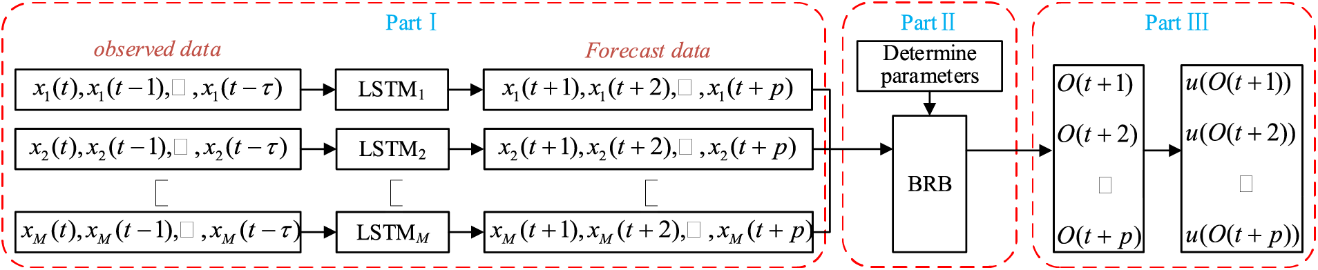
Figure 1: Framework of model

The model is composed of three sections. In part I, the predicted values of system indicators are obtained using LSTM. In part II, the BRB parameters are determined based on DPC algorithm and the BRB is built by expert knowledge. In part III, the results of the system-distributed prediction are obtained by inference, and the expected utility can be calculated. The following are explanations for each variable in Fig. 1.

1) τ represents the number of delay steps.

2) M indicates the number of indicators.

3) p represents the number of predicted steps.

4) O(⋅) represents the distributed health state prediction results.

5) u(O(⋅)) is the expected utility of O(⋅).

2.2 Basic Knowledge

2.2.1 Basic Knowledge of LSTM

LSTM has great time series processing and prediction capabilities and has a wide range of applications in finance, machinery, industry, etc. The networks can solve the problem of short-term memory in Recurrent Neural Networks (RNN), a large number of papers have introduced LSTM and solved various problems, and it is still widely used until now.

The key to LSTM is the cell state and the “gate” structure. The cell states act as the transmission chain of information, and only part of the linear interaction is involved, maintaining the integrity of the information. Theoretically, the information in the time series can be transmitted all the way through. The “gate” structure has four interaction layers, including three Sigmoid layers and one Tanh layer, which interact in a special way to control the increase and decrease of information. The “gate” structure contains forgetting gates, input gates, and output gates.

The retention and deletion of information are determined by the forgetting gate. The forgetting gate receives information about the concealed state of the preceding layer and information about the present situation, a nonlinear mapping relationship is established by the Sigmoid function σ, and the output vector ft is obtained. ft Between 0 and 1, 0 means all deletion and 1 means all retention. The forgetting gate can be expressed as:

ft=σ(Wf×[ht−1,xt]+bf)(1)

where Wf is the weighting matrix. ht−1 is the information of the hidden state of the previous layer. xt is the information at the current moment. bf is the bias.

The update of the cell state is determined by the input gate. The Tanh function is used to build a new vector of marquee values C~t when the Sigmoid function produces the output vector it and the information about the hidden state of the previous layer and the current moment is input. The old state Ct−1 of the cell is multiplied with ft to remove the unwanted information. C~t is multiplied with it to retain the desired information and finally summed to obtain the updated cell state Ct. The input gate can be expressed as:

it=σ(Wi×[ht−1,xt]+bi)(2)

C~t=tanh⁡(WC×[ht−1,xt]+bC)(3)

Ct=ft×Ct−1+it×C~t(4)

The hidden state contains the information from the previous time series and is determined by the output gate. The output vector ot is obtained by the Sigmoid function, which determines the information to be output. The cell state Ct is processed using the Tanh function and multiplied with the output vector ot to obtain the new hidden state information ht for output to the next layer. The output gate can be expressed as:

ot=σ(Wo×[ht−1,xt]+bo)(5)

ht=ot⊙tanh⁡(Ct)(6)

where ⊙ is the convolution.

2.2.2 Basic Knowledge of BRB

When assessing the future health state of the system, the k th rule can be described as follows:

Rk:If(x1 is A1k)∧⋯∧(xM is AMk)then {(D1,β1,k),…,(DN,βN,k)}with rule weight θkand indicator weight δ1,δ2,…,δM(7)

where xi(i=1,2,…,M) is the i th indicator, M is the number of indicators. Aik(k=1,2,…,L) is the i th referential value of the k th rule, L is the number of rules. Dn(n=1,2,…,N) is the n th consequent, N is the number of consequents. βn,k is the belief degree that the k th rule assigned to the n th consequent. θk is the weight of the k th rule, it shows how significant the k th rule is in comparison to other rules. δi is the weight of the i th indicator, it shows how significant the i th indicator is in comparison to other indicators.

3  Establishment of Health State Prediction Model Based on BRB and LSTM for Complex Systems

In Subsection 3.1, the LSTM-based predicted model of indicators is constructed. In Subsection 3.2, the DPC-based referential values of indicators determination and distance-based input information conversion method are proposed. In Subsection 3.3, the process of BRB build and reasoning are described. In Subsection 3.4, the modeling procedure of the health state prediction model based on BRB and LSTM for complex systems is summarized.

3.1 Construction of LSTM-Based Predicted Model of Indicators

The LSTM is used to predict the observed data of the indicators, the detailed steps are as follows:

1) Pre-processing of data

Prior to prediction, training data must be standardized, it can be calculated by:

xN(t)=x(t)−μ~σ~(8)

The alternating time step is utilized to process the training data, and the observed data from the previous time is used as an input to predict the observed data from the following time. Select to alternate a time step, which is written as:

{X1N={xN(1),xN(2)…,xN(t−1)}X2N={xN(2),xN(3)…,xN(t)}(9)

2) Definition and training of networks

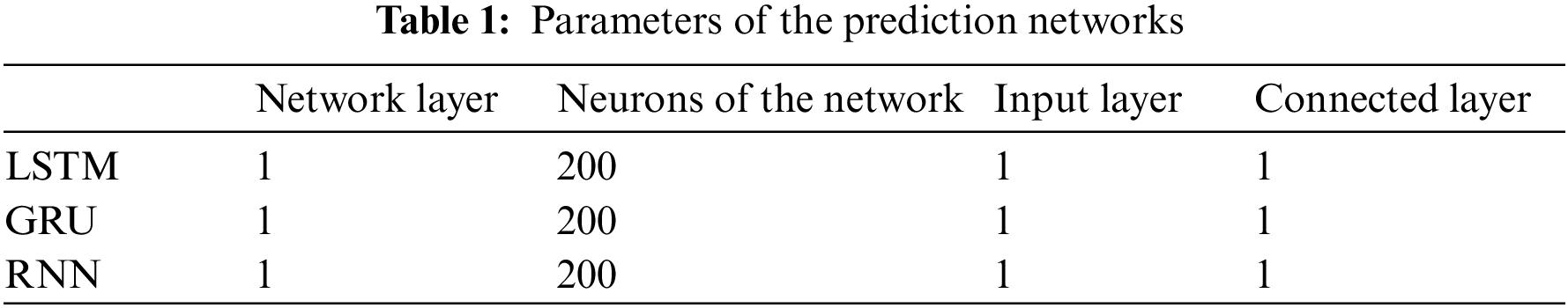
The dimensionality of the input determines the input layer, the dimensionality of the output determines the fully connected layer, and the data determines the number of neurons of the network.

After the structure has been defined, an appropriate optimizer must be selected to improve the learning effect. The Adaptive Moment Estimation (Adam) optimizer is used in this paper to adjust the learning rate during training and improve the convergence rate.

3) Prediction of indicators

The final step xN(t) is utilized to predict the first predicted value. To finish the prediction of indicators, the number of prediction steps need to be determined and the first predicted value is entered into the network.

3.2 Method of DPC-Based Referential Values Determination and Distance-Based Input Information Conversion

3.2.1 Determination of Referential Values

Referential values of indicators are an important parameter in the BRB. If the referential value is set unreasonably, the model accuracy will be greatly reduced. If there are too many referential values set, the rules will expand exponentially, thus making the calculation more difficult.

Suppose a system has two indicators A and B, each with three referential values A1,A2,A3 and B1,B2,B3. The rules are combinations of referential values, so the BRB of the system consists of 9 (3 × 3) rules, as depicted in Fig. 2.

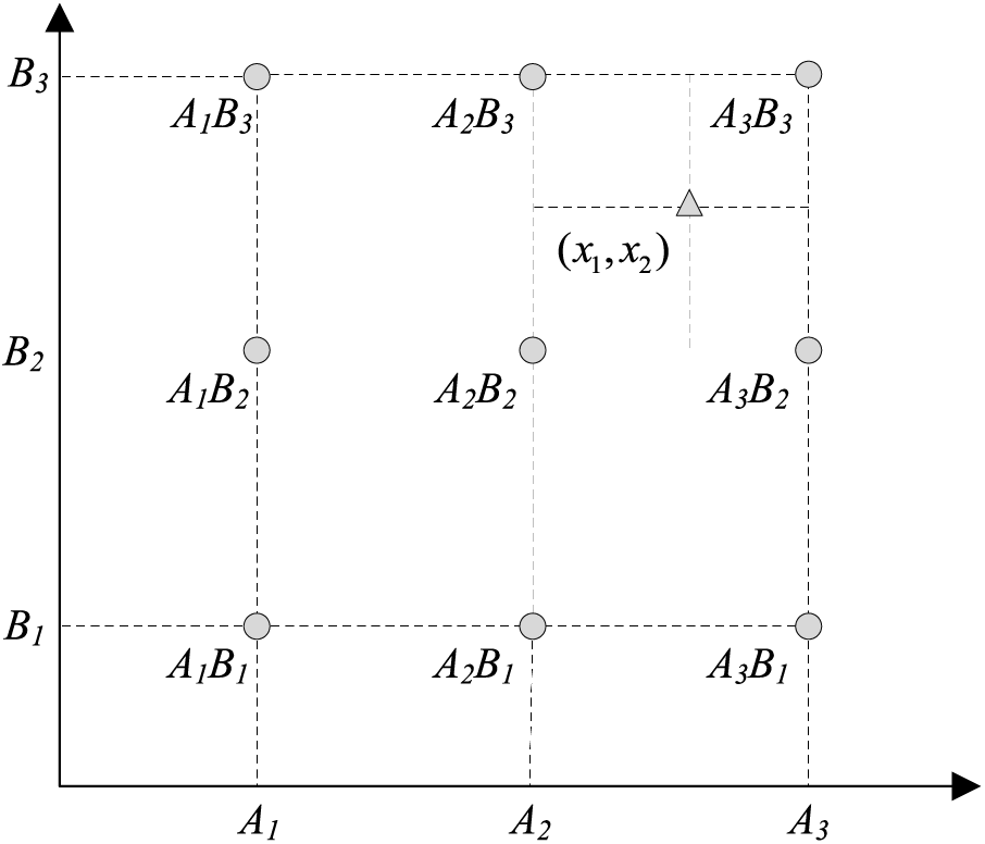
Figure 2: Relationship between input and activation rule

Where (x1,x2) is an input that activates the adjacent 4 rules A2B2, A2B3, A3B2 and A3B3.

Suppose that the health state corresponding to the values of x1 and x2 is medium. The referential values are not set properly, resulting in x1and x2 to activate rules corresponding to other health states. The matching degree of the medium health state is reduced, which affects the prediction accuracy of the model.

Therefore, the referential values should be chosen as a representative point surrounded by a sufficient number of points. The DPC-based method for determining referential values of indicators in this paper. The DPC algorithm is predicated on the idea that, for a given data set, the cluster center is enclosed by a few low-density data points which are far away from high-density data points. For the set S={X1;X2;…;Xm,Xm={x1(m),x2(m),…,xM(m)}} composed of each predicted value, the following are the steps of clustering.

1) Calculation of local density

The local density is calculated using a Gaussian kernel.

ρi=∑j=1me−(dijdc)2,i≠j(10)

where dij is the Euclidean distance between Xi and Xj. dc is a pre-specified distance threshold (The threshold is often set at the first 1% to 2% of the distance between all data points).

2) Calculation of minimum distance

εi=minρi<ρj{dij}(11)

where εi is the shortest distance between Xi to a higher local density data point Xj.

The maximum distance between Xk and the other data points is defined as εk for Xk with the highest global density.

3) Determination of clustering center

In the DPC algorithm, data point with both large ρi and εi is a potential clustering center. Combining the values of ρi and εi to νi, which is defined as follows:

νi=ρ¯iε¯i(12)

ρ¯i=ρimax(ρi)(13)

ε¯i=εimax(εi)(14)

νi of each data point is arranged in descending order, and the probability of being the cluster center increases with increasing νi.

The mean value ν¯ of νi is obtained, and the data point which νi exceeds ν¯ is selected as the potential clustering center. The slope trend of νi is used tri to determine the cluster center, defined as follows:

tri=(νi−1−νi)(νi−νi+1),i>1(15)

From the last clustering center to the first non-clustering center, there is a sharp decreasing tendency. The largest point tri is selected, and the first i−1 points are the cluster centers, noted asY={Y1;Y2;…;Yi−1,Yi−1={yi−11,yi−12,…,yi−1M}}. The components of each cluster center are arranged in ascending order and distributed to referential values of indicators in the BRB.

{A1={y11,y21,…,yi−11}A2={y12,y22,…,yi−12}⋮AM={y1M,y2M,…,yi−1M}(16)

3.2.2 Conversion of Input Information

In this paper, the input information is quantitative. The method of distance-based input information conversion is used, which is calculated as follows:

1) If xi is less than the minimum of referential value Ai1, the matching is 1 relative to Ai1 and 0 relative to the others. It can be denoted by:

{αi1=1αij=0,j≠1,xi<Ai1(17)

where αij represents the matching degree of xi relative to Aij.

2) If xi is more than the maximum of referential value AiJ, the matching is 1 relative to AiJ and 0 relative to the others. It can be denoted by:

{αiJ=1αij=0,j≠J,xi>AiJ(18)

3) If xi∈[Aij,Aij+1], it can be calculated by:

{αij=Aij+1−xiAij+1−Aijαij+1=1−αijαis=0,s≠j,j+1,Aij≤xi≤Aij+1(19)

3.3 Establishment and Inference of BRB

The expert set weights for each indicator, and combine the referential values of indicators to build BRB and set weights and belief degrees of results for each rule. Once the BRB has been established, inference can be made on the predicted values. The inference process is as follows:

1) Calculation of matching degree

When input xi is available, the matching degree of xi relative to the referential value is calculated according to (17)–(19).

2) Calculation of rule activation weight

The matching degree of xi needs to be fused with indicator weight and rule weight. The activation weight ωk is described as follows:

ωk=θk∏i=1M(αik)δ¯i∑l=1Lθl∏i=1M(αik)δ¯i(20)

δ¯i=δimaxi=1,2,…,M{δi}(21)

3) Integration of rules

The Evidential Reasoning (ER) approach is used to merge multiple activated rules, it can be denoted by:

βn=μ×[∏k=1L(ωkβn,k+1−ωk∑i=1Nβi,k)−∏k=1L(1−ωk∑i=1Nβi,k)]1−μ×[∏k=1L(1−ωk)](22)

μ=[∑n=1N∏k=1L(ωkβn,k+1−ωk∑i=1Nβi,k)−(N−1)∏k=1L(1−ωk∑i=1Nβi,k)]−1(23)

where βn is belief degree of the n th consequent, and 0≤βn≤1.

The distributed health state prediction results and expected utility are described as follows:

O(t+p)={(Dn,βn)}(24)

u(O(t+p))=∑n=1Nu(Dn)⌊βnmax{βn}⌋(25)

where ⌊⋅⌋ is rounded down.

3.4 Modeling Procedure of Health State Prediction Model Based on BRB and LSTM

The specific steps of the health state prediction model based on BRB and LSTM are shown in Fig. 3.

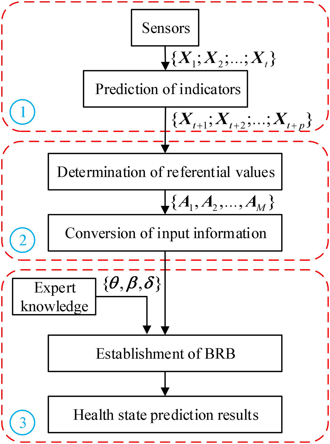
Figure 3: Modeling procedure of model

Step 1: Acquisition of observed data by sensors and calculation of predicted values of indicators by the method proposed in Subsection 3.1.

Step 2: Determination of referential values of indicators and conversion of input information.

Step 2.1: Determination of the cluster centers according to (10)–(15) and assignment of the cluster centers to referential values of indicators according to (16).

Step 2.2: Calculation of the matching degree according to (17)–(19).

Step 3: The expert provides parameters and builds BRB, and the health state prediction results are obtained using the BRB.

Step 3.1: Calculation of the rule activation weight according to (20) and (21).

Step 3.2: Calculation of the health state prediction results according to (22)–(25).

4  Case Study

In this section, the effectiveness of the model is demonstrated using an example from a certain vehicle hydraulic pump. The hydraulic pump draws oil from the hydraulic tank, forms pressure oil, and discharges the pressure oil to the actuating element. The hydraulic pump is usually composed of a pump body, hydraulic, cylinder, bearing, and other components. The principle of operation is that the movement brings about a change in the volume of the pump chamber, thus compressing the fluid so that the fluid has pressure energy.

The health state is highly unstable because of the complicated structure of the hydraulic pump and the varied working environment. The components of the hydraulic pump will age and wear while it operates, changing the health state. Therefore, to provide support for maintenance decisions for the hydraulic pump and prevent serious safety incidents, it is required to predict the health state.

Before making a prediction, a system of indicators related to the health state needs to be constructed. The indicators should accurately and thoroughly indicate the state of the system’s operation. The outlet pressure and outlet flow of the hydraulic pump are used as the input indicators, which combines expert knowledge and system mechanism.

Remark 1: Due to pressure, hydraulic oil leakage may occur from the gap between the combined surfaces of the hydraulic pump, and leakage may also be caused by worn piping or poorly connected hydraulic components. Oil leakage can lead to a reduction in outlet pressure and outlet flow, affecting stability and work efficiency, which can lead to failure.

4.1 Prediction of Indicators

A pressure sensor and a flow sensor were selected for the test, and a total of 260 sets of data were collected, as shown in Fig. 4.

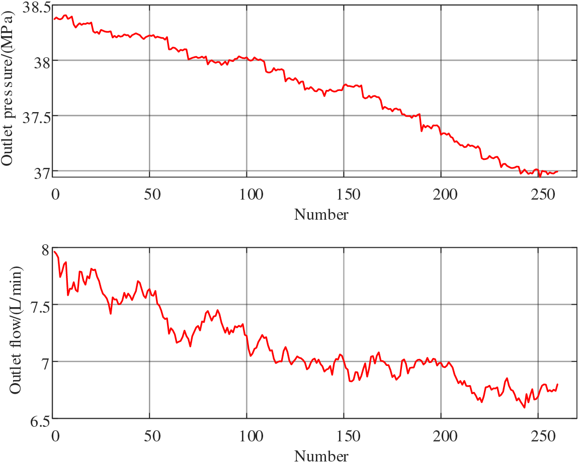
Figure 4: Observed data

The outlet pressure and outlet flow are predicted by LSTM, the number of predicted steps p=1. To verify the prediction effect, the LSTM is compared with the commonly used prediction networks Gate Recurrent Unit (GRU) and Recurrent Neural Network (RNN). The optimizer is selected as Adam, the network structure and training parameters are adjusted to optimize each method. The network settings are shown in Table 1.

By comparing the Mean Square Error (MSE) in Table 2 and the comparative results in Fig. 5, the error of LSTM is significantly smaller than GRU and RNN and has a higher prediction accuracy.

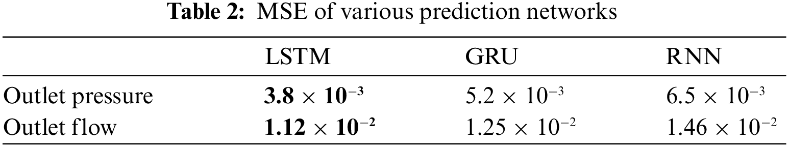
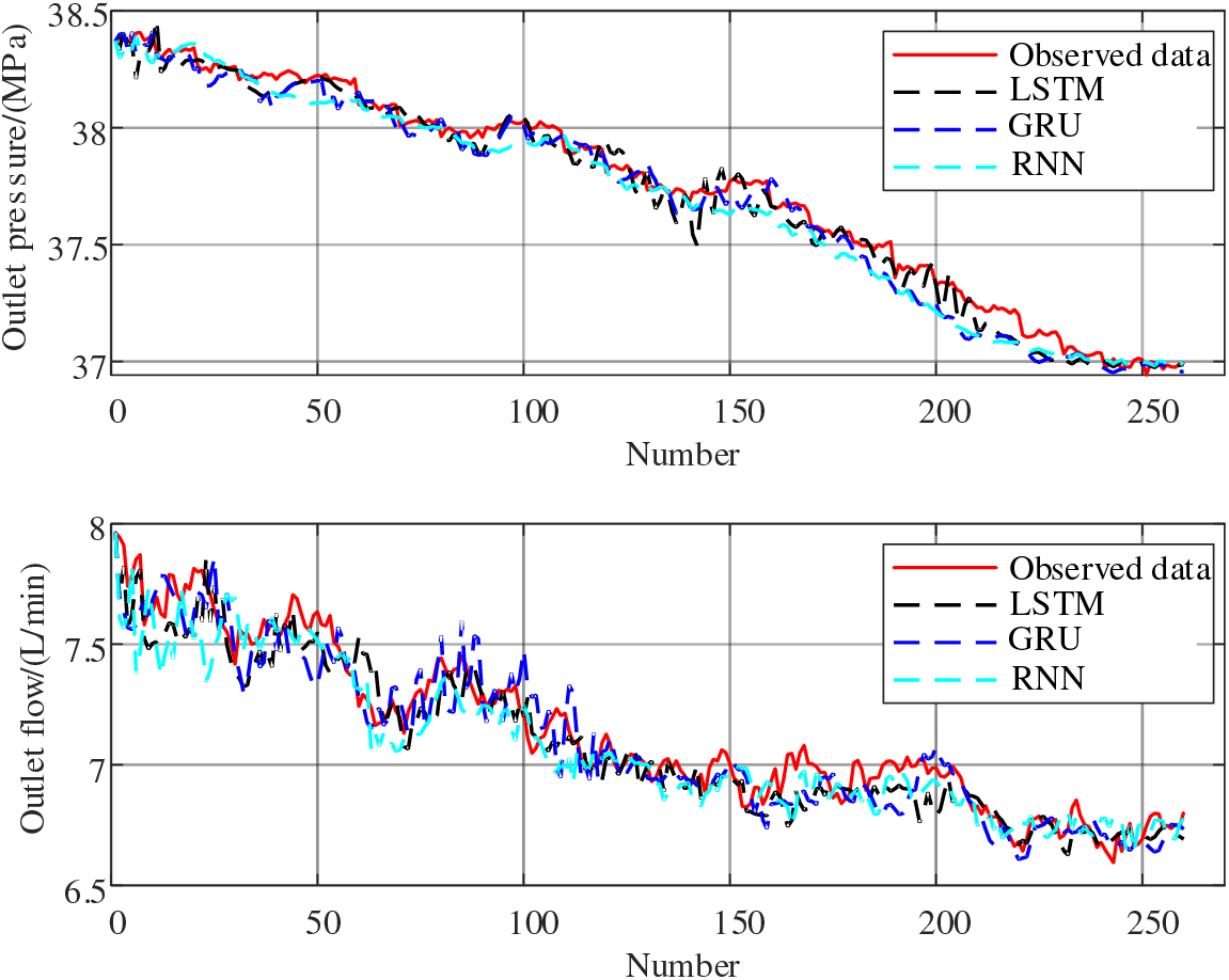
Figure 5: Comparison of various prediction networks

Remark 2: As can be seen from Fig. 5, compared with the real data, the prediction curve of RNN deviates greatly, the prediction curve of GRU fluctuates greatly, and the prediction results are advanced in both cases. The prediction curve of LSTM is closer to the real data, which can get a better prediction effect.

4.2 Determination of Referential Values

The predicted values obtained by LSTM are used as the dataset to be clustered by DPC algorithm. dc is set to 2% of the truncation distance, dc and ν¯ are shown in Table 3.

Arrange νm in descending order, and νm greater than ν¯ is the first 12 data points. Therefore, calculate the trm of these points, as shown in Fig. 6. As can be seen from Fig. 6, the value of tr3 is the largest. Therefore, the clustering centers are chosen as the first 2 points X1(36.9869,6.7173) and X2(38.0590,7.1801).

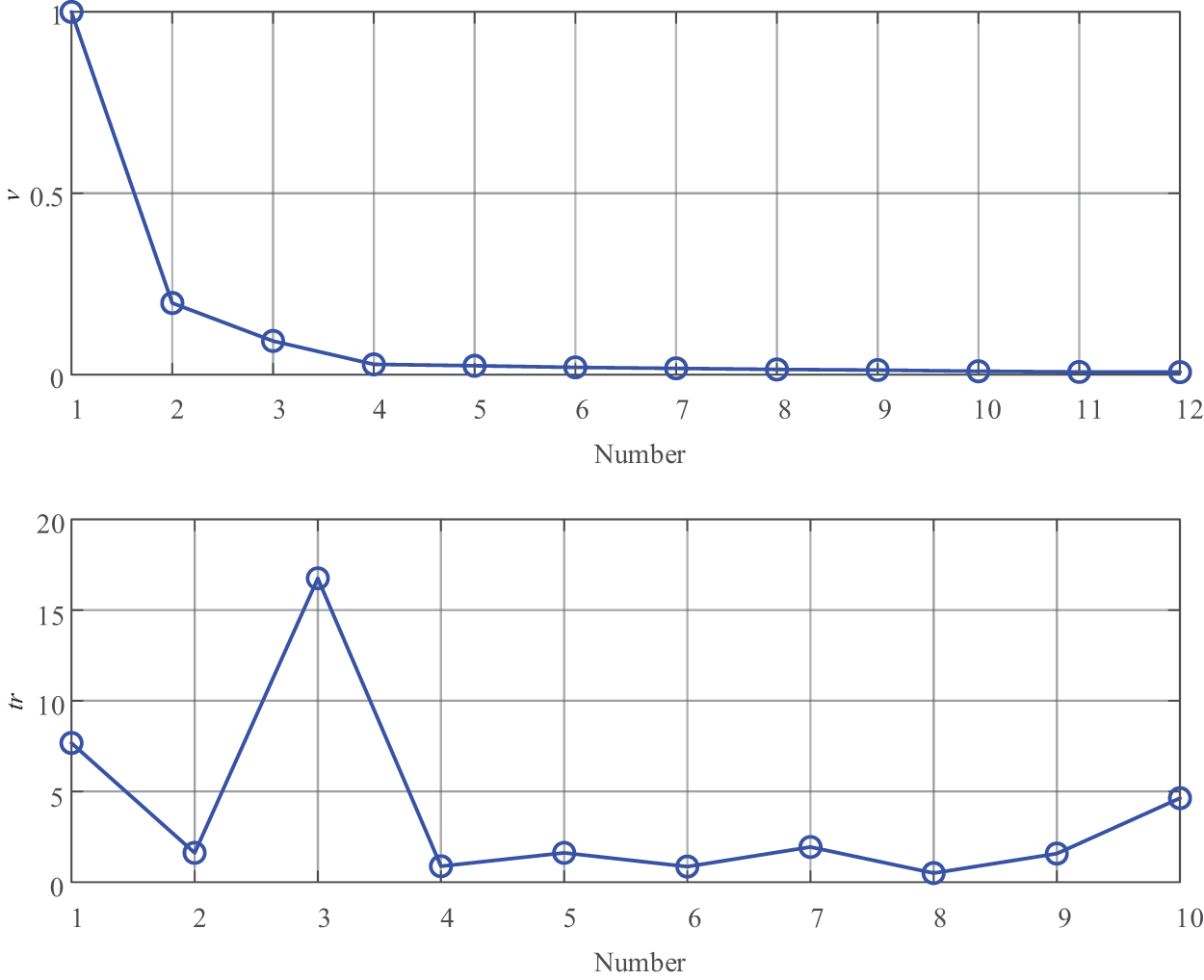
Figure 6: Slope trend of potential clustering centers

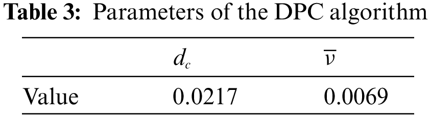
Remark 3: According to (10), the slope trend for data points can be calculated. There is a sharp decreasing tendency from tr3 to tr4 in Fig. 6, so the 3rd data point is the first non-clustering center and the first 2 data points are clustering centers.

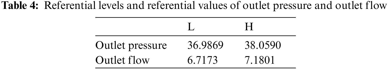
The components of each cluster center are arranged in ascending order and assigned to the referential values of indicators in the BRB. Since there are only two referential values for each indicator, the referential levels are described as Low (L) and High (H), referential values and referential levels of the two indicators are shown in Table 4.

Before performing inference, the matching degree of input needs to be calculated. For example,{(L,0.6775),(H,0.3225)} is the matching degree when x1=37.3326. The implication is that when the outlet pressure is 37.3326, the matching degree of outlet pressure relative to “L” is 0.6775, and relative to “H” is 0.3225. Other input information is converted in the same way.

4.3 Establishment of BRB

The k th rule is represented as follows:

Rk:If outlet pressure is A1k∧outlet flow is A2kthen health state is {(L,β1,k),{(M,β2,k),(H,β3,k)}with rule weight θkand indicator weight δ1,δ2(26)

where A1k and A2k represent the referential value for outlet pressure and outlet flow.

The health state is usually described as Low (L), Medium (M), and High (H), which is shown in Table 5.

All parameters of BRB are shown in Table 6, the indicator weight of outlet pressure and outlet flow are 1 and 0.6.

4.4 Testing of Health State Prediction Model

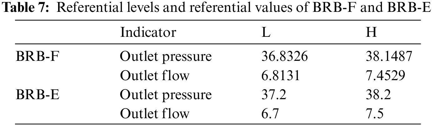
A BRB with the referential values given by the expert (BRB-E) and a BRB with the referential value determined based on fuzzy subtractive clustering (BRB-F) proposed in the literature [24] are constructed for comparison experiment, and the remaining parameters are the same as the BRB with the referential value determined based on the DPC (BRB-D), the referential values and referential levels of BRB-F and BRB-E are shown in Table 7.

The health state prediction results are obtained using BRB-D, BRB-F, and BRB-E fusion predicted data, respectively, and compared with the actual system. The comparison results are shown in Fig. 7, and the accuracy is shown in Table 8. By comparing the accuracy in Table 8, the BRB-D has the highest accuracy and is closer to the actual system, which proves the effectiveness of the proposed model.

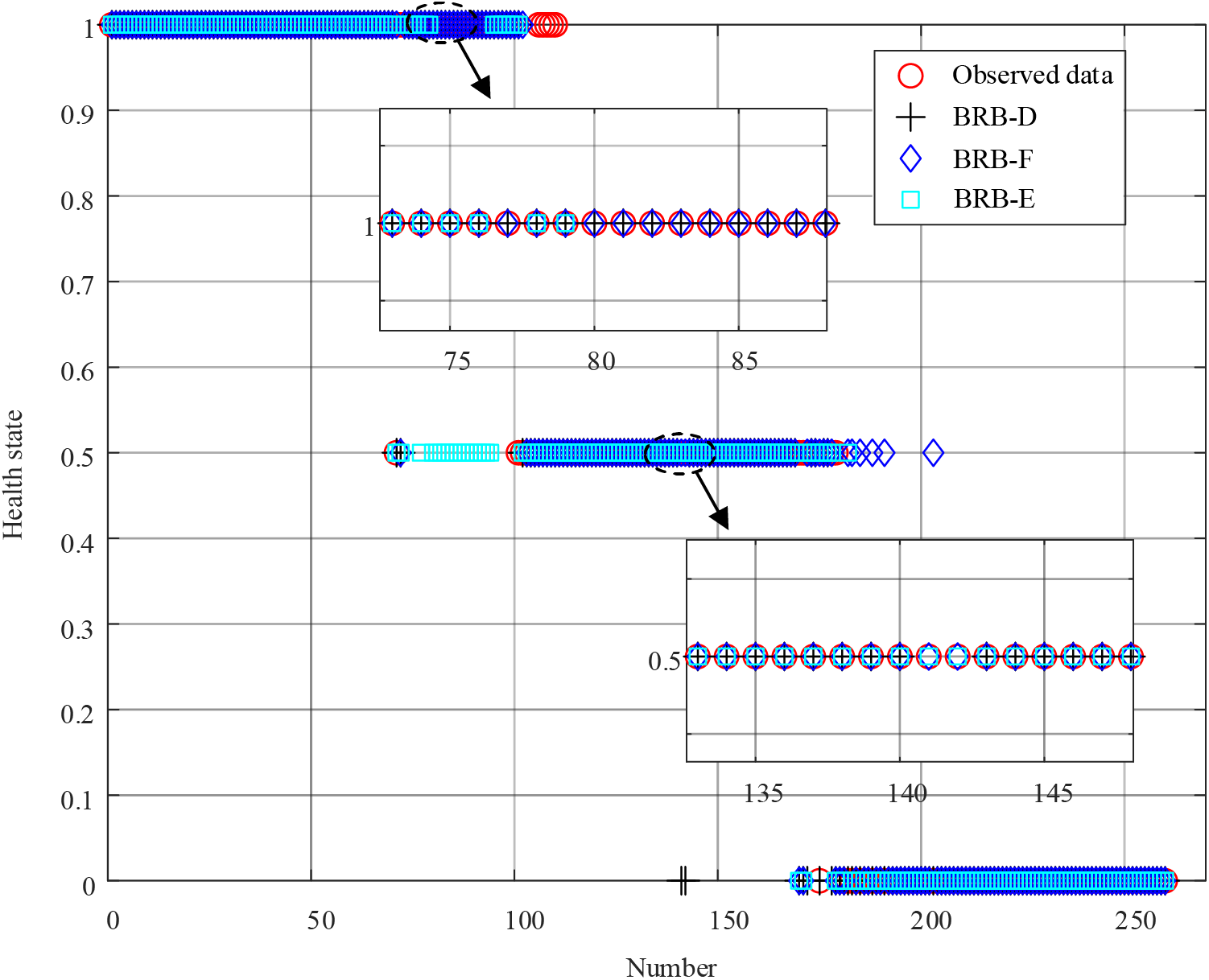
Figure 7: Comparative experiment

From Fig. 7, we can see that the predicted results of BRB-D, BRB-F, and BRB-E all have points that deviate from the actual system, while BRB-F and BRB-E have more. There are two main reasons for this. On the one hand, it is due to the unreasonable setting of the referential values. For example, for points 80 to 90, the actual system is “H”, while the prediction result of BRB-E is “M”. Since the referential values of outlet pressure and outlet flow about “H” in BRB-E is set high, resulting in the actual health state of H when both data are slightly below the referential values, while the prediction result obtained by BRB-E inference is “M”. Similarly, for points 190 to 200, the actual system is “L”, while the prediction result of BRB-F is “M”. Since the referential values of outlet pressure and outlet flow about “L” in BRB-F is set low, resulting in the actual health state of “L” when both data are slightly higher than the referential value, while the prediction result obtained by BRB-F inference is M. On the other hand, it is due to the deviation of the predicted values of outlet pressure and outlet flow from the observed data. For example, for points 141 and 142, the prediction results and belief distribution of the points are shown in Figs. 8 and 9. From Fig. 8, the predicted values of outlet pressure suddenly decrease at points 141 and 142 and are lower than the observed data. According to the calculation of (20)–(23), the belief degree of the health state increases with respect to “L” and decreases with respect to “M” in Fig. 9. Due to the error of the predicted value, the health state is “L” according to (25), while the actual system is “M”. Even if the predicted value of outlet flow increases at point 142, the health state is not maintained, which shows the influence of outlet pressure on the health state is more important than outlet flow, and the reasonableness of the indicator weight setting from the side.

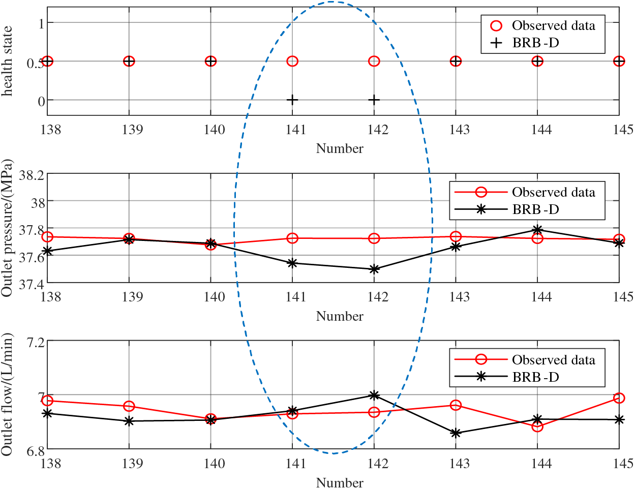
Figure 8: Prediction result of 141st and 142nd points

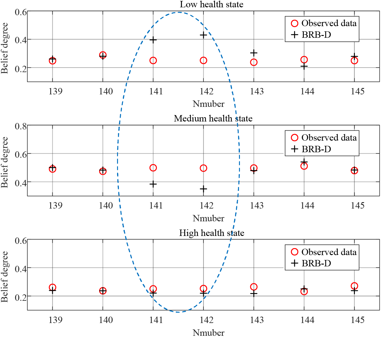
Figure 9: Belief distribution of 141st and 142nd points

5  Conclusion

In this paper, a prediction model based on BRB and LSTM is constructed to realize the prediction of the health state for complex systems. LSTM is used to provide the predicted values of indicators, and BRB is used to fuse the predicted values to obtain the health state. The proposed model can overcome the problem of a long-term dependence on indicators in traditional BRB prediction models and determine the referential values of indicators more rationally.

There are two main contributions in this paper. One is to combine LSTM and BRB to fuse multiple indicators for prediction, which reflects the health state more comprehensively. After embedding expert knowledge, the inference process of the model is transparent and clear, and the model parameters are easy to understand. Secondly, a determination method for the referential values of indicators is proposed to reflect the health state of the actual system division by selecting representative points, which offset the lack of expert knowledge. Through the comparative experiment, the proposed model has higher prediction accuracy than the existing BRB prediction model, which proves the effectiveness of the model.

In the case study, we assume that the prediction data obtained based on LSTM is completely reliable. However, the accuracy of the health state prediction results is reduced due to the deviation of the prediction values of indicators from the observed data. How to quantify the deviations and introduce the concept of reliability of prediction values of indicators to improve the quality of fused information and the prediction accuracy of BRB is the next research that needs to be carried out.

Acknowledgement: Thanks are due to Dr. Shuaiwen Tang and Dr. You Cao for the valuable discussion.

Funding Statement: This work was supported by the Natural Science Foundation of China under Grant 61833016 and 61873293, the Shaanxi Outstanding Youth Science Foundation under Grant 2020JC-34, and the Shaanxi Science and Technology Innovation Team under Grant 2022TD-24.

Author Contributions: Study conception and design: Yu Zhao and Zhijie Zhou; data collection: Yu Zhao; analysis and interpretation of results: Yu Zhao, Zhijie Zhou and Hongdong Fan; draft manuscript preparation: Yu Zhao, Xiaoxia Han, Jie Wang and Manlin Chen. All authors reviewed the results and approved the final version of the manuscript.

Availability of Data and Materials: The data are not publicly available due to the privacy of individuals that participated in the study.

Conflicts of Interest: The authors declare that they have no conflicts of interest to report regarding the present study.

References

1. J. Wang et al., “Maintenance strategy design for nuclear reactors safety systems using a constraint particle swarm evolutionary methodology,” Ann. Nucl. Energy., vol. 150, no. 1, pp. 107878, 2021. doi: 10.1016/j.anucene.2020.107878. [Google Scholar] [CrossRef]

2. C. H. Fleming, M. Spencer, J. Thomas, N. Leveson, and C. Wilkinson, “Safety assurance in NextGen and complex transportation systems,” Safety. Sci., vol. 55, no. 1, pp. 173–187, 2013. doi: 10.1016/j.ssci.2012.12.005. [Google Scholar] [CrossRef]

3. N. A. Nechval, G. Berzins, and K. N. Nechval, “Intelligent constructing exact statistical prediction and tolerance limits on future random quantities for prognostics and health management of complex systems,” Autom. Control. Comp. Sci., vol. 53, no. 6, pp. 532–549, 2019. doi: 10.3103/S0146411619060087. [Google Scholar] [CrossRef]

4. Y. A. Yucesan, A. Dourado, and F. A. C. Viana, “A survey of modeling for prognosis and health management of industrial equipment,” Adv. Eng. Inform., vol. 50, no. 1, pp. 101404, 2021. doi: 10.1016/j.aei.2021.101404. [Google Scholar] [CrossRef]

5. H. C. Vu, P. Do, B. Iung, and F. Peysson, “A case study on health prediction of an industrial diesel motor using particle filtering,” in Progn. Syst. Health Manage. Conf. (PHM), Harbin, China, 2017, pp. 1–7. [Google Scholar]

6. X. Li et al., “A data-driven approach for tool wear recognition and quantitative prediction based on radar map feature fusion,” Meas., vol. 185, no. 1, pp. 110072, 2021. doi: 10.1016/j.measurement.2021.110072. [Google Scholar] [CrossRef]

7. H. Ji et al., “State of health prediction model based on internal resistance,” Int. J. Energ. Res., vol. 44, no. 8, pp. 6502–6510, 2020. [Google Scholar]

8. A. Downey, Y. Lui, C. Hu, S. Laflamme, and S. Hu, “Physics-based prognostics of lithium-ion battery using non-linear least squares with dynamic bounds,” Reliab. Eng. Syst. Safe., vol. 182, no. 1, pp. 1–12, 2019. doi: 10.1016/j.ress.2018.09.018. [Google Scholar] [CrossRef]

9. N. Daroogheh, N. Meskin, and K. Khorasani, “An improved particle filtering-based approach for health prediction and prognosis of nonlinear systems,” J. Frankl. Inst., vol. 355, no. 8, pp. 3753–3794, 2018. doi: 10.1016/j.jfranklin.2018.02.023. [Google Scholar] [CrossRef]

10. R. Yuan, R. Chen, H. Li, W. Yang, and X. Li, “Dynamic reliability evaluation and life prediction of transmission system of multi-performance degraded wind turbine,” Comput. Model. Eng. Sci., vol. 135, no. 3, pp. 2331–2347, 2023. doi: 10.32604/cmes.2023.023788. [Google Scholar] [CrossRef]

11. H. Wu, A. Huang, and J. W. Sutherland, “Avoiding environmental consequences of equipment failure via an LSTM-based model for predictive maintenance,” Procedia Manuf., vol. 43, no. 1, pp. 666–673, 2020. doi: 10.1016/j.promfg.2020.02.131. [Google Scholar] [CrossRef]

12. Y. Li, X. Shan, W. Zhao, and G. Wang, “A LS-SVM based approach for turbine engines prognostics using sensor data,” in IEEE Int. Conf. Ind. Technol. (ICIT), Melbourne, Australia, 2019, pp. 983–987. [Google Scholar]

13. Y. Yang, J. Dong, C. Fang, P. Xie, and N. An, “FP-STE: A novel node failure prediction method based on spatio-temporal feature extraction in data centers,” Comput. Mode. Eng. Sci., vol. 123, no. 3, pp. 1015–1031, 2020. doi: 10.32604/cmes.2020.09404. [Google Scholar] [CrossRef]

14. M. Soleimani, F. Campean, and D. Neagu, “Integration of hidden markov modelling and bayesian network for fault detection and prediction of complex engineered systems,” Reliab. Eng. Syst. Safe., vol. 215, no. 1, pp. 107808, 2021. doi: 10.1016/j.ress.2021.107808. [Google Scholar] [CrossRef]

15. J. Xu, Z. Meng, and L. Xu, “Integrated system health management-based fuzzy on-board condition prediction for manned spacecraft avionics,” Qual. Reliab. Eng. Int., vol. 32, no. 1, pp. 153–165, 2016. doi: 10.1002/qre.1736. [Google Scholar] [CrossRef]

16. X. Liu, J. Zhu, C. Luo, L. Xiong, and Q. Pan, “Aero-engine health degradation estimation based on an underdetermined extended Kalman filter and convergence proof,” ISA Trans., vol. 53, no. 12, pp. 1–12, 2021. [Google Scholar]

17. Y. Zhang, L. Tu, Z. Xue, S. Li, L. Tian and X. Zheng, “Weight optimized unscented Kalman filter for degradation trend prediction of lithium-ion battery with error compensation strategy,” Energy, vol. 251, no. 15, pp. 123890, 2022. [Google Scholar]

18. Y. Liao, Y. Xiang, and M. Wang, “Health assessment and prognostics based on higher-order hidden semi-Markov models,” Nav. Res. Logist. (NRL), vol. 68, no. 2, pp. 259–276, 2021. [Google Scholar]

19. J. Pan, Y. Li, and P. Wu, “A predict method of water pump operating state based on improved particle swarm optimization of support vector machine,” J. Phys.: Conf. Ser., vol. 2160, no. 1, pp. 012056, 2022. doi: 10.1088/1742-6596/2160/1/012056. [Google Scholar] [CrossRef]

20. J. B. Yang, J. Liu, J. Wang, H. Sii, and H. Wang, “Belief rule-base inference methodology using the evidential reasoning Approach-RIMER,” IEEE. Trans. Syst., Man. Cybern–Part A: Syst. Hum., vol. 36, no. 2, pp. 266–285, 2006. doi: 10.1109/TSMCA.2005.851270. [Google Scholar] [CrossRef]

21. D. L. Xu et al., “Inference and learning methodology of belief-rule-based expert system for pipeline leak detection,” Expert. Syst. Appl., vol. 32, no. 1, pp. 103–113, 2007. doi: 10.1016/j.eswa.2005.11.015. [Google Scholar] [CrossRef]

22. G. L. Li, Z. J. Zhou, C. H. Hu, L. L. Chang, Z. G. Zhou and F. Zhao, “A new safety assessment model for complex system based on the conditional generalized minimum variance and the belief rule base,” Safety Sci., vol. 93, no. 1, pp. 108–120, 2017. doi: 10.1016/j.ssci.2016.11.011. [Google Scholar] [CrossRef]

23. X. J. Yin et al., “A double layer BRB model for health prognostics in complex electromechanical system,” IEEE Access, vol. 5, no. 1, pp. 23833–23847, 2017. doi: 10.1109/ACCESS.2017.2766086. [Google Scholar] [CrossRef]

24. G. Y. Hu et al., “Hidden behavior prediction of complex system based on time-delay belief rule base forecasting model,” Knowl.-Based Syst., vol. 203, no. 1, pp. 106147, 2020. doi: 10.1016/j.knosys.2020.106147. [Google Scholar] [CrossRef]

25. C. Cheng et al., “Health status prediction based on belief rule base for high-speed train running gear system,” IEEE Access, vol. 7, no. 1, pp. 4145–4159, 2019. [Google Scholar]

26. A. Ztürk and U. Zkaya, “Residual LSTM layered CNN for classification of gastrointestinal tract diseases,” J. Biomed. Inform., vol. 113, no. 1, pp. 103638, 2021. doi: 10.1016/j.jbi.2020.103638. [Google Scholar] [PubMed] [CrossRef]

27. F. Shahid, A. Zameer, and M. Muneeb, “A novel genetic LSTM model for wind power forecast,” Energy., vol. 22, no. 15, pp. 120069, 2021. doi: 10.1016/j.energy.2021.120069. [Google Scholar] [CrossRef]

28. A. Rodriguez and A. Laio, “Clustering by fast search and find of density peaks,” Sci., vol. 344, no. 1, pp. 1492–1496, 2014. doi: 10.1126/science.124207. [Google Scholar] [CrossRef]