A Hybrid Diffusion World Model for UAV Trajectory Forecasting and Collision Risk Estimation in Dense 3D Environments

1  Introduction

Unmanned aerial vehicles (UAVs) have evolved from remotely operated platforms into increasingly autonomous aerial systems used in logistics, infrastructure inspection, environmental monitoring, precision agriculture, disaster response, and urban air mobility. Among these applications, drone-based logistics and last-mile delivery have received substantial attention because UAVs can complement conventional ground transportation in time-sensitive missions and geographically constrained areas [1,2]. As UAV deployment expands from isolated operations to shared low-altitude airspace, autonomous navigation must address not only path efficiency but also dynamic obstacles, sensing uncertainty, aerodynamic disturbances, computational constraints, and real-time operational safety [3]. These challenges become particularly significant in dense three-dimensional environments.

In such environments, a UAV must maintain collision-free motion while simultaneously satisfying constraints related to velocity, acceleration, altitude, sensing range, control latency, and actuator capability. Conventional UAV navigation has primarily been addressed through search-based planning, evolutionary optimization, model-based control, and learning-assisted planning. Particle swarm optimization and genetic algorithms, for example, have been used to generate UAV trajectories under safety and motion constraints [4]. Control-oriented trajectory-planning methods have also been developed to improve trajectory feasibility under vehicle-dynamic limitations [5], while combinations of model predictive control (MPC) and reinforcement learning have been investigated for collision-aware UAV path planning [6]. Although these approaches can produce feasible or locally optimal trajectories, their effectiveness often depends on an accurate representation of the environment and its future evolution. In dense and dynamic scenes, however, a trajectory that is safe at the current timestep may become unsafe shortly afterward because of moving obstacles, wind disturbances, control variations, sensor noise, or partial observability. Consequently, navigation strategies based only on the current observation or on a single deterministic estimate may fail to identify hazardous events before they occur. Safe autonomous navigation therefore requires predictive reasoning, in which the UAV anticipates multiple possible future states and evaluates their safety before committing to a control action.

Trajectory prediction constitutes a central component of such predictive reasoning. Existing UAV trajectory-prediction methods range from classical filtering and mathematical models to machine-learning and deep-learning approaches [7]. The Kalman filter provides a fundamental framework for state estimation and prediction under noisy observations, but its conventional formulation relies on linear state-transition and observation assumptions [8]. Deep recurrent networks relax some of these assumptions by learning nonlinear temporal dependencies directly from trajectory data. Long short-term memory (LSTM) networks were introduced to capture long-range dependencies in sequential data [9], whereas gated recurrent unit (GRU) networks provide a more compact recurrent architecture with fewer gating mechanisms [10]. In UAV applications, recurrent LSTM models have been used with Automatic Dependent Surveillance-Broadcast information to predict trajectories in crowded low-altitude airspace [11]. GRU-based frameworks have demonstrated real-time and scalable UAV trajectory-forecasting capability [12], while velocity-enhanced GRU models have incorporated explicit motion information for three-dimensional prediction [13]. GRU networks have also been applied to UAV flight-path prediction for autonomous site assessment [14]. In addition, trajectory predictors have been combined with collision-risk classifiers in urban air-mobility applications, demonstrating that future-motion prediction can support early conflict warning [15]. Despite this progress, most recurrent UAV predictors generate adeterministic, single-modal point trajectory. Such deterministic predictions do not explicitly represent the multimodal nature of future motion. Given the same state and observation history, several future trajectories may remain plausible because of uncertain obstacle behavior, depth-measurement errors, wind disturbances, and variations in the executed control action. A single forecast may therefore conceal low-probability but safety-critical outcomes. Moreover, evaluating a trajectory predictor only through displacement metrics, such as average displacement error or final displacement error, does not directly determine whether the predicted trajectory remains collision-free or maintains sufficient obstacle clearance. These limitations motivate a transition from predicting only where a UAV may move toward jointly predicting how its future motion may evolve and whether that motion is likely to remain safe.

World models provide a suitable conceptual foundation for this transition. A world model learns an internal representation of environment dynamics and uses this representation to imagine possible future states before actions are executed. Early recurrent world models demonstrated that learned generative dynamics can support policy evolution through imagined rollouts [16]. More recent research has shown that world models can support decision-making across diverse control tasks by learning predictive representations of the environment [17]. For UAV navigation, a world model can therefore operate as an intermediate predictive layer between multimodal perception and downstream control, allowing the system to assess the potential consequences of candidate motions under uncertain environmental conditions. To effectively implement the multimodal generative capability required by such world models, diffusion models have emerged as a powerful family of generative models for learning complex and multimodal probability distributions. Denoising diffusion probabilistic models formulate generation through a progressive noising and denoising procedure [18], while score-based generative modeling provides a continuous-time stochastic differential-equation interpretation of this process [19]. Diffusion models have demonstrated strong capability in modeling high-dimensional and multimodal data distributions [20]. Beyond image synthesis, they have been extended to trajectory generation and robotic decision-making. Diffuser formulates planning as conditional denoising over future trajectories [21], whereas Diffusion Policy models visuomotor control as an iterative action-denoising process [22]. These properties make diffusion models particularly relevant to UAV trajectory forecasting because multiple stochastic rollouts can be generated from the same historical context rather than restricting prediction to a single deterministic future.

Nevertheless, generative trajectory prediction alone does not guarantee safe closed-loop behavior. A learned predictor may become inaccurate under distribution shifts, unobserved obstacle configurations, or disturbance levels that differ from those represented in the training data. Even when a predicted trajectory is accurate, the prediction mechanism does not inherently prevent a downstream controller from selecting an unsafe action. Control-theoretic safety mechanisms therefore provide an important complementary layer. Control Barrier Functions (CBFs) define forward-invariant safe sets and formulate constraints that prevent a controlled system from entering unsafe regions [23]. In UAV applications, collision-cone CBFs have been developed for obstacle avoidance in dynamic environments [24]. Higher-order CBFs have been applied to collision-avoidance guidance in multi-UAV pursuit-evasion scenarios [25], while CBF-based runtime-assurance methods have been studied for fixed-wing collision avoidance and geofencing [26]. Collision-cone CBF formulations have also been investigated for real-time fixed-wing UAV safety under static and dynamic obstacles [27]. More recent studies integrate CBF constraints with MPC-based UAV obstacle avoidance [28] or improve collision-cone formulations for dynamic-obstacle scenarios [29]. A related research direction combines generative planning with explicit safety constraints. Diffusion-based conditional planning has been integrated with control barrier and Lyapunov functions for dynamic robot environments [30]. SafeDiffuser incorporates safety constraints into diffusion-based planning [31], while flow-matching approaches have similarly been combined with CBFs for safe robot motion planning [32]. Dynamic high-order CBFs have also been integrated with diffusion-based planning for safety-critical trajectory generation [33]. These studies demonstrate the potential of coupling generative future modeling with explicit safety reasoning.

Despite the progress in UAV trajectory prediction, diffusion-based planning, and control-theoretic safety filtering, several limitations remain. First, existing UAV trajectory predictors predominantly generate deterministic trajectories and therefore do not explicitly represent multiple plausible future outcomes caused by sensing uncertainty, disturbances, and dynamic-obstacle motion. Second, trajectory prediction and collision-risk estimation are often treated as separate tasks; consequently, a low trajectory-displacement error does not necessarily correspond to reliable prediction of collision, near-miss, or unsafe-clearance events. Third, existing diffusion-based planning studies are largely developed for general robotic motion planning, while comparatively limited attention has been given to task-specific diffusion world models that jointly use UAV state-action history, depth observations, and safety context to forecast future three-dimensional UAV motion. Fourth, only limited work has investigated a unified predictive interface that produces multimodal trajectory rollouts together with horizon-wise collision probability, near-miss probability, and minimum obstacle-distance estimates for downstream safety filtering. Finally, conventional safety strategies frequently rely on predefined safety margins and do not explicitly adapt these margins according to predicted trajectory dispersion, relative closing speed, and collision likelihood.

To address these gaps, this paper proposes a hybrid diffusion world model for short-horizon UAV trajectory forecasting and predictive collision-risk estimation in dense three-dimensional environments. The framework conditions its predictions on historical UAV states, executed control actions, the current depth observation, and the current safety context. Instead of reconstructing complete future RGB images or depth maps, the model learns a conditional distribution over future relative UAV position and velocity during a 1.0 s prediction horizon. A conditional diffusion branch generates plausible future motion rollouts, while dedicated supervised risk heads estimate horizon-wise collision probability, near-miss probability, and minimum obstacle distance. This design concentrates the learned world model on motion and safety variables that are directly relevant to predictive collision avoidance. Multiple diffusion rollouts can additionally be used to characterize future-trajectory dispersion and sampled collision likelihood. These outputs define an interface through which a downstream safety supervisor may adjust its minimum safety margin according to predicted uncertainty, relative closing speed, and collision risk. The learned predictive representation is evaluated first in open-loop forecasting and risk-estimation settings and subsequently in closed-loop experiments that assess whether model-generated future trajectories and risk estimates can support safety-aware action selection. Oracle simulator rollouts, where retained, are used only as a reference upper bound rather than as the principal decision mechanism. To address the aforementioned research gaps, this study makes the following main contributions:

1.   We propose a joint diffusion-based world model for UAV navigation that simultaneously represents multiple plausible future trajectories and predicts horizon-wise safety variables, including collision probability, near-miss probability, and minimum obstacle distance. Unlike deterministic recurrent predictors that provide a single future trajectory, the proposed formulation models future motion as a conditional distribution and couples this multimodal representation with explicit probabilistic risk estimation.

2.   We introduce a unified trajectory–risk learning formulation in which historical UAV state–action information, depth observations, and safety-context variables are jointly exploited for predictive safety modeling. The resulting architecture enables the same predictive representation to support both future-motion generation and calibrated collision-risk estimation. This design is further examined through risk-only, trajectory-only, deterministic, no-depth, and no-safety-context ablations to quantify the contribution and trade-offs of each component.

3.   We establish a reviewer-aligned experimental protocol for statistically rigorous comparison across recurrent, deterministic, generative, and risk-only models. All model families use the same episode-level data partitions, preprocessing pipeline, historical context, prediction horizon, validation-based threshold selection, and five independent training seeds. Evaluation is performed on the complete test partition using episode-level bootstrap confidence intervals, multimodal best-of-K metrics, trajectory diversity, Brier score, expected calibration error, and reliability analysis.

4.   We evaluate the proposed model under both distribution shift and end-to-end closed-loop integration. A dedicated OOD test suite is used to analyze failure modes caused by unseen obstacle density, size, and motion characteristics, while a paired closed-loop stress test evaluates learned-model action selection against nominal control and simulator-based rollout references. The results reveal a practical speed–safety trade-off: learned diffusion rollouts provide substantially lower planning latency than simulator rollouts, while safety improvements remain scenario-dependent under challenging OOD conditions.

2  Related Work

2.1 UAV Navigation and Trajectory Prediction in 3D Environments

UAV navigation in three-dimensional environments is an important problem in autonomous aerial systems, especially when UAVs are deployed in scenarios involving numerous obstacles, narrow spaces, high vehicle density, or uncertain sensing conditions. Unlike navigation on a two-dimensional plane, UAVs operate in three-dimensional space; therefore, their motion state commonly includes position, velocity, heading, acceleration, and kinematic or dynamic constraints related to the vehicle’s maneuverability [1,2]. In essence, the UAV navigation problem can be viewed as a combination of trajectory planning, environmental perception, future-state prediction, and safety-aware control. A UAV needs to construct or receive environmental information from sensors, maps, or simulations, and then generate a sequence of actions that enables the vehicle to move from its current state to the desired goal. However, in dense 3D environments, a flight path that is optimal in terms of distance is not necessarily safe, because factors such as dynamic obstacles, sensor noise, localization errors, control delay, and dynamic limitations can increase collision risk [3,4]. UAV trajectory prediction plays a central role in safe navigation. Instead of reacting only to the current state, the system needs to predict the future evolution of the UAV over a short time window, such as several steps or several seconds ahead. This prediction may include future position, velocity, minimum distance to obstacles, near-miss likelihood, and collision probability. Recent studies show that deep learning can support trajectory prediction and collision-risk estimation in UAV or Urban Air Mobility scenarios, especially when motion data are sequential and influenced by spatial context [7,15].

2.2 Traditional Time-Series Data-Driven Approaches

Traditional time-series prediction methods are generally based on the assumption that the future state of a system can be inferred from its current state and a set of past observations. In the UAV problem, timeseries data may include position, velocity, acceleration, heading, distance to obstacles, and other variables related to the environmental state [34]. One classical foundation of state prediction is the Kalman filter, in which the hidden state of a dynamic system is estimated through a state-transition model and noisy observations [8]. Kalman-filter-based variants are often suitable for systems with linear or near-linear models, but they may face limitations when the UAV environment contains strong nonlinearities, complex obstacles, and rapidly changing control behaviors. When motion data are nonlinear and involve long-term dependencies, deep time-series models are increasingly used, especially recurrent neural networks (RNNs), long shortterm memory (LSTM), and gated recurrent unit (GRU) networks. LSTM was developed to reduce the vanishing-gradient problem in long-sequence learning, thereby enabling the model to retain information across multiple timesteps [9]. GRU is a simpler variant with a gated mechanism, often requiring fewer parameters than LSTM while still maintaining the ability to learn temporal dependencies [10]. In UAV trajectory prediction, these models can learn the relationship between past motion and future position without fully modeling the UAV’s dynamic equations. Many recent studies have applied LSTM and GRU models to UAV trajectory prediction. Zhang et al. used a recurrent LSTM model based on ADS-B information to predict UAV trajectories, demonstrating the ability to exploit historical data in aerial motion prediction [11]. Other studies have developed GRU-based prediction frameworks to improve real-time processing, accuracy, and scalability in UAV environments [12]. VECTOR further extends this direction by enhancing GRU networks with velocity information to improve real-time 3D UAV trajectory prediction [13]. In addition, recent studies have also used GRU for UAV flight-path prediction in the context of autonomous site assessment [14]. Although LSTM and GRU models are effective for trajectory prediction, they commonly produce a point trajectory or a deterministic sequence of predictions. This may be insufficient in highly uncertain 3D environments, where the same current state can lead to multiple plausible futures. Therefore, traditional time-series models may need to be combined with uncertainty estimation, multimodal prediction, or safety-filtering mechanisms to ensure that predicted trajectories are meaningful for real-world control. In this context, world models and generative models such as diffusion models have begun to receive increasing attention because they can learn a distribution over future outcomes instead of predicting only a single result. A world model allows an agent to simulate future evolution in a latent space or state space, thereby supporting planning and control [17]. Diffusion models and score-based generative modeling provide a foundation for generating data through a denoising process, which may be suitable for multimodal time-series prediction problems [18,19]. Therefore, compared with traditional GRU/LSTM models, a diffusion world model can be viewed as an extended direction for modeling the future as a distribution, making it suitable for UAV problems involving high risk and uncertainty.

2.3 UAV Trajectory Prediction and Collision Avoidance

Recent UAV navigation studies increasingly use learning-based methods to predict future motion instead of relying only on reactive obstacle avoidance. Shukla et al. review conventional, machine-learning, and deep-learning approaches for UAV trajectory prediction [7]. Recurrent neural networks are particularly common because UAV trajectories are naturally represented as temporal sequences. Yoon et al. propose a GRU-based framework for real-time UAV trajectory forecasting and discuss its relevance to collision avoidance, mission planning, and anti-drone systems [12]. Nacar et al. introduce a velocity-enhanced GRU network for real-time 3D UAV trajectory prediction using historical position and velocity information [13]. Zhang et al. propose a recurrent LSTM-based UAV trajectory-prediction method using ADS-B information for crowded low-altitude airspace [11]. Kim et al. combine LSTM Attention trajectory prediction with collision-risk classification for urban air mobility [15]. These studies show that short-horizon prediction can support early conflict warning. However, most recurrent methods generate deterministic point forecasts and do not explicitly represent multiple plausible futures under sensing uncertainty or disturbances. Collision avoidance can also be enforced through optimization-based safety filters. Liu et al. develop a controloriented trajectory planning method under UAV motion constraints [5]. Tayal et al. introduce collisioncone Control Barrier Functions (CBFs), which modify control commands through quadratic programming to avoid static and moving obstacles [24]. However, conventional safety constraints commonly use predefined margins and do not adapt the minimum safe distance according to predicted uncertainty, relative closing speed, and collision probability.

2.4 Control-Theoretic Collision Risk Assessment and Safety Filtering

Recent UAV studies show that navigation in three-dimensional environments is increasingly being expanded into a framework that combines prediction, risk assessment, and safety-aware control. Recent surveys emphasize that UAV trajectory prediction should be extended from position prediction to the prediction of risk, uncertainty, and interaction with the environment [7]. Kim et al. also proposed a deeplearning framework for Urban Air Mobility that combines trajectory prediction and collision-risk assessment, showing that the current research logic is shifting from “predict where the UAV will go” to “predict whether the future trajectory is safe” [15]. From a modeling perspective, world models provide a suitable foundation for building future-prediction capability in autonomous agents. Instead of directly learning only control actions, a world model learns an internal representation of the environment and simulates the future evolution of system states. Hafner et al. showed that world models can support agents in mastering diverse control tasks by learning the dynamics of the environment [17]. For UAVs, this logic is important because the system needs to “imagine” possible future trajectories before selecting a control action. When combined with flight-state data and 3D environmental information, a world model can serve as a predictive layer that enables the UAV to evaluate the short-term consequences of its actions. Nevertheless, machine-learning models or generative models do not automatically guarantee that their output actions are always safe. This is why safety-aware control methods based on Control Barrier Functions (CBFs) are used as an independent protective layer. A CBF defines a safe set of states and designs control constraints so that the system does not leave that safe set [23]. In UAV applications, Tayal et al. applied CBFs with a collision-cone formulation for obstacle avoidance during flight [24]. Lv et al. proposed a collision-avoidance guidance strategy for multiple fixed-wing UAVs based on High-Order Control Barrier Functions, in which CBF constraints are integrated into an optimization problem to maintain safe distances among UAVs [25]. Molnar et al. extended this direction to collision avoidance and geofencing for fixed-wing aircraft, using CBFs as a safety filter in a run-time assurance system [26]. Agarwal et al. further investigated collision-cone CBFs for real-time safety of fixed-wing UAVs in environments with static and dynamic obstacles [27]. Based on these research directions, the theoretical framework of this study can be formulated as follows. First, a UAV requires a trajectory-prediction model to identify possible future states in a 3D environment [7,11–15]. Second, because UAV environments involve high uncertainty, the prediction model should be extended from position prediction to the prediction of safety indicators, including minimum distance, near-miss events, and collision risk. This provides the basis for using a diffusion world model as a safety-oriented prediction module [16–22,30–32]. Third, because a datadriven prediction model does not inherently guarantee control safety, this study additionally evaluates safety-filtering strategies in closed-loop settings to analyze the effects of safety constraints on collision frequency and safe clearance [23–27]. Accordingly, this study is built on a three-layer logic: trajectory prediction using a diffusion world model, risk assessment through collision, near-miss, and minimumdistance prediction, and closed-loop verification with fixed and adaptive safety strategies in dense 3D UAV environments.

3  Methodology

The proposed framework consists of three main stages: simulation-based dataset generation, collision-risk annotation, and diffusion-based future state prediction. First, diverse UAV navigation episodes are generated under varying obstacle configurations, controller behaviors, sensing uncertainties, and aerodynamic disturbances. Second, synchronized trajectories are annotated with instantaneous and future collision-risk labels. Finally, the resulting multimodal sequences are used to train a diffusion-world model for future-state rollout and collision-aware trajectory evaluation.

3.1 Simulation-Based Dataset Generation

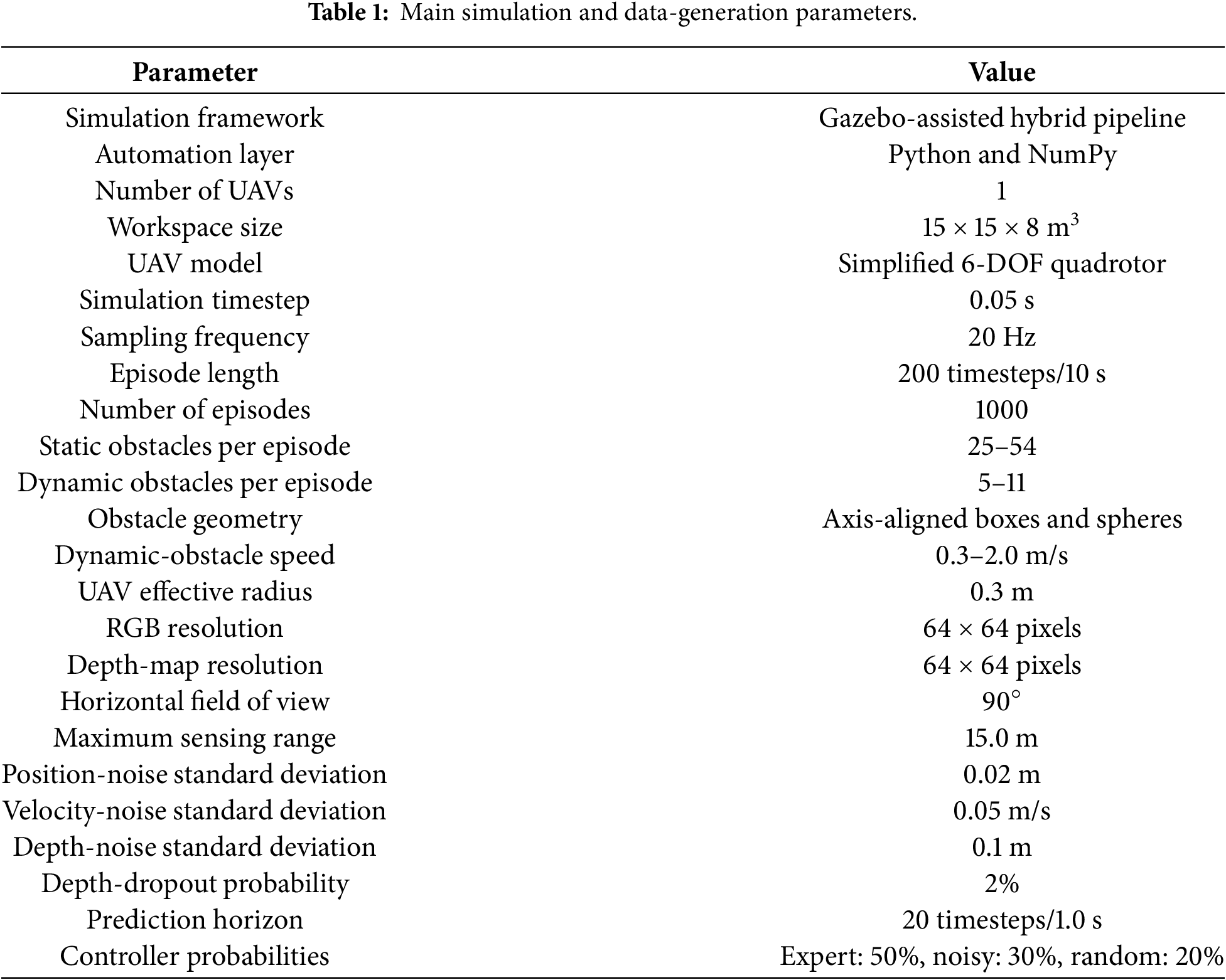
A Gazebo-assisted hybrid simulation pipeline is developed to generate a task-specific dataset for predictive collision avoidance. Gazebo is used to construct the base three-dimensional UAV environment and execute representative navigation scenarios. A Python/NumPy orchestration layer is employed to automate procedural scenario randomization, temporal sampling, disturbance injection, geometry-based observation synthesis, synchronized data recording, and risk-label generation. This hybrid design enables the systematic generation of safety-critical trajectories without exposing physical UAV hardware to collision risks. The simulated workspace has a size of 15×15×8 m3. For each episode, the obstacle configuration is regenerated to increase scene diversity. The environment contains both static and dynamic obstacles, represented by axis-aligned boxes and spheres. The number of static obstacles varies from 25 to 54, while the number of dynamic obstacles varies from 5 to 11. Dynamic obstacles move along linear trajectories with randomly sampled speeds ranging from 0.3 to 2.0 m/s and reverse their direction when reaching the environment boundaries. The initial UAV position is sampled from a collision-free region with a minimum clearance of 2.0 m, whereas each navigation goal is generated at least 5.0 m away from the current UAV position. The UAV is represented by a simplified six-degree-of-freedom quadrotor model. Its state vector is defined as

st=[xt,yt,zt,qw,t,qx,t,qy,t,qz,t,vx,t,vy,t,vz,t,ωx,t,ωy,t,ωz,t]⊤.(1)

where (xt,yt,zt) denotes the UAV position, (qw,t,qx,t,qy,t,qz,t) is the quaternion-based orientation, (vx,t,vy,t,vz,t) is the linear velocity, and (ωx,t,ωy,t,ωz,t) is the angular velocity. The control vector is written as

ut=[Tt,τx,t,τy,t,τz,t]⊤,(2)

where Tt is the total thrust and (τx,t,τy,t,τz,t) are the body torques. The motion model incorporates gravitational force, aerodynamic drag, motor lag, stochastic process noise, and time-varying wind disturbances. Each episode consists of 200 timesteps with a sampling interval of 0.05 s, corresponding to a sampling frequency of 20 Hz and an episode duration of 10 s. To improve state-space coverage, three controller modes are used during data generation: expert, noisy, and random controllers. Their nominal sampling probabilities are set to 50%, 30%, and 20%, respectively. The controller mixture increases exposure to nominal trajectories, near-miss situations, and collision-prone behaviors. At each timestep, the pipeline records the UAV state, control action, and obstacle configuration. Synchronized RGB images, depth maps, point clouds, and occupancy grids are additionally generated to represent the spatial structure of the surrounding environment. Both RGB images and depth maps have a resolution of 64×64 pixels. The horizontal camera field of view is 90∘, and the maximum sensing range is 15 m. To represent uncertain sensing conditions, Gaussian noise is introduced into UAV position, velocity, and depth observations. A random depth dropout probability of 2% is additionally applied. The main simulation and data-generation parameters are summarized in Table 1.

3.2 Collision-Risk Annotation

Let dt denote the distance from the UAV center to the surface of the nearest obstacle at timestep t, and let rUAV=0.3 m denote the effective UAV radius. The instantaneous collision label is defined as

ct={1,dt≤rUAV,0,dt>rUAV.(3)

A near-miss label is assigned when the UAV does not collide with an obstacle but the remaining clearance is smaller than the threshold δnm=1.0 m:

nt=I[ct=0∧(dt−rUAV)<δnm].(4)

In addition to the instantaneous labels, the dataset stores future collision indicators and future minimum distances over a prediction horizon of H=20 timesteps. The future-collision vector is defined as

ct+=[ct+1,ct+2,…,ct+H]⊤.(5)

A trajectory-safe label is assigned when no collision occurs within the prediction horizon:

ytsafe=I[∑h=1Hct+h=0].(6)

This annotation strategy enables the model to estimate emerging risk before a collision is physically observed.

3.3 Dataset Composition and Descriptive Statistics

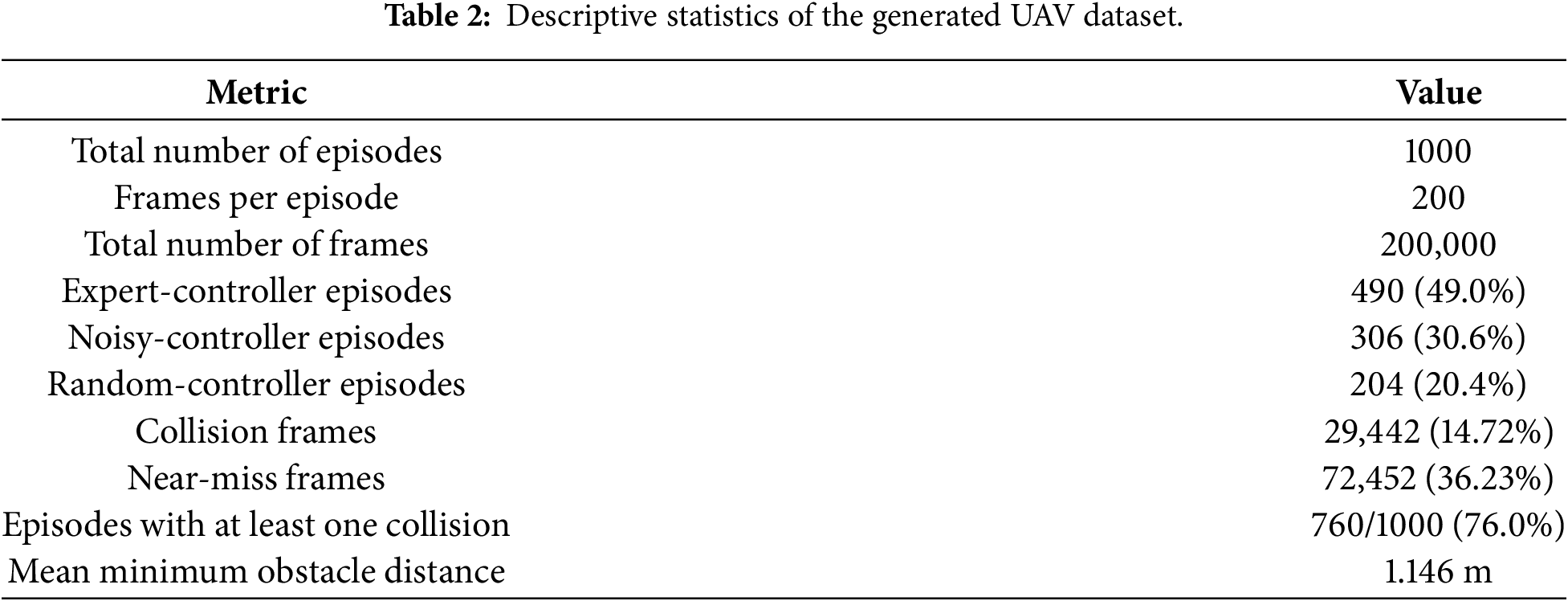
The resulting dataset contains 1000 episodes and 200,000 temporally synchronized frames. The realized controller distribution consists of 490 expert-controller episodes, 306 noisy-controller episodes, and 204 random-controller episodes. The generated trajectories cover nominal flight, near-miss situations, and collision-prone behaviors. As summarized in Table 2, collision frames account for 14.72% of all samples, while near-miss frames account for 36.23%. In addition, 760 out of 1000 episodes contain at least one collision event. The mean minimum distance to the nearest obstacle is 1.146 m. The substantial proportion of near-miss samples is particularly relevant to predictive collision avoidance because these frames characterize the transition region between safe navigation and physical contact.

The use of a task-specific synthetic dataset offers three practical advantages. First, it enables controlled variation of obstacle density, obstacle motion, controller behavior, sensing noise, and aerodynamic disturbances. Second, hazardous and failure-prone trajectories can be generated without risking physical UAV hardware. Third, synchronized future-risk labels can be computed directly from the simulated trajectories, which is essential for training a predictive world model.

3.4 Episode-Level Partition and OOD Test Suite

The 1000 in-distribution (ID) episodes are partitioned exclusively at the episode level into 697 training episodes, 148 validation episodes, and 155 test episodes. No episode identifier is shared across these subsets. The same immutable partition files are used by every baseline, ablation model, random seed, and evaluation procedure. This prevents temporal leakage that would otherwise arise if overlapping windows from the same episode were distributed across different subsets. In addition to the ID dataset, a separate OOD test suite contains 300 episodes and is not used for training, hyperparameter selection, normalization, probability-threshold selection, or checkpoint selection. The suite is divided into three 100-episode profiles: sparse environments with faster dynamic obstacles, dense environments containing smaller obstacles, and environments containing substantially larger obstacles. The resulting dataset hierarchy is illustrated in Fig. 1, which separates the immutable ID train/validation/test partitions from the independent OOD test suite. This organization makes the role of each subset explicit and prevents the OOD profiles from influencing model fitting or model selection.

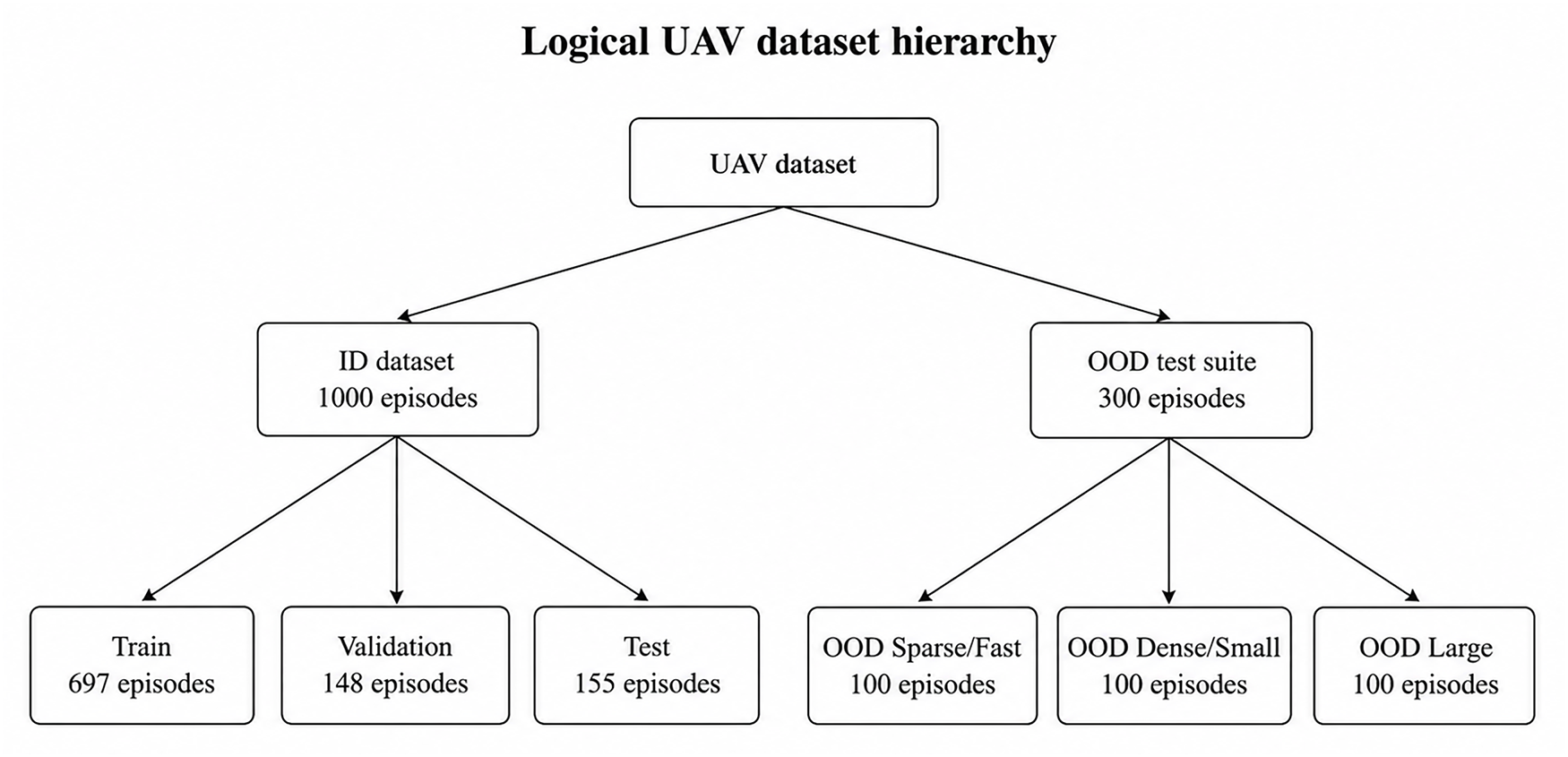
Figure 1: Logical organization of the in-distribution dataset and the independent OOD test suite. The ID dataset is split exclusively at the episode level, while the three OOD profiles are reserved for post-training generalization evaluation.

Table 3 summarizes the controlled distribution shifts used to define the ID and OOD scenario profiles. Relative to the ID setting, OOD Sparse/Fast increases dynamic-obstacle speed and dynamic-obstacle count, OOD Dense/Small substantially increases obstacle density while reducing obstacle size, and OOD Large introduces obstacle sizes outside the ID range. These controlled shifts are designed to isolate different forms of geometric and dynamic distribution change.

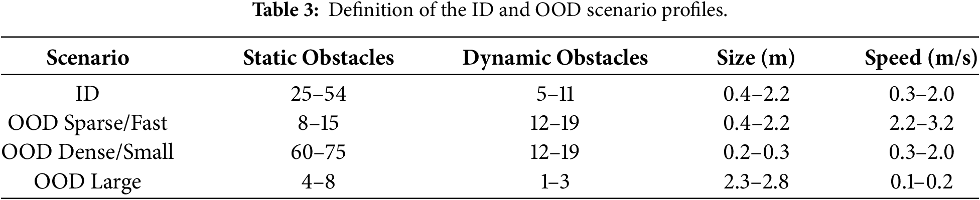
Fig. 2 provides qualitative examples from the three OOD profiles. The normal, near-miss, and collision cases show that the dataset contains not only different obstacle distributions but also safety outcomes spanning routine navigation, reduced-clearance interactions, and physical-contact events. The paired RGB, depth, and top-down views provide complementary visual evidence of scene appearance, sensed obstacle proximity, and trajectory-level behavior.

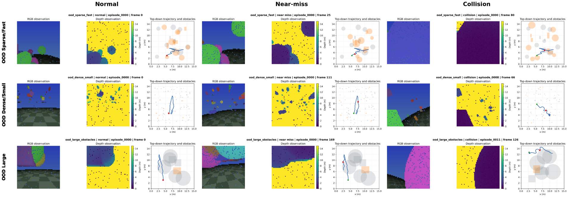
Figure 2: Representative samples from the OOD UAV test suite. Rows correspond to the OOD Sparse/Fast, OOD Dense/Small, and OOD Large scenario profiles, while columns show normal, near-miss, and collision cases. Each panel contains the RGB observation, metric depth observation, and top-down UAV trajectory with static and dynamic obstacles.

3.5 Proposed Hybrid Diffusion World Model

The proposed model is designed as a compact predictive world model for short-horizon UAV trajectory forecasting and probabilistic safety estimation. Rather than reconstructing future RGB or depth observations, it models future relative UAV motion and associated safety variables. The architecture combines (i) a numerical encoder for historical state-action information and safety context, (ii) a depth encoder for the current spatial observation, (iii) a conditional trajectory-diffusion branch, and (iv) supervised heads for collision, near-miss, and minimum-distance prediction.

3.5.1 Input and Target Representation

At timestep t, the model receives a historical context window of W=10 timesteps. Since the simulation frequency is 20 Hz, the historical context represents the previous 0.5 s of UAV motion. The numerical conditioning vector is defined as

z=[s~t−W:t−1,ut−W:t−1,rt].(7)

where s~t−W:t−1 is the stored UAV-state history, ut−W:t−1 is the executed action history, and rt is the current safety context. The stored state representation used by the learning module augments the physical state defined above with roll, pitch, and yaw:

s~t=[xt,yt,zt,qw,t,qx,t,qy,t,qz,t,ϕt,θt,ψt,vx,t,vy,t,vz,t,ωx,t,ωy,t,ωz,t]⊤.(8)

The safety-context vector is

rt=[ct,nt,dtmin]⊤,(9)

where ct is the instantaneous collision label, nt is the instantaneous near-miss label, and dtmin is the minimum distance to the nearest obstacle surface. Each stored state contains 16 variables, while the action representation follows the control schema stored in the released dataset. The current safety-context vector contains three variables. The exact action-channel definition is kept identical across the proposed model and all matched baselines. The model additionally receives the current depth map Dt. The original 64×64 depth observation is downsampled to 32×32, clipped to the sensing range, normalized to [0,1], and flattened into a 1024-dimensional vector. A key design choice is to forecast future motion relative to the current UAV state rather than predicting absolute future coordinates. For each prediction step h∈{1,…,H},

Δpt+h=pt+h−pt,Δvt+h=vt+h−vt.(10)

The clean trajectory target is

y0=[Δpt+1,Δvt+1,…,Δpt+H,Δvt+H].(11)

With H=20, corresponding to a prediction horizon of 1.0 s, the target dimension is dim⁡(y0)=6H=6×20=120. The relative representation reduces sensitivity to absolute workspace coordinates and mitigates trajectory drift during reverse-diffusion sampling. The collision, near-miss, and safe-trajectory labels are defined based on the distance between the UAV and the nearest obstacle. This distance-based labeling follows the common logic of trajectory prediction and collision-risk assessment, where future states are evaluated not only by positional accuracy but also by whether they violate a safety region around the vehicle [7,15]. Specifically, an instantaneous collision is assigned when the nearest-obstacle distance is smaller than or equal to the effective UAV radius. A near-miss label is assigned when the UAV has not collided but its remaining clearance is below a predefined near-miss threshold. Similar safety-distance reasoning is also consistent with recent UAV collision-avoidance studies using control barrier functions and collision-cone constraints, where safety is formulated by preventing the vehicle state or relative motion from entering unsafe regions [23–27]. Therefore, the future collision vector and safe-trajectory label are used in this study to convert geometric proximity information into supervised risk labels over the prediction horizon.

3.5.2 Conditional Trajectory Diffusion

The numerical conditioning vector and current depth observation are processed independently by multilayer perceptrons. The numerical encoder maps z into a 384-dimensional representation, while the depth encoder maps Dt into a 128-dimensional representation. A sinusoidal embedding represents the diffusion timestep. Following denoising diffusion and score-based generative modeling principles [18,19], Gaussian noise is added to the clean future trajectory during training:

yτ=α¯τy0+1−α¯τε,ε ∼𝒩(0,I),(12)

where τ is the diffusion timestep and α¯τ is the cumulative product of the noise schedule. The denoising network receives the noisy trajectory, encoded numerical context, encoded depth observation, and diffusion-time embedding. It predicts the added noise:

ε^= εθ(yτ,τ,z,Dt).(13)

The estimated clean trajectory is recovered as

y^0=yτ−1−α¯τε^α¯τ.(14)

Similar to conditional diffusion models for trajectory generation and robot behavior synthesis [21,22,30], the denoising network receives the noisy trajectory, encoded numerical context, encoded depth observation, and diffusion-time embedding.

3.5.3 Supervised Safety-Risk Heads

Continuous trajectory generation and safety-risk estimation are separated because trajectory variables, binary risk indicators, and obstacle distances have different statistical properties. The predicted clean trajectory is combined with a shared risk-context representation. Three dedicated heads estimate the future safety variables:

c^t+=σ(fcol(y^0,z,Dt)),n^t+=σ(fnm(y^0,z,Dt)),d^t+=ReLU(fmd(y^0,z,Dt)),(15)

where c^t+∈[0,1]H contains future collision probabilities, n^t+∈[0,1]H contains future near-miss probabilities, and d^t+∈R≥0H contains predicted minimum distances. Each risk head contains two hidden layers with 256 and 128 units, followed by an output layer with H=20 values.

3.5.4 Multi-Task Training Objective

The proposed model is trained using the weighted multi-task objective

ℒtotal=ℒdiff+λtrajℒtraj+λcolℒcol+λnmℒnm+λmdℒmd,(16)

where

ℒdiff=‖ε−ε^‖22,ℒtraj=‖y0−y^0‖22,ℒcol=BCE(c^t+,ct+),ℒnm=BCE(n^t+,nt+),ℒmd=SmoothL1(d^t+,dt+).(17)

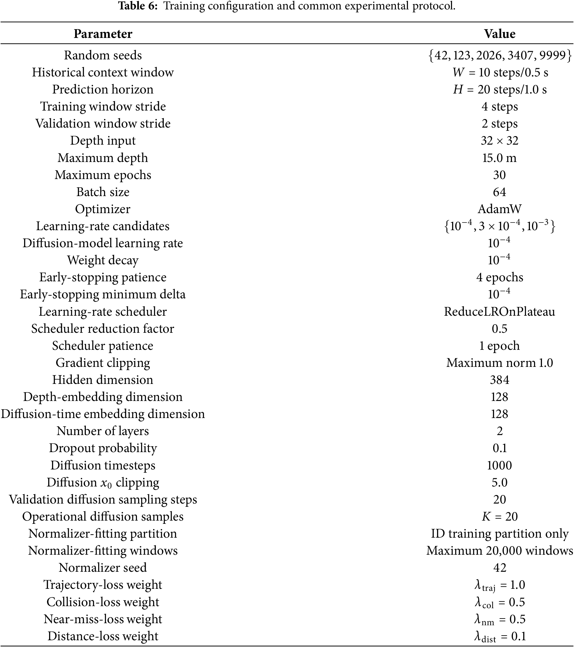
The loss weights used in the reviewer-aligned training pipeline are

λtraj=1.0,λcol=0.5,λnm=0.5,λmd=0.1.(18)

Positive-class weights are estimated from the ID training partition for collision and near-miss prediction to mitigate class imbalance. No validation or test samples are used when estimating these training statistics.

3.5.5 DDIM-Based Inference and Control-Oriented Interpretation

At inference time, the model starts from Gaussian noise and performs a DDIM-style reverse-diffusion process to generate a future relative trajectory. The final denoised trajectory is passed to the three supervised heads to obtain horizon-wise collision probabilities, near-miss probabilities, and minimum-distance estimates. Because the reverse process starts from a random Gaussian sample, multiple trajectory rollouts can be generated for the same historical context. Let M denote the number of sampled rollouts. A downstream planner or safety supervisor may aggregate these sampled trajectories to estimate probabilistic collision risk:

ptcol=1M∑m=1MI[min1≤h≤Hd^t+h(m)≤rUAV],(19)

where d^t+h(m) denotes the predicted minimum obstacle distance at the h-th step of the m-th sampled rollout. For downstream control integration, the predicted risk can additionally support an adaptive minimum-safe-distance threshold:

dtsafe=d0+ασt+β[vtrel]++γptcol,(20)

where d0 is a baseline safety margin, σt denotes rollout dispersion, vtrel denotes the relative closing speed, [⋅]+=max(0,⋅), and α, β, and γ are non-negative coefficients. The sampled-rollout aggregation rule and adaptive safety-distance formulation define the interface between the predictive world model and the downstream safety-aware decision module. Open-loop experiments evaluate forecasting, uncertainty, and calibration, while the revised closed-loop benchmark evaluates learned-model rollouts separately. Oracle simulator rollouts, where retained, are treated only as a reference upper bound.

4  Experimental Setup

4.1 Simulation Workflow and Reproducibility Scope

The experimental workflow follows the Gazebo-assisted hybrid simulation pipeline described in the methodology. Gazebo is used for base-environment construction and representative scenario verification, whereas the retained Python/NumPy automation layer performs procedural obstacle randomization, disturbance injection, geometry-based sensing synthesis, synchronized logging, and future-risk annotation. The simulated workspace is 15×15×8 m3, the simulation timestep is 0.05 s, and the sampling frequency is 20 Hz. Each episode contains 200 timesteps and therefore represents 10 s of simulated flight. The complete ID dataset contains 1000 episodes and 200,000 temporally synchronized frames. The retained dataset is geometry-driven rather than photorealistic. It includes RGB observations, depth maps, UAV states, control actions, obstacle states, point clouds, occupancy grids, and future-risk labels. The trained models use the historical state-action context, current safety context, and current depth map according to the matched-input protocol; the remaining modalities are retained for dataset completeness and future architectural extensions.

4.2 Episode-Level Dataset Partitioning

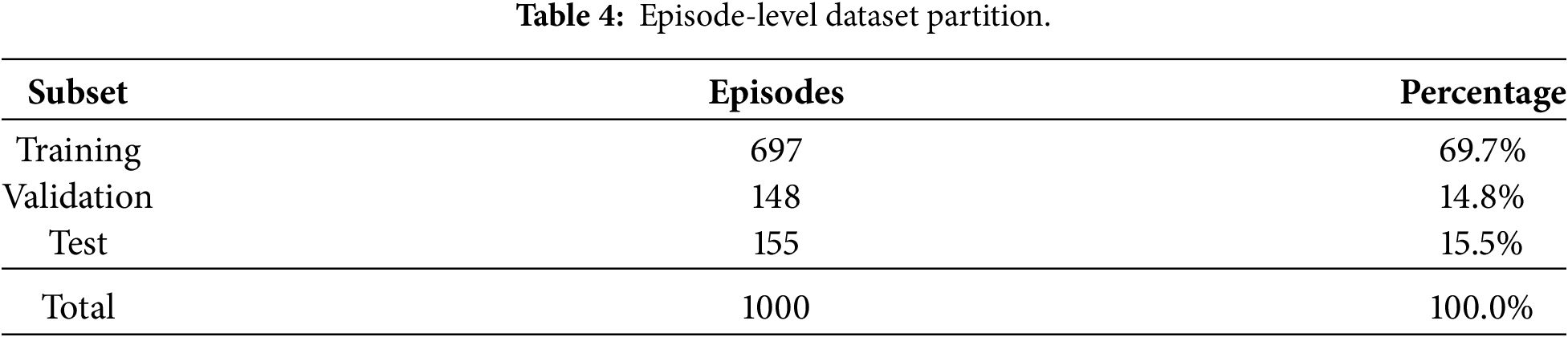
The dataset is partitioned at the episode level rather than at the frame or sliding-window level. This protocol prevents temporally adjacent observations from the same UAV trajectory from appearing in different subsets, thereby reducing temporal leakage. A fixed and reproducible split is used for all model families, ablation variants, random seeds, and evaluation procedures. The revised partition contains 697 training episodes, 148 validation episodes, and 155 test episodes. These subsets are mutually exclusive and jointly contain all 1000 episode identifiers. Table 4 reports the exact partition sizes and percentages; the 69.7/14.8/15.5 split is shared unchanged by the proposed model, all recurrent baselines, and every ablation experiment.

Each learning sample uses a historical context of W=10 timesteps and predicts a future horizon of H=20 timesteps. Sliding windows are constructed independently within each episode and retain the corresponding episode_id. Different strides are used according to the role of each subset: a stride of four for training, two for validation, and one for threshold selection and final testing. Importantly, overlapping sliding windows are used as optimization samples but are not treated as statistically independent observations during uncertainty estimation. Window-level predictions are first associated with their source episodes, after which uncertainty is quantified using the episode as the resampling unit. This avoids artificially narrow confidence intervals caused by treating strongly overlapping temporal windows as independent samples. All preprocessing statistics are estimated exclusively from the ID training partition. Normalization statistics are fitted using at most 20,000 training windows selected with a fixed normalizer seed of 42. The preprocessing manifest records the immutable training-partition signature and the corresponding normalization artifacts. Validation and test episodes are excluded from normalization fitting and model training.

4.3 Implementation Environment

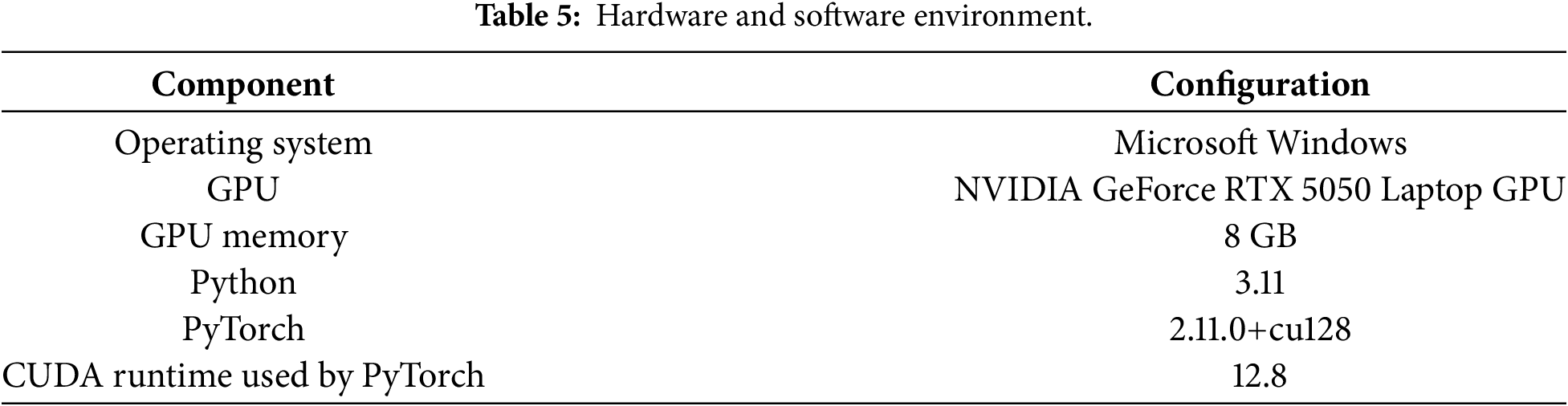
The experiments are executed under Microsoft Windows using an NVIDIA GeForce RTX 5050 Laptop GPU with 8 GB of video memory. The reviewer-aligned environment uses Python 3.11 and PyTorch 2.11.0 with CUDA 12.8 support. The implementation platform is summarized in Table 5. Reporting the software stack and GPU configuration improves reproducibility because diffusion inference time and numerical behavior can depend on the CUDA/PyTorch environment.

4.4 Training Configuration and Common Experimental Protocol

All model families are trained under a matched experimental protocol designed to support statistically fair comparison. Five independent training seeds, {42,123,2026,3407,9999}, are used for every experiment. All models use the same immutable episode-level split, historical context length, prediction horizon, preprocessing artifacts, validation partition, and evaluation partition. Architecture-specific learning rates are selected from the common candidate set {10−4,3×10−4,10−3}. The resulting learning rates are 3×10−4 for the GRU, LSTM, hybrid GRU-LSTM, deterministic, and risk-only families, and 10−4 for the diffusion family and its diffusion-based ablations. Final training uses a common maximum budget of 30 epochs. Early stopping is applied with a patience of four epochs and a minimum improvement threshold of 10−4. AdamW optimization is used with weight decay 10−4 and gradient clipping at a maximum norm of 1.0. A ReduceLROnPlateau scheduler reduces the learning rate by a factor of 0.5 after one validation epoch without sufficient improvement. The maximum epoch count is interpreted as a common computational cap rather than as evidence of convergence. Checkpoints are selected using validation performance under the same rule for every architecture, and runs reaching the cap are retained in the convergence audit so that the training budget is reported transparently. The complete shared optimization settings are consolidated in Table 6. The common data split, preprocessing protocol, history/horizon, learning-rate candidate set, and early-stopping rule are held fixed across model families so that architectural comparisons are not confounded by different training procedures.

4.5 Full-Test Predictive Evaluation and Statistical Protocol

All final predictive results are computed on the complete held-out ID test partition. No ordered 1024-window subset is used in the revised evaluation. The test loader traverses all valid test windows, while each prediction retains the corresponding episode identifier to preserve the hierarchical temporal structure of the data.

Trajectory forecasting is evaluated using average displacement error (ADE) and final displacement error (FDE):

ADE=1NH∑i=1N∑h=1H‖p^i,h−pi,h‖2,(21)

FDE=1N∑i=1N‖p^i,H−pi,H‖2.(22)

Because diffusion prediction is intrinsically stochastic, the proposed model is additionally evaluated using K={5,10,20} future samples for each conditioning input. We report meanADE@K and meanFDE@K to characterize average sampled quality, minADE@K and minFDE@K to measure best-of-K future coverage, and trajectory and endpoint diversity to quantify the dispersion of plausible sampled futures.

Collision and near-miss probabilities are evaluated using precision, recall, F1-score, Brier score, and expected calibration error (ECE). ECE is computed using 15 probability bins. Classification thresholds are selected exclusively on the ID validation partition using a fixed threshold-selection procedure and are frozen before evaluation on the ID test and OOD partitions. Reliability diagrams are used to visualize the relationship between predicted probability and empirical event frequency.

To account for the statistical dependence introduced by overlapping sliding windows, uncertainty is evaluated at the episode level. Predictions from windows belonging to the same episode are grouped before statistical resampling. Episode-level bootstrap with 5000 replicates and a fixed bootstrap seed is used to estimate 95% confidence intervals. In addition, each model is trained using five independent random seeds, and seed-level variability is reported using the mean and sample standard deviation across the five runs.

4.6 Matched Baselines and Ablation Models

The revised comparison includes recurrent, deterministic, generative, and risk-only architectures trained under the same episode-level data partitions and common experimental protocol. Table 7 summarizes the evaluated model families and their corresponding roles in the comparative analysis.

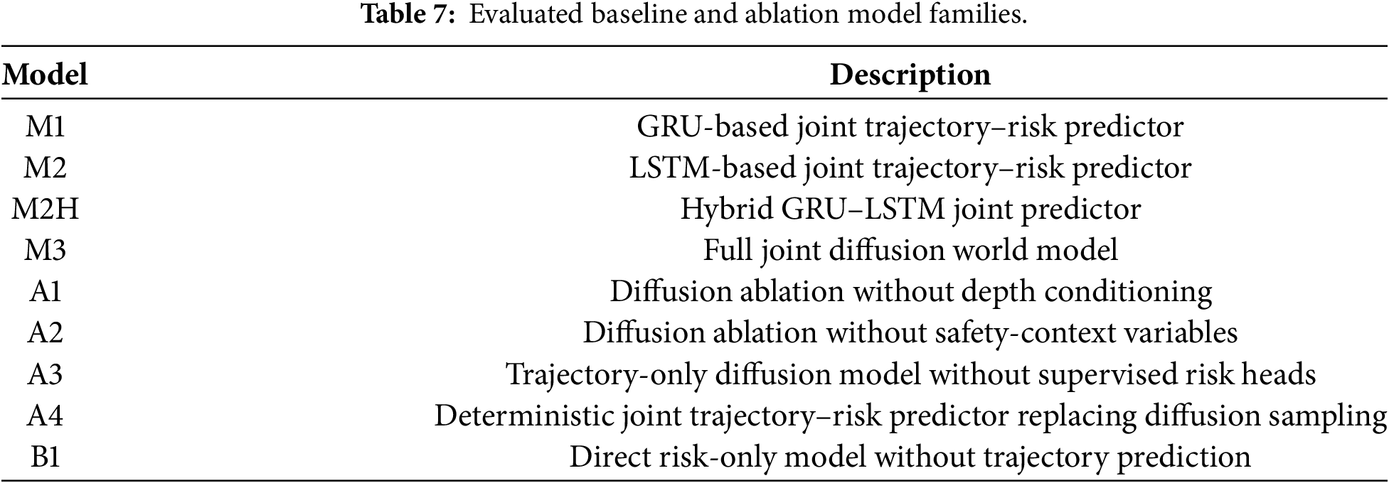
Except when an input is intentionally removed as part of an ablation, matched models receive the same state, action, depth, and safety-context information, together with the same historical context W=10 and prediction horizon H=20. All model families use the same preprocessing artifacts, episode-level split, learning-rate candidate set, early-stopping policy, and five training seeds. This design enables differences in performance to be attributed more directly to architectural or input changes rather than to inconsistent data or optimization procedures.

4.7 Offline OOD Generalization Protocol

Generalization is evaluated without retraining or threshold adjustment on the independent 300-episode OOD test suite introduced in Fig. 1 and Table 3. Each OOD profile contains 100 episodes. OOD Sparse/Fast increases the number and speed of dynamic obstacles, OOD Dense/Small substantially increases obstacle density while reducing obstacle size, and OOD Large introduces obstacle sizes outside the ID training range. For every trained seed, the corresponding checkpoint is evaluated on the complete OOD partition with the same preprocessing artifacts and the collision and near-miss thresholds selected on ID validation. No OOD labels are used for model selection, calibration, or threshold tuning.

The same trajectory, risk, calibration, and multimodal metrics used on ID are recomputed on each OOD profile. Consequently, OOD analysis does not reduce generalization to a single trajectory-error score: ADE/FDE and best-of-K coverage are considered together with collision F1, near-miss F1, Brier score, and ECE. This is important because a distribution shift may affect geometric forecasting and probabilistic safety estimation differently.

4.8 Learned-Model Closed-Loop Evaluation Protocol

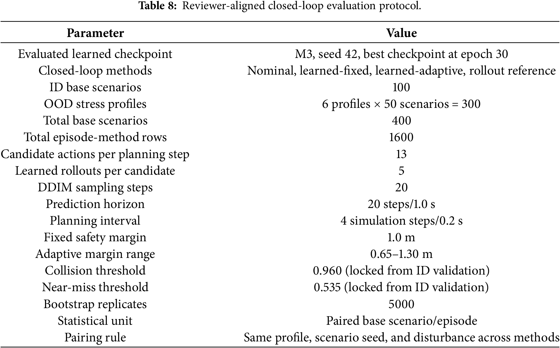
A separate closed-loop stress test evaluates whether the learned diffusion model can be integrated end-to-end into online candidate-action selection. The closed-loop benchmark is inference-only and uses the M3 checkpoint trained with seed 42; therefore, this experiment is intended to test predictive-safety integration rather than to establish a closed-loop ranking between M3 and the recurrent baselines. The locked collision and near-miss thresholds are 0.960 and 0.535, respectively, both selected from ID validation before closed-loop evaluation. No threshold is re-optimized on ID test or OOD scenarios.

Four decision strategies are compared: (i) the nominal controller without predictive intervention, (ii) learned-fixed, which evaluates candidate actions with the learned model and a fixed 1.0 m safety margin, (iii) learned-adaptive, which uses learned trajectory dispersion, closing speed, and collision risk to adapt the safety margin between 0.65 and 1.30 m, and (iv) a short-horizon simulator rollout reference. The rollout reference is included as a computationally expensive simulator-based comparator and is not treated as a mathematical upper bound.

At each planning update, 13 candidate actions are considered. The learned planners use five stochastic rollouts per candidate with 20 DDIM sampling steps and a prediction horizon of 20 simulator steps. Planning is performed every four simulation steps. The action-selection objective combines collision, near-miss, goal-progress, clearance, and control-deviation costs. The adaptive planner uses a base safety margin of 0.65 m, dispersion weight 0.8, closing-speed weight 0.25, and collision-risk weight 0.6. The corresponding fixed and adaptive settings are summarized in Table 8.

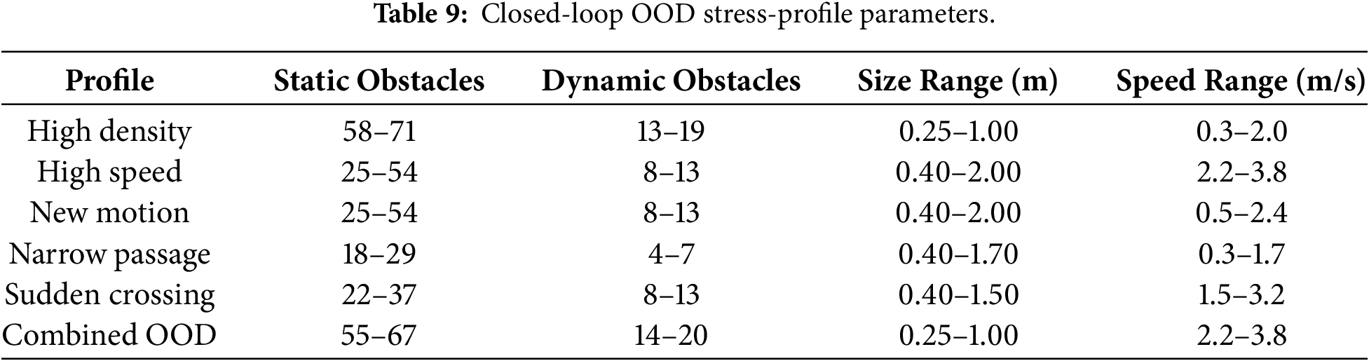
The closed-loop OOD suite is deliberately broader than the three-profile offline OOD suite. It contains high-density, high-speed, new-motion, narrow-passage, sudden-crossing, and combined-OOD stress profiles. Table 9 reports the generation ranges. The narrow-passage profile uses a 1.15 m passage gap, the sudden-crossing profile activates crossing motion at 1.5 s, and the combined-OOD profile combines high density, high speed, new motion, narrow passage, and sudden crossing.

Each scenario is assigned one disturbance condition from a fixed schedule comprising nominal dynamics, observation noise, wind gust, action delay, action noise, and obstacle-position perturbation. The observation perturbation uses position and velocity standard deviations of 0.08 m and 0.12 m/s; wind-gust force has a standard deviation of 1.2 N; the action delay is two simulator steps; and obstacle-position jitter has a standard deviation of 0.12 m. All four methods receive the same scenario seed and disturbance assignment, enabling paired comparisons.

Closed-loop outcomes include success rate, collision-episode rate, near-miss-episode rate, minimum clearance, time-to-goal for successful episodes, path length, computation time, recovery, and failure mode. Uncertainty is quantified using 5000 paired base-scenario/episode bootstrap replicates. A paired difference is interpreted as conclusive only when its 95% confidence interval excludes zero.

5  Results and Discussion

5.1 Full-Test Performance Across Independent Training Seeds

Table 10 summarizes performance on the complete ID test partition. Each value is reported as the mean and sample standard deviation across five independently trained seeds. The recurrent models achieve substantially lower conventional single-trajectory ADE and FDE than the stochastic diffusion model. M1 obtains an ADE of 0.4083±0.0333 m, M2 obtains 0.4114±0.0246 m, and M2H obtains 0.4127±0.0489 m. The deterministic A4 predictor obtains 0.4524±0.0510 m. In comparison, the full diffusion model M3 obtains a single-sample ADE of 0.8843±0.0339 m and FDE of 1.6965±0.0442 m.

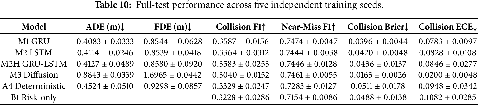
These results show that the principal advantage of the diffusion model becomes clearer when multimodal future coverage and probabilistic safety estimation are considered. In particular, M3 achieves a collision Brier score of 0.0163±0.0026 and collision ECE of 0.0200±0.0048, substantially lower than the corresponding values of the direct risk-only and deterministic baselines. The recurrent predictors therefore remain strong deterministic trajectory forecasters, whereas the diffusion formulation provides a complementary representation of future uncertainty and calibrated collision risk.

Fig. 3 visualizes the five seed-level test values underlying the aggregate statistics in Table 10. The boxplots make the between-seed spread explicit and help distinguish stable performance trends from results that may be sensitive to initialization or stochastic optimization.

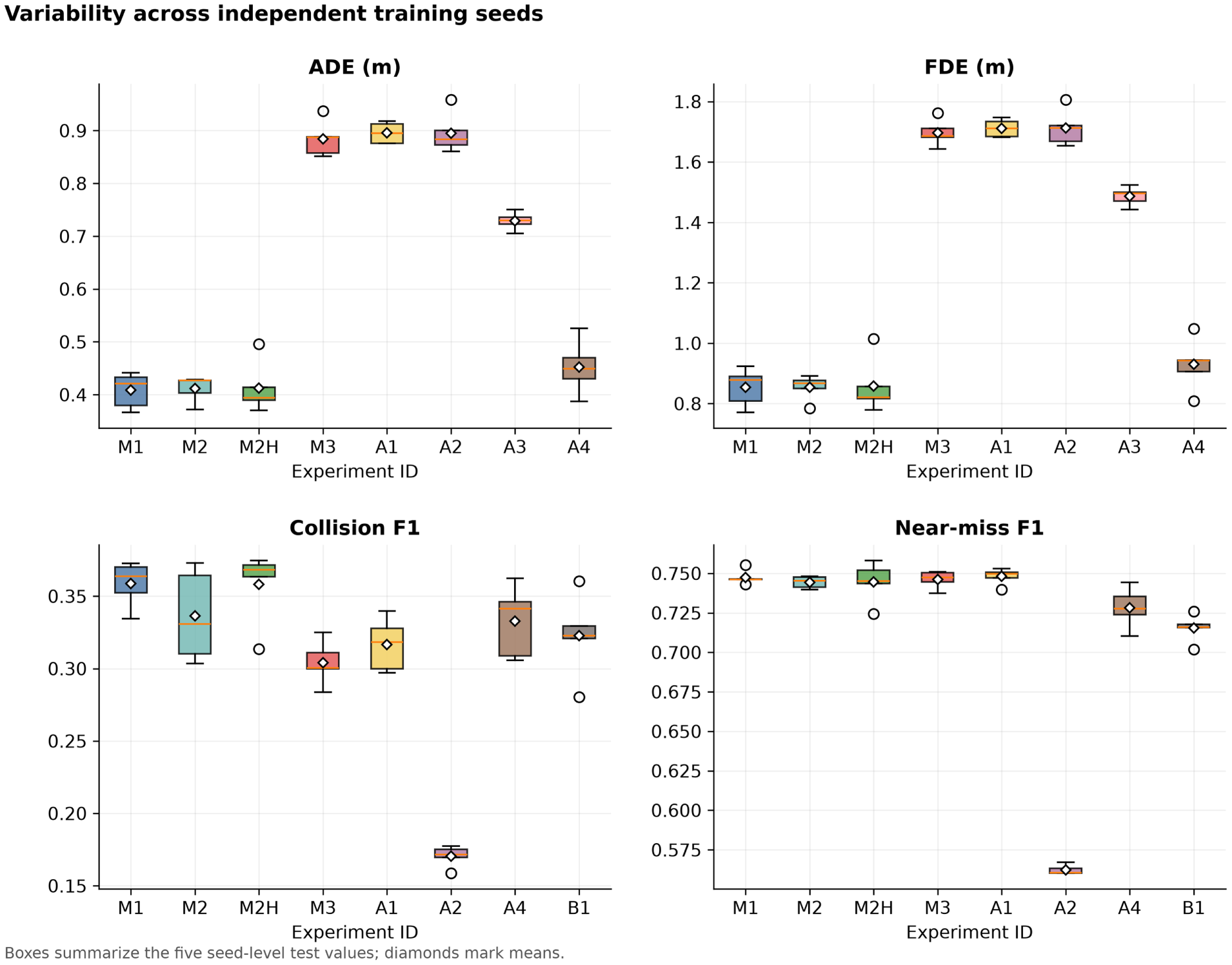
Figure 3: Variability across five independent training seeds for ADE, FDE, collision F1, and near-miss F1. Boxes summarize seed-level test values and diamonds denote their means.

5.2 Ablation Analysis

The ablation experiments quantify the contribution of depth conditioning, safety-context variables, supervised risk heads, and diffusion-based stochastic prediction. Removing depth information (A1) produces only a modest degradation relative to M3 under the ID test distribution, suggesting that the numerical state-action and safety-context representation already contains substantial predictive information in the current synthetic environment. Table 11 summarizes the component-wise ablation results across the same five seeds. Reading the table together with the preceding discussion shows that removing safety context produces the clearest deterioration in risk prediction, whereas removing depth has a smaller effect under the current ID distribution.

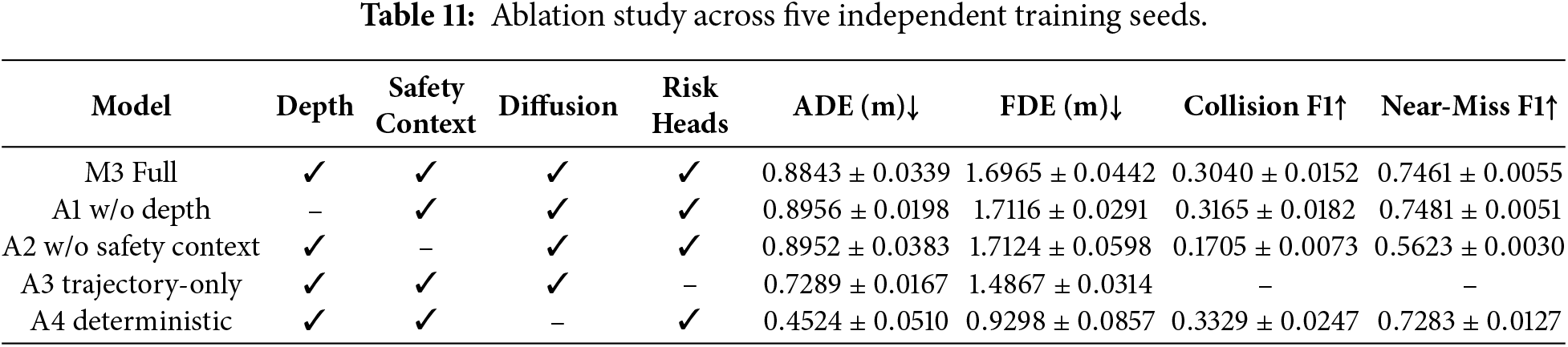
In contrast, removing the safety context (A2) causes a pronounced degradation in risk prediction. Collision F1 decreases from 0.3040±0.0152 for M3 to 0.1705±0.0073, while near-miss F1 decreases from 0.7461±0.0055 to 0.5623±0.0030. Near-miss Brier score also increases from approximately 0.130 to 0.216. These results indicate that the safety-context variables play an important role in distinguishing geometrically similar motion states with different immediate risk levels. The trajectory-only diffusion ablation A3 produces substantially lower displacement error than the joint M3 model, with ADE 0.7289±0.0167 and FDE 1.4867±0.0314. This trade-off suggests that jointly optimizing trajectory generation and supervised risk estimation modifies the learned representation toward safety-relevant prediction rather than minimum displacement error alone.

5.3 Direct Risk Prediction vs. Joint Trajectory-Risk Modeling

The B1 risk-only baseline directly predicts collision and near-miss probabilities without producing a future trajectory. This experiment addresses whether collision risk can be estimated without explicit trajectory forecasting. B1 achieves a collision F1-score of 0.3228±0.0286, which is slightly higher than the 0.3040±0.0152 obtained by M3. However, the joint diffusion model produces substantially better calibrated collision probabilities: its Brier score decreases from 0.0488±0.0138 for B1 to 0.0163±0.0026, while collision ECE decreases from 0.1082±0.0285 to 0.0200±0.0048. Therefore, direct collision prediction is feasible and can remain competitive in thresholded classification metrics. Nevertheless, the joint trajectory-risk formulation provides additional information about plausible future motion and yields markedly better calibrated collision probabilities, which are advantageous when risk estimates are consumed by downstream decision-making rather than interpreted only as binary labels.

5.4 Multimodal Future Prediction

The principal motivation for using a diffusion model is its ability to represent multiple plausible futures rather than a single deterministic trajectory. To evaluate this property, the full M3 model is sampled using K={5,10,20} futures for the same conditioning input. Table 12 reports both average-sample and best-of-K errors. This distinction is important because meanADE/meanFDE describe the typical sampled trajectory, whereas minADE/minFDE measure whether at least one sampled future captures a plausible ground-truth mode.

The average sampled displacement remains nearly constant as K increases, indicating that simply drawing more samples does not improve the accuracy of each individual trajectory. In contrast, the best-of-K errors decrease consistently. minADE decreases from approximately 0.536 m at K=5 to 0.396 m at K=20, while minFDE decreases from approximately 0.967 to 0.644 m. This behavior demonstrates that additional diffusion samples increase coverage of plausible future modes rather than collapsing toward the same deterministic prediction.

At K=20, the mean trajectory-diversity metric is 0.9409±0.0621, while endpoint diversity is 1.7247±0.0840. The non-zero diversity together with the systematic decrease in best-of-K error provides quantitative evidence that the diffusion branch generates distinct plausible futures.

5.5 Probabilistic Calibration

Probability calibration is important because a downstream safety supervisor may use risk probabilities directly rather than only their thresholded binary decisions. For this reason, collision and near-miss predictions are evaluated using Brier score, expected calibration error, and reliability diagrams.

For the full diffusion model, the collision Brier score is 0.0163 ± 0.0026 and collision ECE is 0.0200 ± 0.0048. The corresponding near-miss Brier score is 0.1296 ± 0.0017, with an ECE of 0.0767 ± 0.0050. Classification thresholds are selected exclusively using the ID validation partition and are frozen before evaluation of the ID test and OOD datasets. Fig. 4 visualizes calibration for collision risk, while Fig. 5 provides the corresponding near-miss analysis. In both diagrams, the dashed diagonal represents perfect calibration; deviations from this line indicate probability ranges in which the predicted confidence differs from the empirical event frequency.

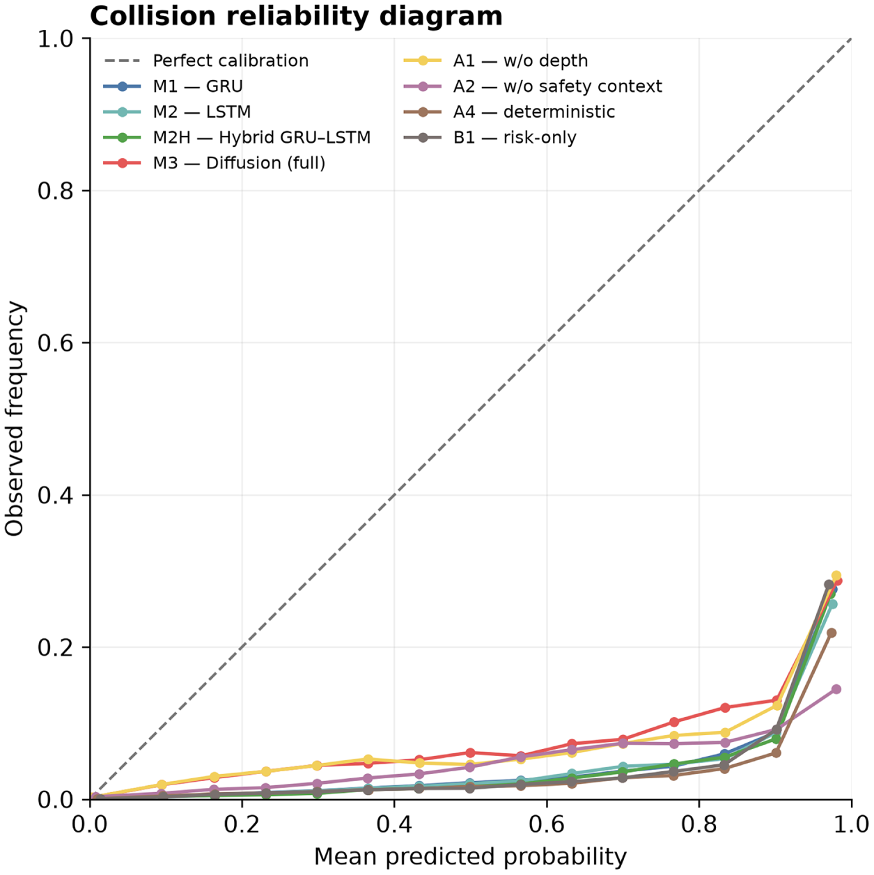
Figure 4: Reliability diagram for collision-risk prediction. The dashed diagonal denotes perfect calibration.

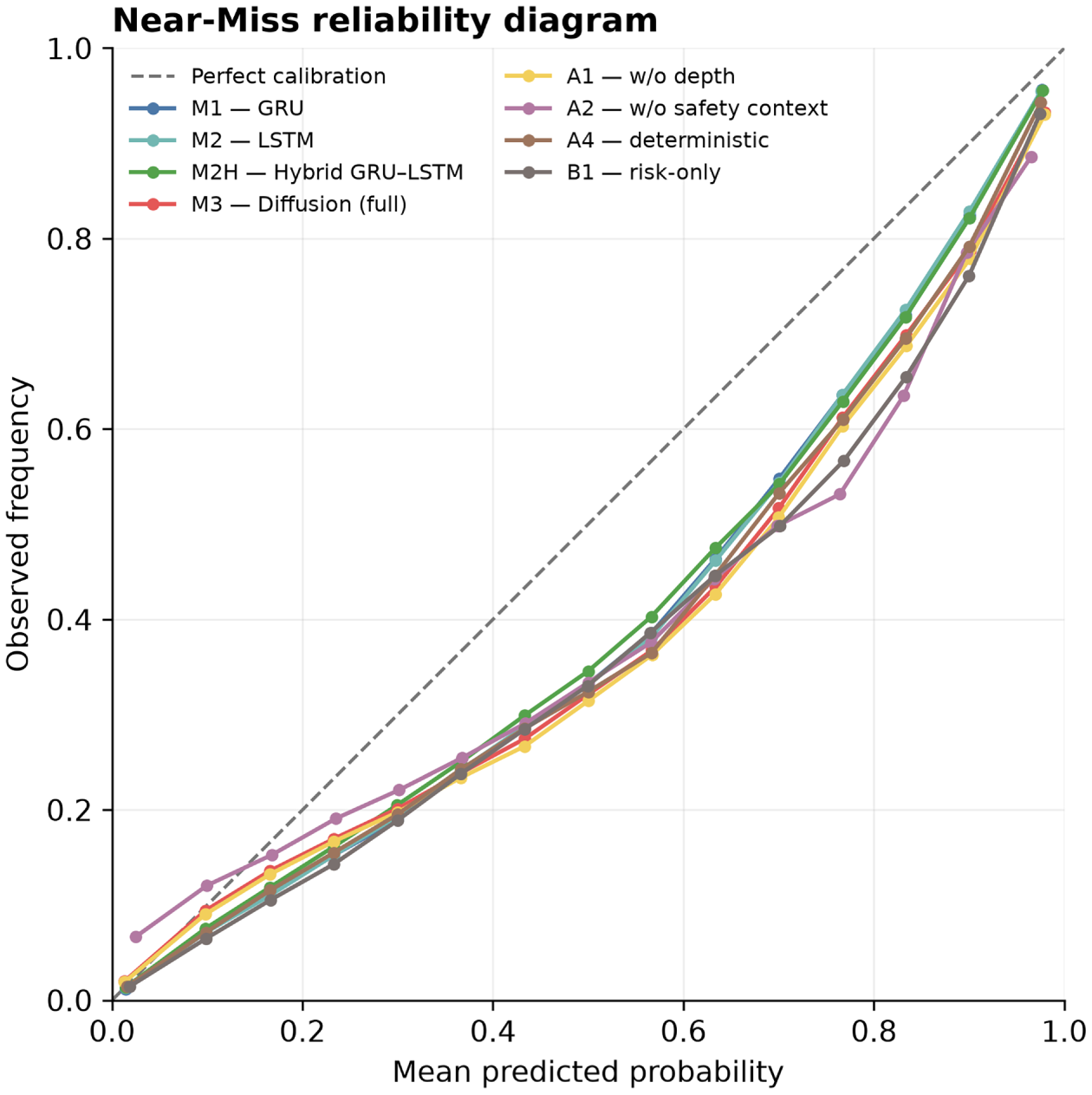
Figure 5: Reliability diagram for near-miss probability prediction. The dashed diagonal denotes perfect calibration.

Taken together, Figs. 4 and 5 show that calibration quality is task dependent. The collision task is summarized by a particularly low ECE for M3, whereas near-miss prediction remains more difficult to calibrate because it covers a broader transition region between clearly safe and collision states. These diagrams therefore complement thresholded F1 scores by evaluating whether the reported probabilities themselves are suitable for downstream risk-aware decision making.

5.6 Out-of-Distribution Generalization

To evaluate robustness to previously unseen obstacle distributions, the trained models are evaluated without additional optimization on three OOD profiles: OOD Sparse/Fast, OOD Dense/Small, and OOD Large. These profiles respectively modify obstacle velocity and population, increase obstacle density while reducing obstacle size, and introduce obstacle sizes beyond the ID training range.

Table 13 compares the full M3 diffusion model on the ID test partition and the three offline OOD profiles. All values are reported as mean±SD across the same five independent training seeds. The results show that OOD behavior is configuration dependent rather than uniformly degraded.

OOD Sparse/Fast produces only a modest increase in geometric trajectory error: relative to ID, ADE rises from 0.8843 to 0.9120 m and FDE from 1.6965 to 1.7607 m. In contrast, calibration deteriorates much more strongly. Collision Brier score increases from 0.0163 to 0.0538 and collision ECE from 0.0200 to 0.0543, while near-miss F1 decreases from 0.7461 to 0.6402. This profile therefore reveals a failure mode in which trajectory geometry remains comparatively stable while probabilistic safety estimates become less reliable under previously unseen obstacle speeds.

OOD Dense/Small exhibits a different failure pattern. ADE, FDE, minADE@20, and minFDE@20 are numerically lower than on ID, yet collision F1 decreases from 0.3040 ± 0.0152 to 0.1482 ± 0.0133, a reduction of approximately 51.3%. Thus, improved displacement metrics do not imply improved collision-risk recognition under distribution shift. The same profile is difficult across model families rather than uniquely for diffusion: collision F1 decreases to approximately 0.1623 for M1, 0.1700 for M2, 0.1744 for M2H, 0.1429 for A4, and 0.1366 for B1.

Conversely, OOD Large is comparatively easier for several safety metrics. M3 collision F1 increases to 0.4237±0.0178, while collision Brier and ECE decrease to 0.0105±0.0025 and 0.0179±0.0044, respectively. Accordingly, the OOD experiments do not support a claim that all unseen configurations necessarily degrade performance. Instead, they show that generalization depends on the specific type of distribution shift and that geometric forecasting and calibrated risk estimation can fail independently.

These results directly answer the reviewer question concerning unseen obstacle configurations: the model can fail or become poorly calibrated under specific OOD conditions, particularly dense-small and sparse-fast scenarios. Explicit OOD evaluation is therefore necessary before using trajectory accuracy alone as evidence of safety robustness.

5.7 Learned-Model Closed-Loop Evaluation

The revised closed-loop experiment evaluates whether the learned predictive model can support action selection without relying on oracle simulator future dynamics as the primary rollout mechanism. Candidate actions are evaluated using future trajectories and risk estimates generated by the learned model. Multiple disturbance rollouts are used to characterize candidate-level risk, and the same scenario seeds are shared across methods to enable paired comparison.

The benchmark reports success rate, collision episode rate, near-miss rate, minimum obstacle clearance, time-to-goal, path length, and computation time together with episode-level statistical uncertainty. Oracle simulator rollouts are retained only as an upper-bound reference.

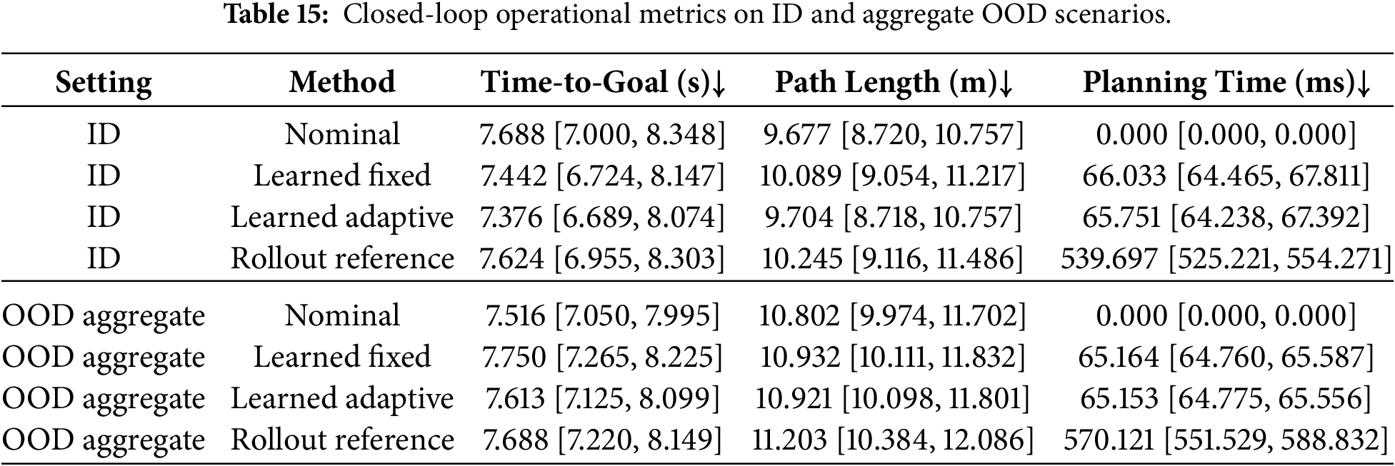
The final closed-loop benchmark contains 400 paired base scenarios and four methods, yielding 1600 episode-method rows. The ID portion contains 100 scenarios, while the closed-loop OOD stress suite contains 300 scenarios across six profiles. Tables 14 and 15 summarize ID and aggregate-OOD performance. The brackets report 95% base-scenario/episode bootstrap confidence intervals.

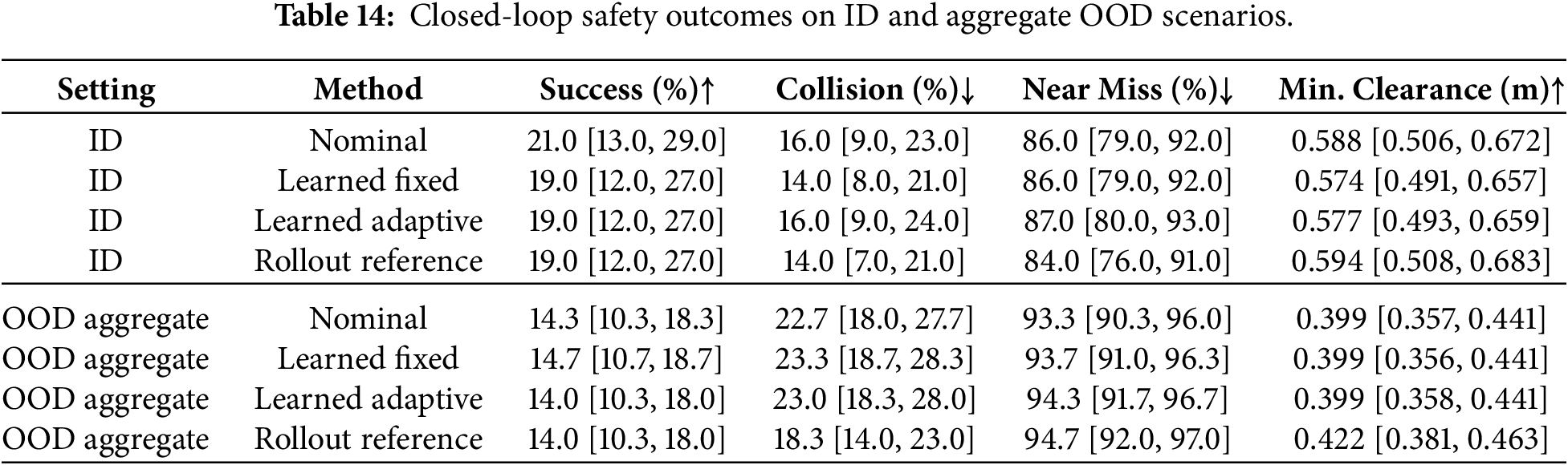
On ID, learned-fixed produces a modest numerical reduction in collision rate from 16% to 14%. However, its paired collision-rate difference relative to nominal is −2 percentage points with a 95% CI of [−6,+2], which includes zero. The success rate also changes from 21% to 19%. Learned-adaptive yields the same 16% collision rate as nominal. Consequently, the ID experiment does not support a statistically conclusive claim that the learned planner reduces collision probability, although learned-fixed shows a small numerical improvement.

The aggregate OOD results are more challenging. Nominal collision rate is 22.7%, compared with 23.3% for learned-fixed and 23.0% for learned-adaptive. Success remains low for all methods, between approximately 14.0% and 14.7%. These results show that the learned safety benefit does not transfer uniformly to unseen closed-loop scenarios. The rollout reference reduces aggregate OOD collision rate to 18.3% and increases mean minimum clearance to 0.422 m, but at substantially greater computation cost.

The strongest practical advantage of learned-model planning is computation time. Across ID and aggregate OOD, learned-fixed and learned-adaptive require approximately 65–66 ms per planning decision, whereas the short-horizon rollout reference requires approximately 540 ms on ID and 570 ms on aggregate OOD. Thus, the learned model provides an order-of-magnitude reduction in planning latency relative to simulator rollout, although its safety improvement is not uniform.

Fig. 6 visualizes collision-episode rates across ID and the closed-loop OOD stress profiles. The variation across profiles makes clear that collision behavior is scenario dependent rather than described adequately by a single aggregate percentage.

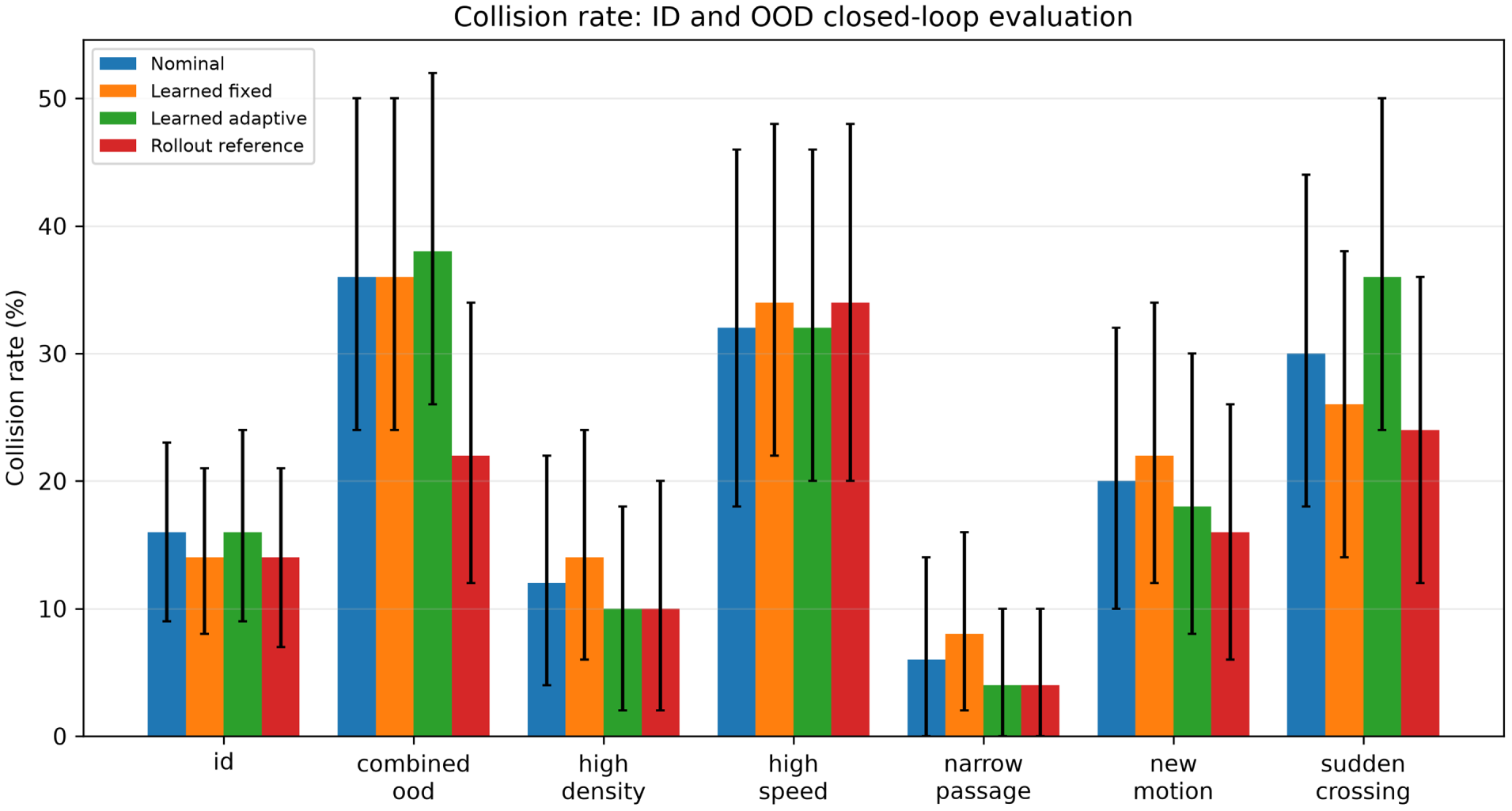
Figure 6: Closed-loop collision-episode rate across ID and OOD stress profiles for the nominal, learned-fixed, learned-adaptive, and short-horizon rollout-reference methods.

Fig. 7 shows the corresponding planning-time comparison. The learned approaches maintain planning times near 65 ms across profiles, whereas the simulator rollout reference requires several hundred milliseconds and becomes particularly expensive in difficult OOD scenarios.

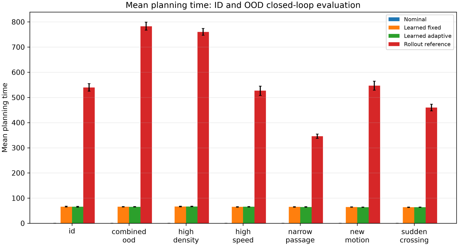
Figure 7: Mean closed-loop planning time across ID and OOD stress profiles. The learned planners are substantially faster than the short-horizon simulator rollout reference.

The most difficult profile is Combined OOD, which simultaneously introduces high obstacle density, high speed, unseen motion behavior, narrow-passage geometry, and sudden crossing. Table 16 shows that learned-fixed does not reduce collision rate relative to nominal (36% vs. 36%), while learned-adaptive increases it numerically to 38%. The rollout reference reduces collision rate to 22% and increases minimum clearance from 0.155 to 0.230 m, but its planning time rises to approximately 782 ms.

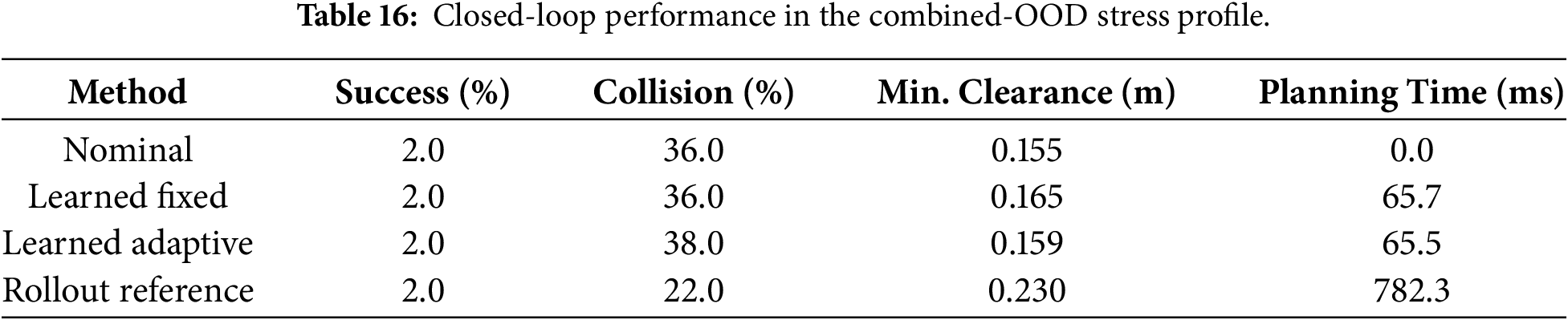
The paired minimum-clearance improvement of the rollout reference over nominal in Combined OOD is +0.0749 m with a 95% CI of [+0.0206,+0.1353] m, which excludes zero. In contrast, the learned-fixed collision difference is 0 percentage points with a CI of [−8,+8], and the learned-adaptive difference is +2 points with a CI of [−6,+12]. Therefore, the simulator reference exhibits a measurable clearance advantage in this hardest configuration, but this benefit comes with substantially greater latency.

Failure analysis further shows that low success is not explained by collision alone. In Combined OOD, goal_not_reached accounts for 56% of nominal episodes, 58% of learned-fixed episodes, 58% of learned-adaptive episodes, and 66% of rollout-reference episodes. The corresponding success rate is only 2% for every method. Consequently, the closed-loop benchmark should be interpreted as a stress test of predictive-safety integration rather than evidence that the current system solves end-to-end autonomous navigation.

Overall, the closed-loop experiment satisfies the requested protocol requirements-paired scenarios, increased episode count, multiple stochastic rollouts, disturbances, learned-model action selection, operational metrics, failure analysis, and episode-level confidence intervals-but the efficacy result is deliberately more limited. The learned diffusion planner is computationally much cheaper than simulator rollout and can be executed end-to-end, yet its collision benefit is scenario dependent and is not statistically uniform across ID and OOD conditions.

5.8 Limitations and Future Work

Several limitations remain despite the expanded reviewer-aligned evaluation. First, all training data are generated in simulation. Although the data-generation process randomizes obstacle geometry, dynamic motion, sensing noise, controller behavior, and disturbances, the synthetic environment does not reproduce the full photometric, aerodynamic, sensing, and actuation complexity of a physical UAV. Real deployment may introduce depth artifacts, localization drift, actuator latency, aerodynamic-model mismatch, communication delay, wind-field structure, and perception failures that are absent or simplified in the current simulator. Accordingly, the present results should be interpreted as simulation-based evidence rather than real-world flight validation.

Second, the OOD experiments reveal that generalization failure is metric and scenario dependent. The offline Sparse/Fast profile causes relatively small trajectory-error changes but markedly worse collision and near-miss calibration, while Dense/Small reduces collision F1 despite improved displacement metrics. Conversely, the Large-obstacle profile improves several risk metrics. The closed-loop stress suite extends this analysis to high-density, high-speed, new-motion, narrow-passage, sudden-crossing, and combined shifts, but it still cannot represent the open-ended range of real-world distribution changes. Future work should therefore incorporate explicit OOD detection, uncertainty-triggered fallback behavior, online calibration monitoring, and adaptation using previously unseen environmental conditions.

Third, deterministic recurrent models remain stronger in conventional single-trajectory ADE and FDE. The empirical benefit of diffusion lies in multimodal future coverage and calibrated probabilistic collision risk rather than uniformly superior point forecasting. Moreover, the trajectory-only diffusion ablation improves geometric trajectory accuracy, revealing a measurable multi-task trade-off between pure displacement optimization and joint safety supervision. Future architectures should investigate decoupled or dynamically weighted objectives that preserve risk calibration while reducing single-trajectory error.

Fourth, the closed-loop results do not demonstrate a uniform safety improvement over the nominal controller. Learned-fixed reduces ID collision rate numerically from 16% to 14%, but the paired 95% confidence interval of the difference includes zero. Aggregate OOD collision rates for learned-fixed and learned-adaptive are comparable to or slightly higher than nominal, and Combined OOD remains particularly challenging. In addition, success rates are low because many episodes terminate without reaching the goal even when no collision occurs. Future work should therefore jointly optimize safety and task progress rather than treating collision avoidance as the only control objective.

Fifth, the current learned closed-loop benchmark uses the M3 checkpoint from seed 42 rather than repeating the full closed-loop evaluation for every architecture and all five training seeds. This design satisfies the reviewer request for an end-to-end learned-model test but does not establish that diffusion is superior to GRU, LSTM, or deterministic models in closed-loop control. A future paired benchmark should compare multiple learned model families under the identical candidate-action and disturbance protocol.

Finally, computation remains an important deployment constraint. Learned diffusion planning requires approximately 65 ms per planning update in the present implementation, which is substantially faster than the 0.35–0.78 s short-horizon simulator rollout reference but remains above the 50 ms base simulation timestep. Practical deployment will therefore require accelerated diffusion sampling, reduced-step solvers, model distillation, candidate pruning, asynchronous planning, or lower-frequency supervisory integration. A staged sim-to-real program combining stronger domain randomization, hardware-in-the-loop testing, UAV system identification, physical sensor-noise characterization, and fine-tuning on real flight logs is planned before any real-world safety claims are made.

6  Conclusion

This study presents a hybrid diffusion world model for short-horizon UAV trajectory forecasting and probabilistic collision-risk estimation in dense three-dimensional environments. The revised framework combines historical UAV state-action information, depth observations, and safety-context variables to generate multiple plausible future trajectories while jointly estimating collision, near-miss, and obstacle-clearance information. The experimental protocol was redesigned to address the principal methodological concerns raised during review. The 1000-episode ID dataset is split exclusively at the episode level into 697 training, 148 validation, and 155 test episodes. All baseline and ablation families use the same immutable partitions, preprocessing artifacts, historical context, prediction horizon, learning-rate candidate set, and early-stopping rule. Nine configurations are trained with five independent random seeds, and the complete ID test partition is evaluated rather than an ordered subset of windows. Statistical uncertainty is handled at the episode level using 5000 bootstrap replicates, while collision and near-miss thresholds are selected only on ID validation and then frozen for test and OOD evaluation.

The results do not support the claim that diffusion is a better single deterministic trajectory predictor. GRU, LSTM, and hybrid recurrent baselines achieve substantially lower conventional ADE and FDE. Instead, the main advantage of M3 is multimodal future coverage and calibrated probabilistic collision risk. Increasing the number of diffusion samples from K=5 to K=20 reduces minADE from 0.5363±0.0163 to 0.3963±0.0106 m and minFDE from 0.9673±0.0223 to 0.6445±0.0132 m, while trajectory and endpoint diversity remain non-zero. At K=20, the diffusion best-of-set FDE is approximately 24.6% lower than the GRU point-prediction FDE, which demonstrates stronger coverage of plausible future trajectories but should not be interpreted as an online oracle-selection advantage. M3 also achieves a collision Brier score of 0.0163±0.0026 and ECE of 0.0200±0.0048, substantially improving probability calibration relative to the recurrent, deterministic, and risk-only comparisons. The ablation study clarifies where these gains originate and where trade-offs remain. Removing safety context reduces collision F1 from 0.3040±0.0152 to 0.1705±0.0073 and near-miss F1 from 0.7461±0.0055 to 0.5623±0.0030, demonstrating that safety-context conditioning is important for risk prediction. Removing depth has only a modest effect under the present ID distribution. Replacing diffusion with a deterministic predictor removes multimodal sampling and yields worse best-of-set trajectory coverage, whereas removing the supervised risk heads improves pure trajectory accuracy, exposing a trade-off between geometric forecasting and joint safety supervision.

Regarding the reviewer question of whether collision probability can be predicted directly without first predicting trajectories, the answer is yes. The B1 risk-only model reaches a collision F1 of 0.3228±0.0286, slightly higher than the 0.3040±0.0152 of the full M3 model, showing that explicit trajectory generation is not required for thresholded collision classification. However, B1 has substantially worse probabilistic calibration: its collision Brier score is 0.0488±0.0138 and its ECE is 0.1082±0.0285, compared with 0.0163 and 0.0200 for M3. The joint model also preserves multimodal future trajectories and produces stronger near-miss prediction. Thus, direct risk prediction is feasible, but joint trajectory-risk diffusion is more informative when downstream decisions require both plausible future motion and calibrated risk probabilities. Regarding previously unseen obstacle configurations, the answer is also yes: the model can fail or become poorly calibrated under distribution shift. This failure is not uniform across OOD types. In OOD Dense/Small, M3 collision F1 decreases from 0.3040±0.0152 on ID to 0.1482±0.0133, even though ADE and FDE improve. In OOD Sparse/Fast, trajectory error increases only modestly, but collision Brier score rises from 0.0163±0.0026 to 0.0538±0.0055 and collision ECE from 0.0200±0.0048 to 0.0543±0.0074. Conversely, the OOD Large profile improves several safety metrics, including collision F1 to 0.4237±0.0178. These findings demonstrate that accurate trajectory geometry does not guarantee robust safety-risk estimation and that OOD robustness must be assessed by both trajectory and calibration metrics.

The expanded closed-loop benchmark further tests this limitation end-to-end using 400 paired base scenarios, four decision methods, six OOD stress profiles, multiple stochastic rollouts per candidate, disturbances, and episode-level 95% confidence intervals. The learned model can be used directly for action selection without oracle future dynamics. However, its safety benefit is scenario dependent. On ID, learned-fixed numerically reduces collision rate from 16% to 14%, but the paired difference is −2 percentage points with a 95% CI of [−6,+2]. Across the 300 closed-loop OOD scenarios, collision rates are 22.7% for nominal, 23.3% for learned-fixed, and 23.0% for learned-adaptive. In the hardest Combined-OOD profile, learned-fixed matches nominal at 36% collision and learned-adaptive reaches 38%, whereas the short-horizon simulator rollout reference reaches 22% and improves minimum clearance from 0.155 to 0.230 m. The simulator reference, however, requires approximately 782 ms per planning decision in this profile, compared with approximately 65 ms for the learned planners.

Taken together, the closed-loop results demonstrate successful end-to-end integration and a substantial computational advantage over simulator-based rollout, but they do not establish uniform closed-loop safety superiority. The contribution of the proposed diffusion world model is therefore best characterized as a predictive safety representation that provides multimodal future coverage and well-calibrated collision probabilities at much lower rollout cost, while still exhibiting OOD and control-level limitations that must be addressed before physical deployment.

Acknowledgement: This research is supported by University of Economics Ho Chi Minh City, Vietnam (UEH) for providing academic guidance and computational resources that facilitated this research.

Funding Statement: This research is funded (supported) by University of Economics Ho Chi Minh City, Vietnam (UEH).

Author Contributions: The authors confirm contribution to the paper as follows: Conceptualization, Bao Nguyen and Ngan Nguyen Xuan Phuong; methodology, Ngan Nguyen Xuan Phuong; software, Ngan Nguyen Xuan Phuong; validation, Bao Nguyen and Ngan Nguyen Xuan Phuong; formal analysis, Ngan Nguyen Xuan Phuong; investigation, Ngan Nguyen Xuan Phuong; resources, Bao Nguyen and Ngan Nguyen Xuan Phuong; data curation, Ngan Nguyen Xuan Phuong; writing—original draft preparation, Ngan Nguyen Xuan Phuong; writing—review and editing, Bao Nguyen and Ngan Nguyen Xuan Phuong; visualization, Ngan Nguyen Xuan Phuong; supervision, Bao Nguyen; project administration, Bao Nguyen; funding acquisition, Not applicable. All authors reviewed and approved the final version of the manuscript.

Availability of Data and Materials: The data that support the findings of this study are available from the Corresponding Author, BN, upon reasonable request. The accompanying code and project materials are available at https://github.com/nxpn4131434/UAV_IASC.

Ethics Approval: Not applicable. This study does not involve human participants or animal subjects.

Conflicts of Interest: The authors declare no conflicts of interest.

Abbreviations

References

1. Moshref-Javadi M, Winkenbach M. Applications and research avenues for drone-based models in logistics: a classification and review. Expert Syst Appl. 2021;177(1):114854. doi:10.1016/j.eswa.2021.114854. [Google Scholar] [CrossRef]

2. Mohamed A, Mohamed M. Unmanned aerial vehicles in last-mile parcel delivery: a state-of-the-art review. Drones. 2025;9(6):413. doi:10.3390/drones9060413. [Google Scholar] [CrossRef]

3. Rezwan S, Choi W. Artificial intelligence approaches for UAV navigation: recent advances and future challenges. IEEE Access. 2022;10(4):26320–39. doi:10.1109/ACCESS.2022.3157626. [Google Scholar] [CrossRef]

4. Dao TN, Hoang TN, Nguyen TN, Dang HA, Do PN, Quach TH. Toi uu hoa quy dao UAV duoi cac rang buoc an toan bang thuat toan PSO va GA. Tap Chi Khoa Hoc Truong Dai Hoc Mo Ha Noi. 2025; Special Issue 6A. doi:10.59266/houjs.2025.588. [Google Scholar] [CrossRef]

5. Liu Y, Wang H, Fan J, Wu J, Wu T. Control-oriented UAV highly feasible trajectory planning: a deep learning method. Aerosp Sci Technol. 2021;110(3):106435. doi:10.1016/j.ast.2020.106435. [Google Scholar] [CrossRef]

6. Ramezani M, Habibi H, Sanchez-Lopez JL, Voos H. UAV path planning employing MPC-reinforcement learning method considering collision avoidance. arXiv:2302.10669. 2023. doi:10.1109/icuas57906.2023.10156232. [Google Scholar] [CrossRef]

7. Shukla P, Shukla S, Singh AK. Trajectory-prediction techniques for unmanned aerial vehicles (UAVsa comprehensive survey. IEEE Commun Surv Tutor. 2025;27(3):1867–910. doi:10.1109/COMST.2024.3471671. [Google Scholar] [CrossRef]

8. Kalman RE. A new approach to linear filtering and prediction problems. J Basic Eng. 1960;82(1):35–45. doi:10.1115/1.3662552. [Google Scholar] [CrossRef]

9. Hochreiter S, Schmidhuber J. Long short-term memory. Neural Comput. 1997;9(8):1735–80. doi:10.1162/neco.1997.9.8.1735. [Google Scholar] [CrossRef]

10. Cho K, van Merriënboer B, Gulcehre C, Bahdanau D, Bougares F, Schwenk H, et al. Learning phrase representations using RNN encoder-decoder for statistical machine translation. In: Proceedings of the 2014 Conference on Empirical Methods in Natural Language Processing; 2014 Oct 25–29; Doha, Qatar. p. 1724–34. [Google Scholar]

11. Zhang Y, Jia Z, Dong C, Liu Y, Zhang L, Wu Q. Recurrent LSTM-based UAV trajectory prediction with ADS-B information. arXiv:2209.00436. 2022. doi:10.1109/globecom48099.2022.10000919. [Google Scholar] [CrossRef]

12. Yoon S, Jang D, Yoon H, Park TW, Lee KC. GRU-based deep learning framework for real-time, accurate, and scalable UAV trajectory prediction. Drones. 2025;9(2):142. doi:10.3390/drones9020142. [Google Scholar] [CrossRef]

13. Nacar O, Abdelkader M, Ghouti L, Gabr K, Al-Batati AS, Koubaa A. VECTOR: velocity-enhanced GRU neural network for real-time 3D UAV trajectory prediction. Drones. 2025;9(1):8. doi:10.3390/drones9010008. [Google Scholar] [CrossRef]

14. Kebede YB, Yang MD, Shikur HD, Tseng HH. Real-time UAV flight path prediction using GRU networks for autonomous site assessment. Drones. 2026;10(1):56. doi:10.3390/drones10010056. [Google Scholar] [CrossRef]

15. Kim J, Yoon H, Yoon S, Kwon Y, Lee KC. A deep learning-based trajectory and collision prediction framework for safe urban air mobility. Drones. 2025;9(7):460. doi:10.3390/drones9070460. [Google Scholar] [CrossRef]

16. Ha D, Schmidhuber J. Recurrent world models facilitate policy evolution. Adv Neural Inf Process Syst. 2018;31:2451–63. doi:10.48550/arxiv.1809.01999. [Google Scholar] [CrossRef]

17. Hafner D, Pasukonis J, Ba J, Lillicrap T. Mastering diverse control tasks through world models. Nature. 2025;640(8059):647–53. doi:10.1038/s41586-025-08744-2. [Google Scholar] [CrossRef]

18. Ho J, Jain A, Abbeel P. Denoising diffusion probabilistic models. Adv Neural Inf Process Syst. 2020;33:6840–51. doi:10.48550/arxiv.2006.11239. [Google Scholar] [CrossRef]

19. Song Y, Sohl-Dickstein J, Kingma DP, Kumar A, Ermon S, Poole B. Score-based generative modeling through stochastic differential equations. In: Proceedings of the International Conference on Learning Representations; 2021 May 3–7; Virtual. [Google Scholar]

20. Yang L, Zhang Z, Song Y, Hong S, Xu R, Zhao Y, et al. Diffusion models: a comprehensive survey of methods and applications. ACM Comput Surv. 2023;56(4):1–39. doi:10.1145/3626235. [Google Scholar] [CrossRef]

21. Janner M, Du Y, Tenenbaum JB, Levine S. Planning with diffusion for flexible behavior synthesis. In: Proceedings of the International Conference on Machine Learning; 2022 Jul 17–23; Baltimore, MD, USA. p. 9902–15. [Google Scholar]

22. Chi C, Feng S, Du Y, Xu Z, Cousineau E, Burchfiel B, et al. Diffusion policy: visuomotor policy learning via action diffusion. Int J Robot Res. 2025;44(10–11):1684–704. [Google Scholar]

23. Ames AD, Xu X, Grizzle JW, Tabuada P. Control barrier function based quadratic programs for safety critical systems. IEEE Trans Automat Contr. 2017;62(8):3861–76. doi:10.1109/TAC.2016.2638961. [Google Scholar] [CrossRef]

24. Tayal M, Singh R, Keshavan J, Kolathaya S. Control barrier functions in dynamic UAVs for kinematic obstacle avoidance: a collision cone approach. arXiv:2303.15871. 2023. doi:10.23919/acc60939.2024.10644548. [Google Scholar] [CrossRef]

25. Lv X, Peng C, Ma J. Control barrier function-based collision avoidance guidance strategy for multi-fixed-wing UAV pursuit-evasion environment. Drones. 2024;8(8):415. doi:10.3390/drones8080415. [Google Scholar] [CrossRef]

26. Molnar TG, Kannan SK, Cunningham J, Dunlap K, Hobbs KL, Ames AD. Collision avoidance and geofencing for fixed-wing aircraft with control barrier functions. arXiv:2403.02508. 2024. doi:10.1109/tcst.2025.3536215. [Google Scholar] [CrossRef]

27. Agarwal A, Agrawal R, Tayal M, Jagtap P, Kolathaya S. Real time safety of fixed-wing UAVs using collision cone control barrier functions. arXiv:2407.19335. 2024. doi:10.48550/arxiv.2407.19335. [Google Scholar] [CrossRef]

28. Wang D, Mu L, Wang B, Li Q, Xue X. UAV obstacle avoidance algorithm based on model predictive control and control barrier functions. IFAC-PapersOnLine. 2025;59(20):405–10. doi:10.1016/j.ifacol.2025.11.184. [Google Scholar] [CrossRef]

29. Li L, Quan Y, Shi Z, Xu Z, Sun S. Improved collision cone control barrier functions for dynamic obstacle avoidance of UAVs. In: Proceedings of the 2025 40th Youth Academic Annual Conference of Chinese Association of Automation (YAC); 2025 May 17–19; Zhengzhou, China. p. 3177–82. doi:10.1109/YAC66630.2025.11150122. [Google Scholar] [CrossRef]

30. Mizuta K, Leung K. CoBL-Diffusion: diffusion-based conditional robot planning in dynamic environments using control barrier and Lyapunov functions. In: Proceedings of the IEEE/RSJ International Conference on Intelligent Robots and Systems; 2024 Oct 14–18; Abu Dhabi, United Arab Emirates. p. 13801–8. doi:10.1109/IROS58592.2024.10802549. [Google Scholar] [CrossRef]

31. Xiao W, Wang TH, Gan C, Hasani R, Lechner M, SafeDiffuser R D. Safe planning with diffusion probabilistic models. In: Proceedings of the International Conference on Learning Representations; 2025 Apr 24–28; Singapore. [Google Scholar]

32. Dai X, Yang Z, Yu D, Liu F, Sadeghian H, Haddadin S, et al. Safe robot motion planning with flow matching via control barrier functions. arXiv:2504.08661. 2025. Available from: https://arxiv.org/pdf/2504.08661v3. [Google Scholar]

33. Chen D, Zhong R, Chen K, Shang Z, Zhu M, Chung E. Dynamic high-order control barrier functions with diffuser for safety-critical trajectory planning at signal-free intersections. arXiv:2412.00162. 2024. doi:10.1109/tits.2025.3565324. [Google Scholar] [CrossRef]

34. Bao T. Nguyen. Behavior-driven temporal risk modeling for real-time drowning detection using drone imagery. Array, 31 101136, 2026,doi:10.1016/j.array.2026.101136. [Google Scholar] [CrossRef]