Machine Learning Model Development for Classification of Audio Commands

1  Introduction

Audio classification categorizes audio signals for better organization, analysis, and understanding. This process reveals the underlying structure and content of audio, which is useful for numerous applications [1–4]. The advent of natural user interfaces has fundamentally transformed human-machine interaction, making voice a cornerstone of modern technology. This evolution is evident across diverse applications, from smart home assistants and automotive controls to accessibility devices and industrial automation, where the ability for machines to accurately and efficiently understand spoken commands is a critical and extensively researched area [5–8]. Within the broader domain of automatic speech recognition (ASR), which encompasses the transformation of spoken language into text, and automatic speech synthesis (Text-to-Speech TTS), its reverse process, lies the specialized field of speech command recognition. This problem focuses on the precise classification of short, isolated words drawn from a finite dictionary, a task that inherently demands both high accuracy and minimal computational latency for effective real-time deployment.

Powerful Large Language Models (LLMs) have achieved unprecedented success in general speech-to-text transcription by leveraging extensive contextual information [9–12]. However, the architectural complexity and resource demands of LLMs often make them unsuitable for resource-constrained environments or applications requiring immediate, context-independent command processing [13–16]. This paper addresses this specific niche by developing and evaluating lightweight, specialized machine learning tools for isolated spoken word classification. Our approach is tailored for efficiency and robustness in situations where the vocabulary is limited, and the primary objective is rapid, accurate, and deterministic classification.

In this work, we propose and rigorously evaluate two distinct convolutional neural network (CNN) architectures for single-word audio command classification [17,18]. The first architecture employs one-dimensional (1D) convolution filters, which operate directly on the raw, timeseries audio waveform. This method is designed to intrinsically learn temporal patterns and features within the audio signal itself, without the need for extensive pre-processing. The second architecture utilizes two-dimensional (2D) convolution filters applied to a spectrogram representation of the audio signal. Spectrograms, which are visual representations of the signal’s frequency content over time, are particularly effective for capturing intricate acoustic features, such as pitch, timbre, and harmonic structure [19–21]. Classification of audio signals through the spectrogram is very similar to processing visual data in image classification.

The central objective of this study is to provide comprehensive developments, analysis, and comparative evaluation of one-dimensional (1D) and two-dimensional (2D) convolutional neural networks (CNNs) for limited-vocabulary audio command classification. A systematic investigation is conducted to assess the influence of key architectural and training parameters on classification accuracy. The analysis encompasses a detailed parametric study of convolutional filter size and quantity, network depth, kernel dimensionality (1D vs. 2D), the configuration of fully connected layers, and the number of training epochs. Emphasis is placed on a comprehensive examination of the training dataset composition, including the diversity of speakers and the number of utterances of each word per speaker, to evaluate their effects on model accuracy and generalization. Furthermore, a comparative assessment is performed between the classification performance of the proposed CNN architectures and that of Whisper-AI, a state-of-the-art large language model (LLM) for speech processing. All experiments are conducted using an open-source dataset, thereby ensuring full reproducibility and providing a robust benchmark for future research in limited-vocabulary spoken word recognition.

The remainder of this paper is structured as follows. Section 2 provides a brief background and review of relevant literature on audio and spoken word classification and various CNN architectures. Section 3 describes the characteristics of the open-source dataset used in this investigation. Section 4 presents a statistical analysis of the dataset, focusing on within-class and across-class distributions of peak cross-correlations. Sections 5 and 6 detail the one-dimensional and two-dimensional CNN architectures, respectively, along with their corresponding experimental results. Section 7 compares the performance of CNN models for classifying single-word, out-of-context audio signals with Whisper AI, a large language model (LLM) designed for audio-to-text transcription. Section 8 summarizes our findings, discusses the implications of our study, and outlines directions for future research. Finally, acknowledgements and declarations are given after the main text.

2  Background and Related Work

Audio command classification is the process of identifying a specific, spoken word from a predefined set of commands, a key function in virtual assistants like Siri or Alexa [22,23]. These assistants and automated voice translators, which convert spoken language into text or another language, are essential for seamless human-computer interaction [24,25].

Beyond speech, related technologies include environmental sound recognition, which identifies sounds like a car horn or a glass breaking, and acoustic event classification, which categorizes specific occurrences in audio data. Distinguishing speech from music is a fundamental task that separates human voice from instrumental audio [26–29]. Audio context recognition takes this a step further by using sound to understand the environment [30–33], for example, a quiet room or a bustling street [34–37]. Human sentiment classification analyzes vocal cues and linguistic content to determine a speaker’s emotional state [38–41]. These interconnected fields all rely on machine learning to process and interpret the rich information contained within audio signals [42,43].

Audio classification is used to cluster audio data into cohesive categories based on shared characteristics. Broadly, audio classification applications include audio command classification, virtual assistants, word spotting in speech, automated voice translators, environmental sound classification, music genre identification, and text-to-speech systems. These categories encompass a wide spectrum of audio signal types and their specific analytical requirements. This diversity underscores the versatility and importance of classifying audio data.

Audio classification has been applied in many areas, including distinguishing between speech and music, human sentiment classification, keyword spotting, classification of music into different genres, musical instrument classification, environmental sound classification, engine sound classification, and health monitoring of industrial machinery [38,40,42]. The broad spectrum of applications demonstrates the wide-ranging scope of acoustic data classification beyond speech or music [44,45]. The effective classification of these diverse types of acoustic data is critical for numerous applications, including security systems, environmental monitoring, and predictive maintenance [46].

3  Dataset

The open-source dataset utilized in this study is Audio-MNIST, a comprehensive audio benchmark dataset detailed in [47,48]. This dataset originally comprises 30,000 recordings of English digits, from zero through nine, spoken by sixty distinct individuals. Each speaker contributes fifty recitations of each digit. Consequently, every recorded audio sample is associated with two labels: the spoken digit (0–9) and the speaker’s unique identity (0–59). The raw audio signals are sampled at 48,000 samples per second (Hz) and stored in a 16-bit integer format.

For the experiments of this investigation, each of the 30,000 audio recordings was down-sampled using the sampling rate of 8000 Hz. To ensure uniform input dimensions, each of the 30,000 audio records is stored as an 8000-element vector, with shorter recordings being zero-padded to achieve this consistent length. The complete collection of spoken words is thus represented as a matrix with 30,000 rows and 8000 columns, where each row corresponds to a single spoken word, and columns represent temporal samples.

4  Statistical Analysis of the Dataset

The purpose of this section is to present a comprehensive statistical analysis of the dataset to assess the potential of using direct waveform similarity measures for spoken word classification. Specifically, we examine the normalized peak cross-correlation (NPCC) values between audio signals corresponding to (i) multiple recitations of the same word by the same speaker, and (ii) the same word spoken by different speakers. The objective is to quantify the degree of acoustic similarity within and across speakers and to determine whether waveform-level correlation can serve as a reliable basis for classification. Although it may appear intuitively evident that such correlations are insufficient for discriminating spoken words, the statistical analysis presented here provides quantitative validation of this conclusion and highlights the intrinsic variability of human speech.

The similarity measure used for gauging the mutual signal relationships is the normalized peak cross-correlation (NPCC) defined below.

NPCC(a→,b→)=max1≤j≤N(∑i=1Naibi−j∑i=1Nai2∑i=1Nbi2)(1)

a→=[a1…aN];b→=[b1…bN](2)

where a→,b→ denote two different discrete-time signals, ai,bi(1≤i≤N) are the respective time samples, and N denotes the number of samples of each signal, which is set to 8000 for each of the 30,000 audio signals of the dataset. In Eq. (1), the time shift associated with bi−j is the circular delay, also known as the bit-wise rotation, where the samples shifted out at one end of the vector wrap around and enter the vector at the opposite end.

The numerical value of NPCC is confined to [−1, 1] range. NPCC = 1 means the two signals are identical, with one signal being the time-shifted version of the other. NPCC = −1 means the two signals are identically opposite of each other, with one signal being the time-shifted version of the other and the sample values having opposite algebraic signs. For the audio signals considered here, however, all the sample values are positive, and the NPCC, therefore, is confined to [0, 1] range. Strong similarity between two signals is indicated by NPCC values greater than 0.7, while NPCC values less than 0.3 indicate lack of any similarity. Within-speaker similarity refers to the mutual relationships between signals corresponding to different recitations of the same digit recited by a specific speaker. Cross-speaker similarity refers to the mutual relationships between the same digit spoken by different speakers.

Fig. 1 shows the distribution of pairwise NPCC values for the audio recordings of different recitations of digit-8 spoken by speaker-29. This figure also shows the distribution of NPCC values for the audio recordings of digit-8 spoken by speaker-29 on one hand, and ten randomly selected recordings of digit-8 spoken by each one of the remaining fifty-nine speakers. The abscissa represents NPCC, and the ordinate represents percentage of unique signal pairs whose NPCC values fall within the corresponding bin. The blue plot in Fig. 1 represents the histogram of 1225 NPCCs for all the unique pairings of fifty recitations of digit-8 by speaker-29. The light-brown plot represents the histogram of 29,500 NPCCs for all the pairings of fifty recitations of digit-8 by speaker-29 and 590 recitations of the same digit by 59 remaining speakers. The dark-brown portion of the figure represents the overlap between two distributions. These plots show that although there is greater within-speaker similarity for this digit-speaker combination, compared to the cross-speaker similarity, the within-speaker NPCCs are overwhelmingly below 0.5. Fig. 1 clearly shows the great variability among different recitations of a particular digit by the same speaker. As expected, the variability between recitations of a digit by different speakers is even greater, which is reflected in the lower values of NPCC.

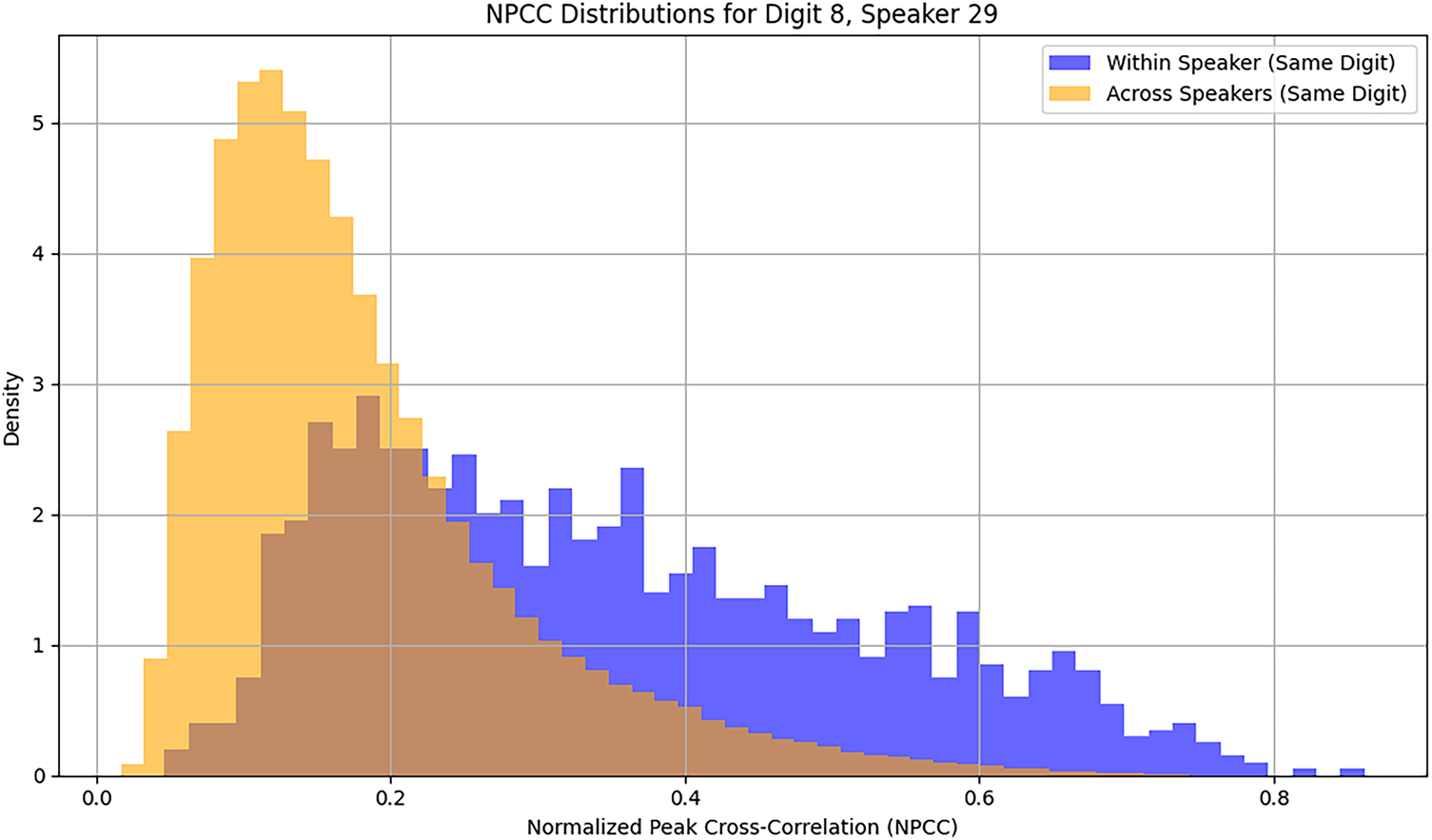
Figure 1: Distributions of NPCCs related to the audio recordings of digit-8 spoken by speaker-29. The blue histogram represents the within-speaker NPCCs, the light-brown histogram represents the cross-speaker NPCCs. The overlap between two histograms is shown in dark brown.

In Fig. 2, each of the four sets of figures shows the within-class (same speaker) and cross-class (different speakers) distributions of NPCCs for a particular digit spoken by a specific speaker. Each blue plot represents the distribution of 1,225 within-class NPCCs, and each light-brown plot represents the distribution of 29,500 cross-class NPCCS. For each case, as expected, the within-class NPCCs have greater values than cross-class NPCCs. The plots of Fig. 2 show there are virtually no similarities among the recitations of the same digit by different speakers.

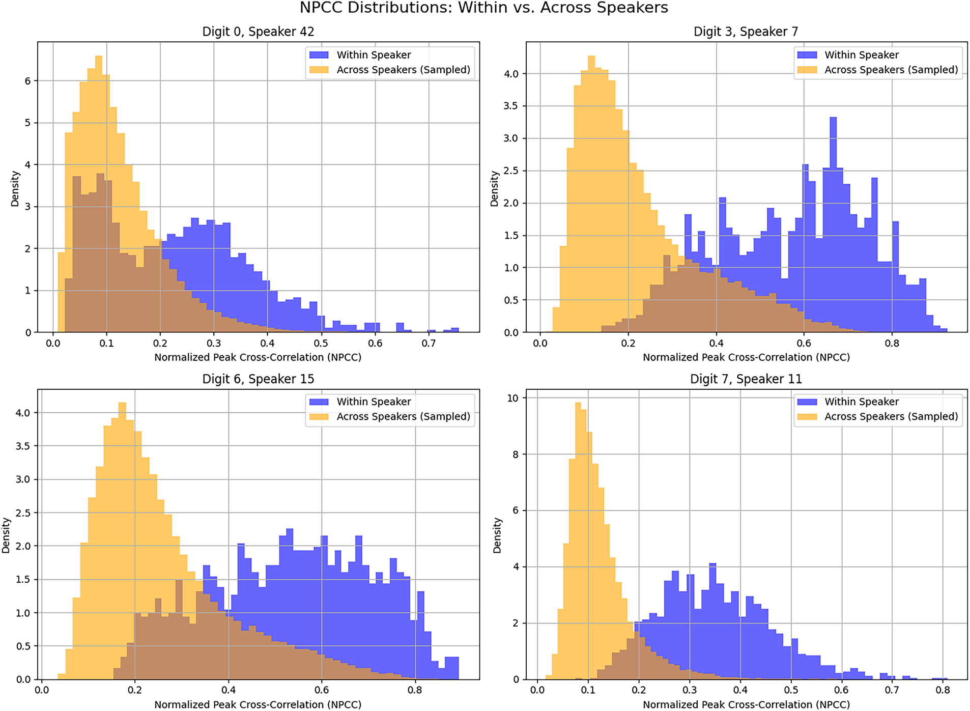
Figure 2: Distributions of NPCCs related to four different digit-speaker pairs. Each subplot compares the within-speaker NPCCs of one digit (blue, 1225 NPCC pairs) with the cross-speaker NPCCs of the same digit (light-brown, 29,500 NPCC pairs). Overlap is shown in dark brown.

The plots of Fig. 3 show the within-digit and cross-digit distributions of NPCCs for digit-9 spoken by speaker-13. The distribution of NPCCs of 1225 unique pairings of 50 recitations of the digit is shown in blue (within-digit). The distribution of NPCCs of 22,500 unique pairings of 50 recitations of digit-9 and 450 recitations of the remaining nine digits by the same speaker is shown in light brown (cross-digit). The overlap between distributions is shown in dark brown. The plots of Fig. 3 show that there is very little distinction between within-digit and cross-digit NPCCs. Considering the recitations of digits by the same speaker, the within-digit vagaries are as great as the cross-digit vagaries. These results point to the unfeasibility of utilizing NPCC for the classification of different digits spoken by the same speaker.

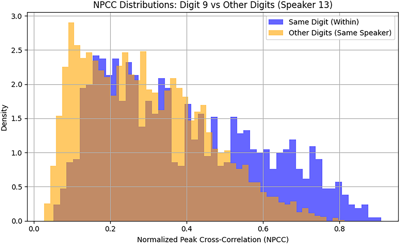
Figure 3: Distributions of NPCCs related to digit-9 spoken by speaker-13. The blue plot represents the within-digit histogram of NPCCs. The light-brown histogram shows NPCCs of 50 recitations of digit-9 and 450 recitations of the remaining nine digits by the same speaker.

To assess both the acoustic consistency and distinctiveness of digit pronunciations, we analyze three distributions of NPCCs centered around digit-7 spoken by speaker-20, which we call the target signal. These comparisons provide insight into how stable the articulation of a digit is when repeated by the same speaker, how similar it is when spoken by others, and how distinguishable it is from other digits across different voices.

Specifically, Fig. 4 plots the following three distributions. Same digit and same speaker, considers all 1225 pairwise NPCCs among the 50 recitations of the target signal. This distribution captures the intra-speaker consistency as well as vagary for a single digit. Same digit and other speakers, considers the NPCCs between the 50 utterances of the target signal and ten randomly selected utterances of digit-7 by each of the other 59 speakers totaling 29,500 comparisons. This distribution measures inter-speaker variability for the same digit. Other digits and other speakers which considers the NPCCs between the 50 utterances of the target signal and two randomly selected utterances of each of the other 9 digits by each of the 59 remaining speakers, totaling 53,100 comparisons. This distribution quantifies acoustic distinctiveness between digit-7 and other digits across the speaker population. By comparing these distributions, we can evaluate how reliably a digit is reproduced by a speaker, how consistent it is across speakers, and how distinct it is from other digits.

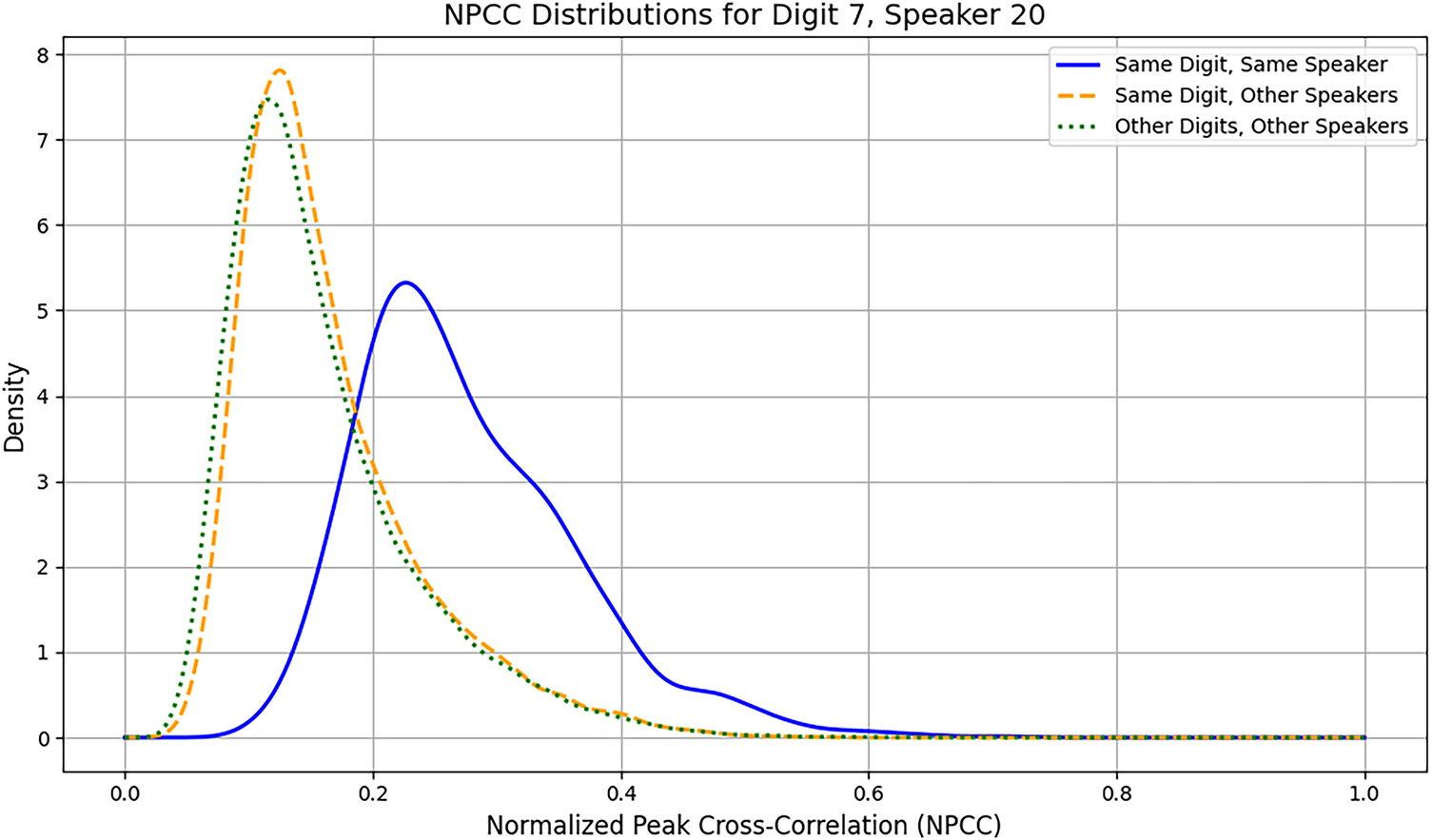
Figure 4: Distributions of NPCCs related to digit-7 spoken by speaker-20 (target signals). The solid line represents all pairwise NPCCs among 50 utterances of the target digit by the target speaker. The dashed line shows NPCCs between 50 recitations of the target signal and 590 recitations of the target digit by the remaining 59 speakers. The dotted line shows NPCCs of 50 target signals and the 1062 recitations of the remaining nine digits by the remaining 59 speakers.

The plots of Fig. 4 show that there is virtually no consistency between the recitations of the same digit across speakers. The great overlap between the dashed and dotted lines shows that the distribution of NPCCs of the target-digit recited by the target-speaker with respect to target-digit recited by other speakers, is virtually the same as the target-digit recited by the target-speaker with respect to other digits recited by other speakers. Therefore, NPCC is not a viable metric for classification of spoken digits.

Fig. 5 shows NPCC distribution comparisons across four different sets of digit and speaker combinations. Each set of tripartite distributions show the following: (1) The distribution of 1225 NPCCs corresponding to 50 recitations of the target digit by the target speaker (same digit and same speaker); (2) The distribution of 29,500 NPCCs corresponding to 50 recitations of the target digit by the target speaker with respect to ten randomly selected samples of the target digit spoken by each of the 59 remaining speakers (same digit and different speakers); (3) The distribution of 53,100 NPCCs corresponding to 50 recitations of the target digit by the target speaker with respect to two randomly selected samples of each of the other nine digits spoken by each of the 59 remaining speakers (different digits and different speakers).

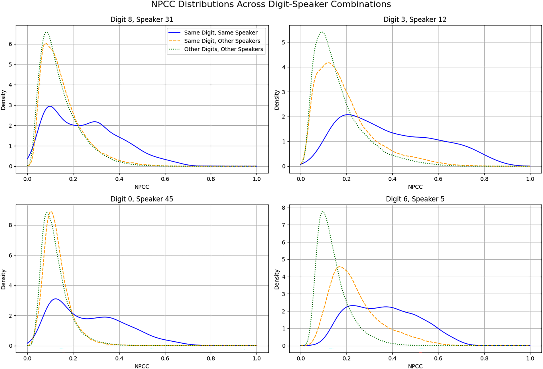
Figure 5: Distributions of NPCC values of four sets of digit-speaker pairs and comparisons with respect to same-digit spoken by other speakers, and other-digits spoken by other speakers.

The plots of Fig. 5 show that the distribution of NPCCs of the target digit with respect to the same digit spoken by different speakers is virtually indistinguishable from the NPCC values of target digit with respect to the other digits spoken by different speakers. The results constitute a quantitative validation of the long-held intuition that template-matching and matched-filter methodologies are inherently inadequate for effective audio signal classification.

5  One-Dimensional Convolution Neural Network

One-dimensional convolutional neural networks (1D-CNNs) process input audio signals by operating directly on the raw time-domain samples. Through a series of 1D convolution and max-pooling operations, these networks extract hierarchical features from the temporal structure of the signal [16,49,50]. The resulting feature representations are then passed to a fully connected feedforward (FCFF) block followed by a soft-max layer for classification into one of ten predefined classes.

The 1D-CNN classifier, as depicted in Fig. 6, is comprised of a sequential architecture designed for time-series data. The network begins with three convolutional layers, each paired with a max-pooling layer of size 2. All convolutional layers use the rectified linear unit (ReLU) as their activation function. Specifically, the first, second, and third CNN layers are configured with, respectively, 16, 32, and 64 filters, with corresponding filter sizes of 9, 7, and 5. Following the final max-pooling operation, a flatten layer converts the 3D feature maps into a 1D vector. This is then fed into a fully connected feedforward layer with 128 nodes and ReLU activation. The network concludes with an output layer containing 10 nodes, each with a sigmoid activation function, representing ten classes corresponding to spoken digits zero through nine. The input to this classifier is an 8000-element vector representing the time-domain samples of a single audio recording. The total number of trainable parameters for this architecture is 8,172,810.

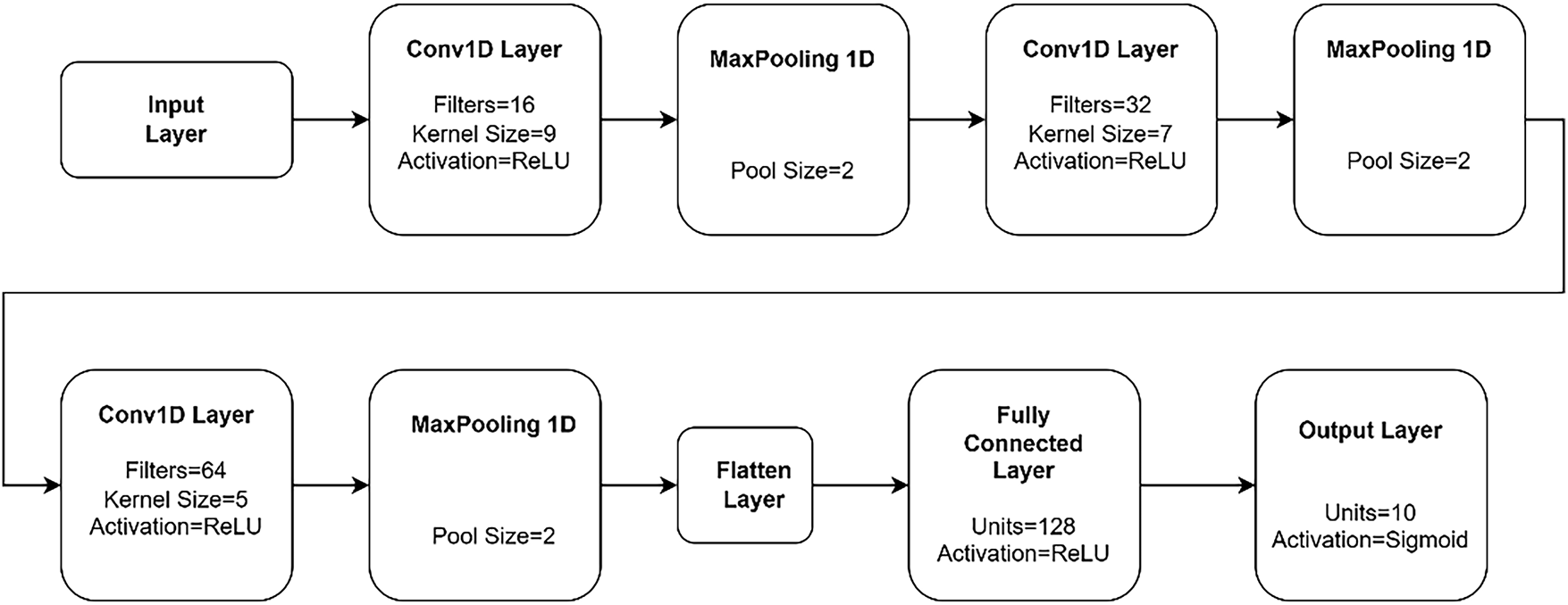
Figure 6: One-dimensional convolutional neural network (1D-CNN) classifier with three CNN and one FCFF layers.

The Audio-MNIST dataset described in Section 3 is used for training the classifier and evaluating the performance of the trained classifier. The classifier evaluation metric is the classification accuracy. The overall accuracy denotes the proportion of digits in the test set which are classified correctly. The per-digit accuracy denotes the proportion of each digit in the test set that is classified correctly.

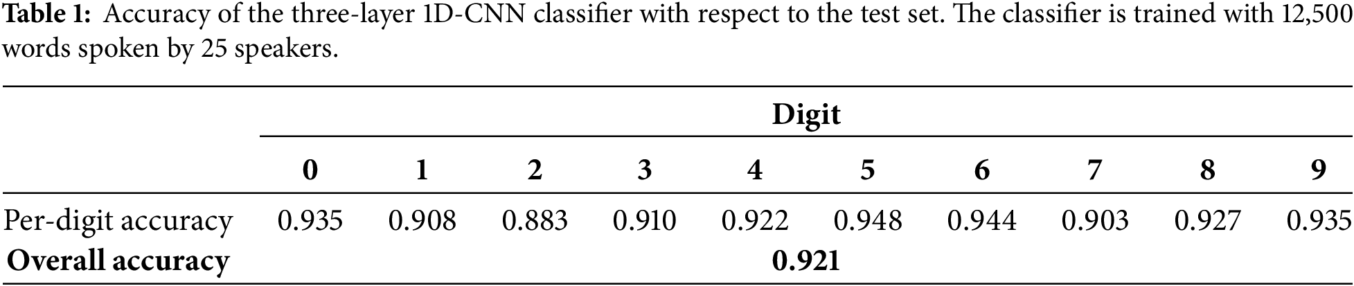
The classifier was trained using 12,500 digits spoken by 25 speakers randomly selected from the original set of 60. The 2500 digits spoken by five speakers randomly selected from the remaining 35 were used for validation. The test set comprises all 15,000 digits spoken by the remaining thirty speakers. It is noted that throughout the training process the classifier is not exposed to the validation and test sets.

The number of training epochs was set at 20 and the batch size was set at 64. The plots of Fig. 7 show the training history, where the classifier accuracy with respect to the training and validation data are shown at the end of each training epoch. It is seen that the classifier achieves accuracy of one with respect to the training set. The best performance with respect to the validation data was achieved at the conclusion of the sixteenth training epoch, with validation accuracy of 0.898, which means 89.8% of the validation digits are classified correctly.

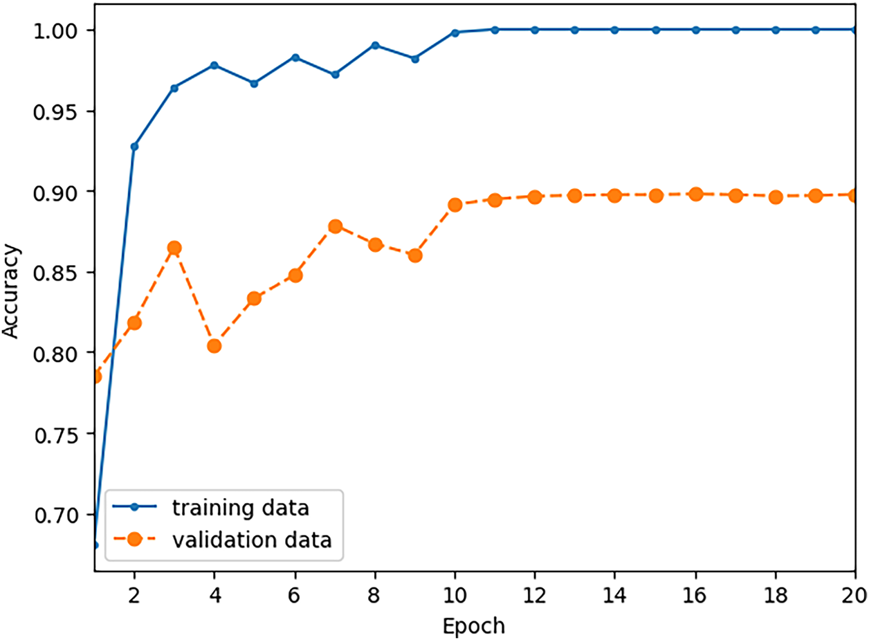
Figure 7: Training history of the 1D-CNN shows the accuracy of the classifier with respect to the training and validation data at the conclusion of each training epoch. The classifier is trained with 12,500 words spoken by 25 speakers.

The best performing model with respect to the validation data was saved and its performance with respect to the test set was evaluated. Table 1 lists the accuracy of the trained model with respect to the test data. Both the overall accuracy and the per-digit accuracy of the trained model are listed in Table 1.

The training and evaluation of the classifier of Fig. 6 was repeated using different sets of training, validation, and testing data compared to the previous case. This time the classifier was trained using 10,000 digits spoken by 20 speakers randomly selected from the original set of 60. For validation we used 5000 digits spoken by ten speakers randomly selected from the remaining 40. The test set comprises 15,000 digits spoken by the remaining thirty speakers. As before, the number of training epochs was 20 and the batch size was 64. The training history plots of Fig. 8 show the classifier accuracy with respect to the training and validation data at the end of each training epoch. It is seen that the classifier achieves accuracy of one with respect to the training set. The best performance with respect to the validation data was achieved at the conclusion of the nineteenth training epoch, with validation accuracy of 0.934.

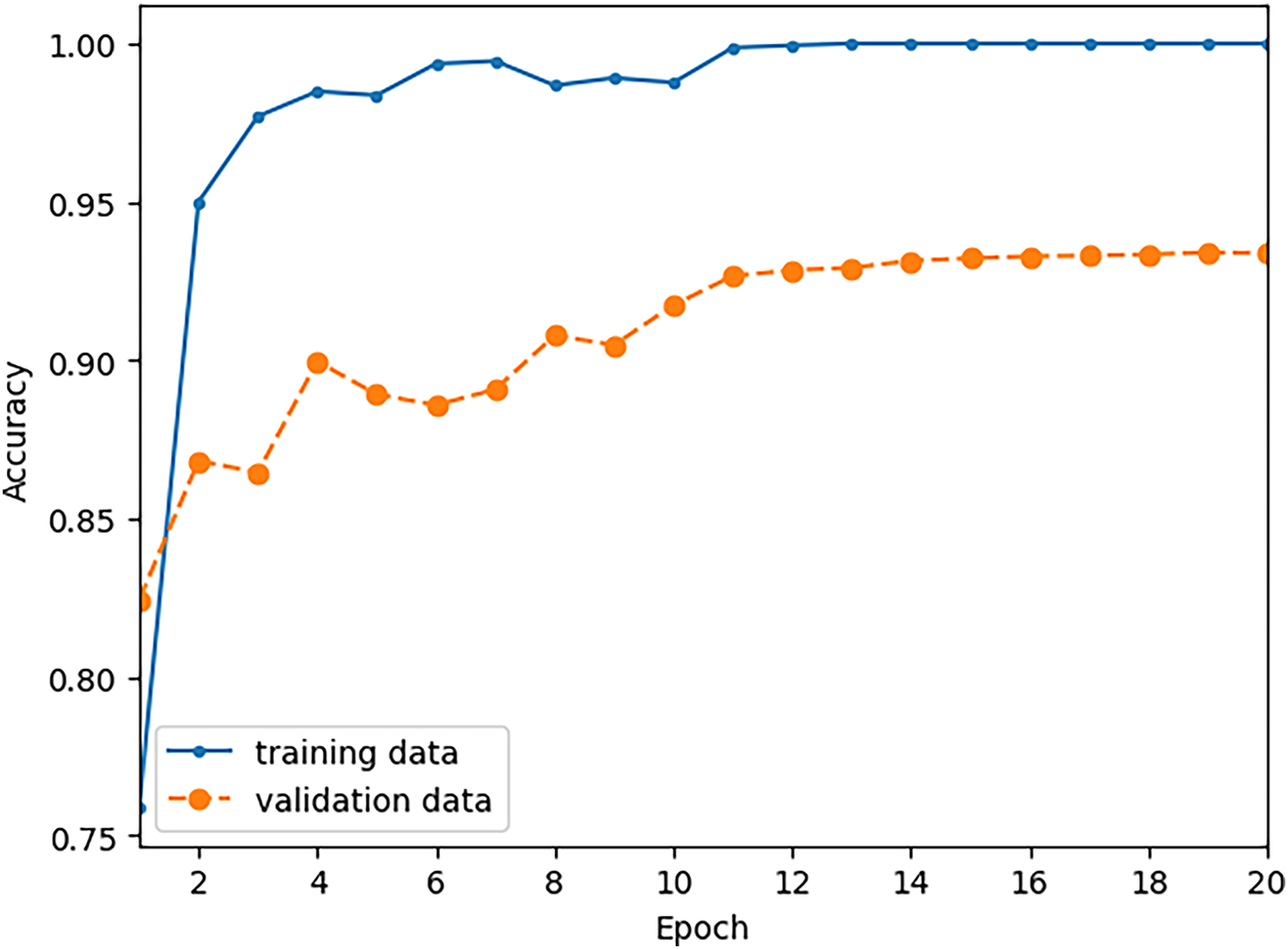
Figure 8: Training history of the 1D-CNN classifier shows the accuracy of the classifier with respect to the training and validation data at the conclusion of each training epoch. The classifier is trained with 10,000 words spoken by 20 speakers.

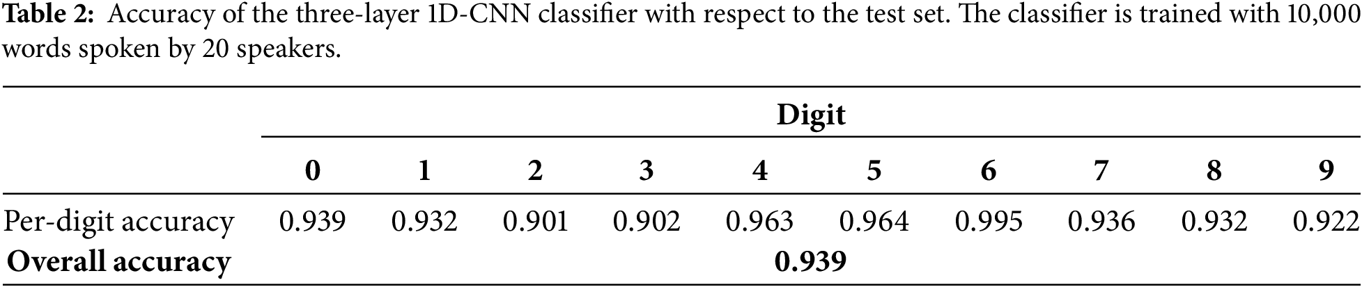
The best performing model with respect to the validation data was saved, and its performance with respect to the test set was evaluated. Table 2 lists the accuracy of the trained model with respect to the test data.

Analysis of the overall accuracy values presented in Tables 1 and 2 reveals an entirely counterintuitive result. It is noted that a slight improvement in classifier performance occurred when the number of trainer-set speakers was lowered from 25 to 20. This unexpected outcome, which should not be generalized, can be attributed to various factors. Foremost among these is the distinct random selection of training and validation speakers used in the two experiments. Specifically, the accents and speaking styles of the speakers chosen for the second experiment (Table 2) may have provided a more representative and effective training set for classifier as compared to those in the first experiment (Table 1).

Next, we investigate the variability in the trained classifier’s per-digit and overall accuracies with respect to the specific choices of the training, validation, and test datasets. The classifier architecture remains identical to the one shown in Fig. 6. The experiment is repeated ten times. In each iteration, a contiguous block of thirty speakers is selected to form the combined training and validation sets, with the remaining speakers serving as the test set. For these experiments, the number of speakers for the training, validation, and test sets are fixed at twenty, ten, and thirty, respectively. The starting point of the 30-speaker block is shifted by six speakers in each successive iteration. Within each experiment, twenty speakers are randomly chosen for training from the thirty-speaker block, and the remaining ten are used for validation. The resulting ten-fold performance, showing the per-digit and overall accuracies across all ten iterations, is presented in the box plots of Fig. 9. It is seen that this classifier has the lowest and the highest accuracies with respect to digits three and six, respectively.

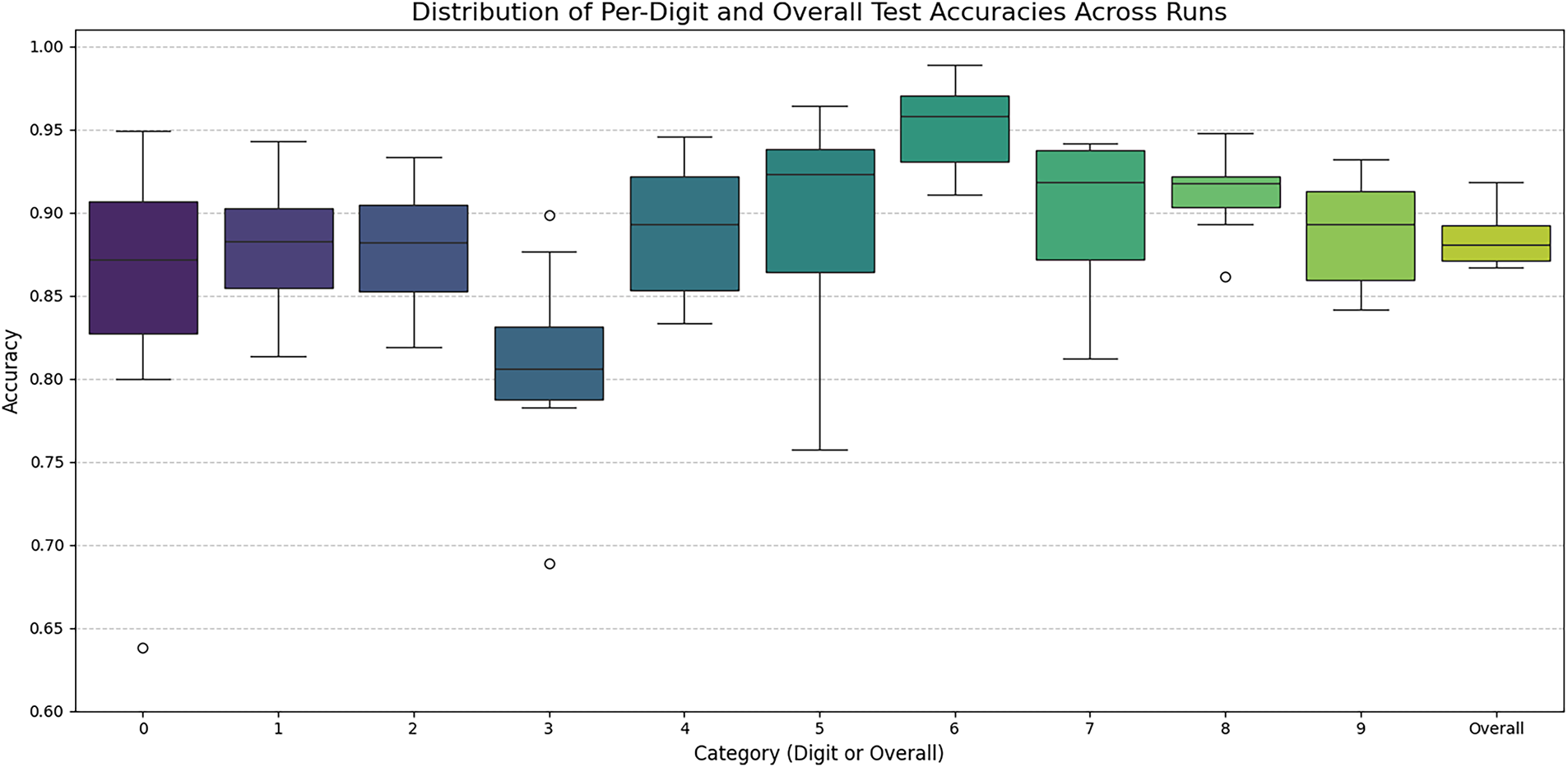
Figure 9: Distributions of per-digit and overall accuracies of the 1D-CNN classifier with three CNN layers across ten iterations of the training-validation-evaluation rounds. The overall accuracies are shown on the right side.

Next, we perform a more systemic investigation of the effect of the number of training set speakers on the classifier performance. The classifier is identical to the one shown in Fig. 6. For each setting of the number of speakers in the training set the experiment is repeated 25 times, where each iteration involves using different sets of speakers for training and testing. The classifier is trained using the training set, the performance of the trained classifier is evaluated using the test set, and the accuracy results are recorded. In each iteration of the experiment the classifier accuracy is evaluated using overall accuracy, and accuracy with respect to each digit.

Ten speakers are randomly chosen as the validation speakers. These speakers and the 5000 words spoken by them are set aside as the validation test set. The remaining fifty speakers are used as the combined training and test sets. For each setting of the number of training speakers, the trainer-set speakers are chosen randomly from the set of fifty, and the remaining speakers are used as the test set. The classifier is trained with the words spoken by the trainer-set speakers using twenty training epochs. The best performing classifier with respect to the words spoken by the validation-set speakers is saved as the trained model. The performance of the trained model is evaluated using the words spoken by the test-set speakers.

The boxplot of Fig. 10 shows the effect of the number of speakers in the training set on the classifier performance. For each setting of the number of speakers in the training set, the distribution of accuracies of the trained model with respect to all the spoken words in the test set are shown across 25 iterations of the experiment. It is noted that the overall accuracy of the trained model generally increases with increasing number of speakers in the training set.

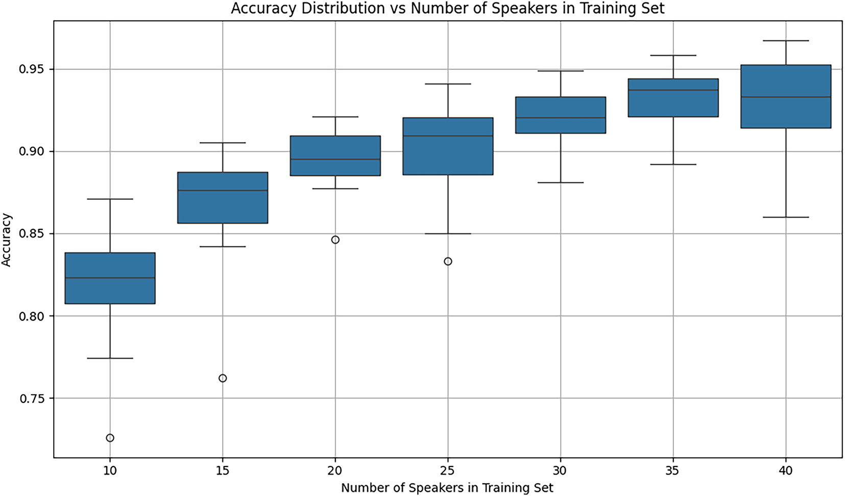
Figure 10: The effect of the number of speakers in the training set on the distributions of overall accuracies for the 1D-CNN classifier with three CNN layers.

It is also seen that there is a slight dip in accuracy when the number of speakers in the training set is increased from 35 to 40. This is due to the random selection process and should not be generalized. The mean accuracies of the trained classifier for 10 and 35 speakers in the training set are 0.817 and 0.932, respectively.

The plots of Fig. 11 show the effect of the number of speakers in the training set on the per-digit accuracies of the trained model. These plots show the average accuracies across 25 iterations of the experiment for each setting of the number of speakers in the training set. It is seen that with the training set comprised of ten speakers, the trained model has the lowest and highest accuracies with respect to digits three and six, respectively, where the mean accuracies for those digits are, respectively, 0.68 and 0.909. Similarly, with the training set comprised of forty speakers, the trained model has the lowest and highest accuracies with respect to digits three and six, respectively, where the mean accuracies for those digits are, respectively, 0.861 and 0.967.

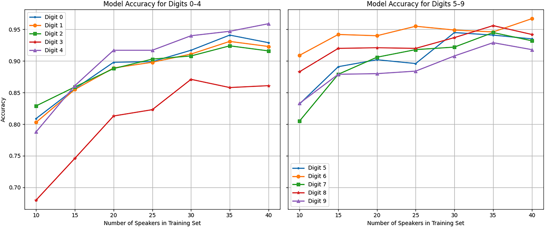
Figure 11: The effect of the number of speakers in the training set on the per-digit accuracies of the 1D-CNN classifier with three CNN layers.

Next, we investigate the performance of a 1D CNN classifier with five convolution layers similar to the one shown in Fig. 6. The new classifier comprises five CNN layers, where the number of filters for each layer is, respectively, 16, 32, 64, 128, 256, and the filters for all five layers are size 3. Each CNN layer is followed by a max-pooling layer with a size of two. The CNN-max-pooling block is followed by two fully connected feedforward (FCFF) layers with 128 and 64 nodes, and an output layer with ten nodes. The total number of trainable parameters of the classifier is 8,332,138, including 131,104 convolution parameters, and 8,201,034 feedforward parameters. The process of training this classifier and evaluating its performance is described below.

Ten speakers were set aside, and their 5000 words were used as the validation dataset. The validation speakers were identical to the speakers used for validation in the three-layer CNN described before. In each iteration of the experiment, forty speakers are randomly chosen from the remaining fifty speakers, and the corresponding 20,000 spoken words were used to train the classifier using fifty training epochs. The remaining ten speakers are used to evaluate the performance of the trained model. The process of random selection of the training speakers, training the model, and evaluating the performance of the trained model using the test speakers was repeated thirty times. The box plots of Fig. 12 show the thirty-fold performance results, where the per-digit and the overall accuracies are shown across thirty iterations of the experiment. The mean value of overall accuracies is 0.965, and the lowest mean accuracy is with respect to digit three at 0.928.

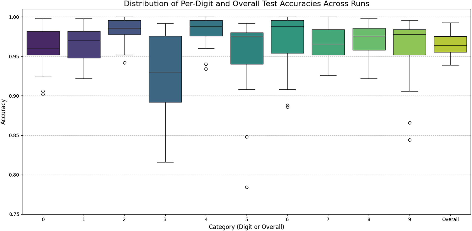
Figure 12: Distributions of per-digit and overall accuracies for a five-layer 1D-CNN classifier trained with 20,000 words spoken by forty speakers across 30 iterations of the training-validation-evaluation rounds. The mean value of overall accuracies is 0.965.

6  Two-Dimensional Convolution Neural Network

A two-dimensional convolutional neural network (2D-CNN) processes audio signals by operating on their 2D spectrograms. A spectrogram is a visual representation of the spectrum of frequencies of a signal as it changes over time. It provides a temporal-frequency representation of the one-channel (mono) audio signal, converting the 1D time-series data into a 2D image-like format suitable for 2D-CNNs.

6.1 Short-Time Fourier Transform (STFT)

The creation of a spectrogram begins with computing the short-time Fourier transform (STFT). This leads to localizing a signal in both the time and frequency domains simultaneously. The process of computing the STFT proceeds as follows:

a. Temporal Windowing: The 1D audio signal is first partitioned into a series of consecutive and partially overlapping temporal windows. The size of the window and the hop-size (the distance between the start of consecutive windows) are user-defined parameters. For the dataset used in this study (see Section 3), each audio signal contains 8,000 samples. With window-size of 1,024 and hop-size of 64 samples, each audio signal is partitioned into 126 windowed time-series.

b. Discrete Fourier Transform (DFT): The Discrete Fourier Transform (DFT) is then computed for each of the windowed time-series in part-a. The DFT of each window represents the frequency content of the original audio signal during specific temporal segment corresponding to the window.

c. Frequency and Sampling Rate: The number of frequency components in each DFT is determined by the number of time-samples in the corresponding temporal window. For the sampling rate of 8000 samples per second used in our dataset, the Nyquist criterion dictates that the maximum frequency that can be represented is 4 kHz. In our system, the number of time-samples in each window is set to 1024, which determines the resolution of the frequency spectrum for each time slice.

6.2 Spectrogram Construction

The final step of the spectrogram computation involves converting the STFT into a spectrogram. This process, often referred to as mel-spectrogram construction, is critical for audio classification tasks.

a. Magnitude and Phase: The STFT yields a complex-valued function. The phase information is typically discarded because it is less relevant for classification, and the squared absolute values (magnitudes) of the STFT are used. This results in an energy-based representation.

b. Mel-Frequency Bins: The human ear perceives frequencies on a non-linear scale. To mimic this, the linear frequency scale is converted to the mel-scale. The STFT magnitudes are binned into a user-prescribed number of mel-frequencies, which are logarithmically spaced. In our system, the number of mel-frequency bins is set to 128, distributed between 0 Hz (DC) and 4 kHz.

c. Final Mel-Spectrogram: By collating the mel-frequency binned magnitudes for each temporal window, a 2D array is formed. This array, with dimensions of 128 (mel-frequency bins) by 126 (temporal windows), is the final spectrogram. This 2D representation contains both the spectral (128 components) and temporal (126 components) information of the original audio signal, making it a suitable input for a 2D-CNN.

6.3 Dataset of Mel-Spectrograms

The set of 30,000 audio signals described in Section 3 is converted to the corresponding set of 2D mel-spectrograms, where each spectrogram has dimensions 128 × 126. Like the original audio signals, each spectrogram is labeled with the identity of the speaker reciting the word (0–59) and the spoken digit (0–9). The plots of Fig. 13 show a typical audio signal and the corresponding mel-spectrogram.

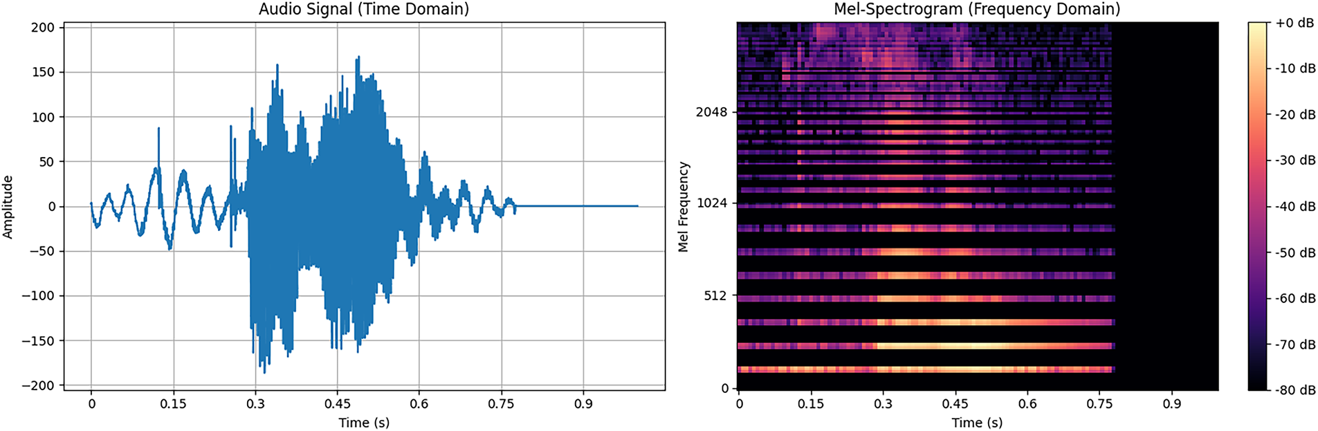
Figure 13: The audio signal (time-domain on left) and the corresponding mel-spectrogram of one recitation of digit-7 by speaker-56.

For training and performance evaluation of the classifier, the mel-spectrograms are normalized such that for each spectrogram the logarithms of pixel values are normalized to the [0–1] range. A subset of the 30,000 mel-spectrograms and the respective labels are used to train and validate a 2D-CNN classifier. The performance of the trained classifier is evaluated using the remaining mel-spectrograms.

6.4 Architecture of the 2D-CNN Classifier

The classifier architecture of the 2D-CNN used in this experiment is shown in Fig. 14. The classifier is comprised of five CNN layers, where the number of filters in layers one through five are, respectively, 32, 32, 64, 64, and 128. All the convolution filters have the same kernel size of 3 × 3. There are also three max-pooling layers with size 2 × 2, a flatten layer, and two feedforward fully connected (FC) layers with 256 and 64 nodes, respectively, and an output layer with ten nodes. The number of trainable parameters of this model is 8,020,522.

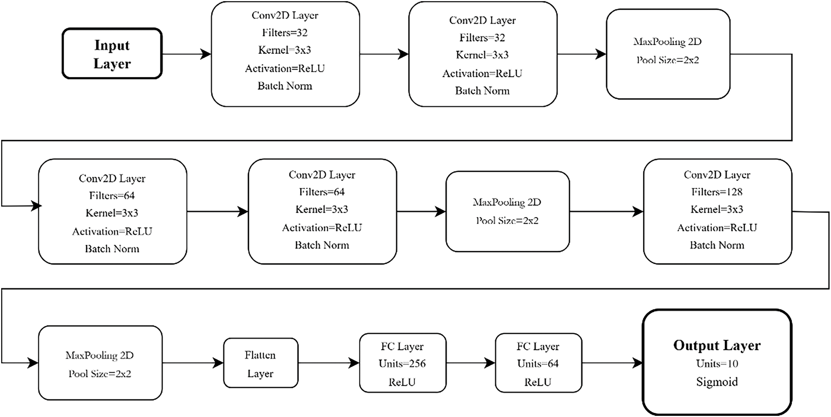
Figure 14: Two-dimensional convolutional neural network (2D-CNN) classifier with five CNN and two FC layers.

6.5 Training and Classification Results of the 2D-CNN Classifier

The spectrograms of 5000 words spoken by the first ten speakers (speakers 0 through 9) were set aside as the validation dataset. Forty of the remaining fifty speakers were chosen randomly, and 20,000 spectrograms of all the words recited by these speakers were used to train the classifier, using batch size of 64 and 50 training epochs. The plots of Fig. 15 show the training history, with classifier accuracy with respect to the training and validation data at the end of each training epoch. The classifier achieves accuracy of 0.9992 with respect to the training set. The best performance with respect to the validation data was achieved after 38 training epoch, with validation accuracy of 0.996, which means 99.6% of the validation digits (mel-spectrograms) are classified correctly. The best performing classifier with respect to the validation dataset was saved as the trained classifier.

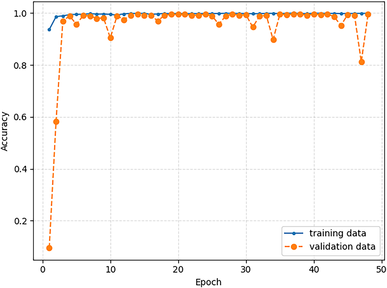
Figure 15: Training history of the 2D-CNN classifier trained with 20,000 mel-spectrograms of all the words spoken by forty speakers.

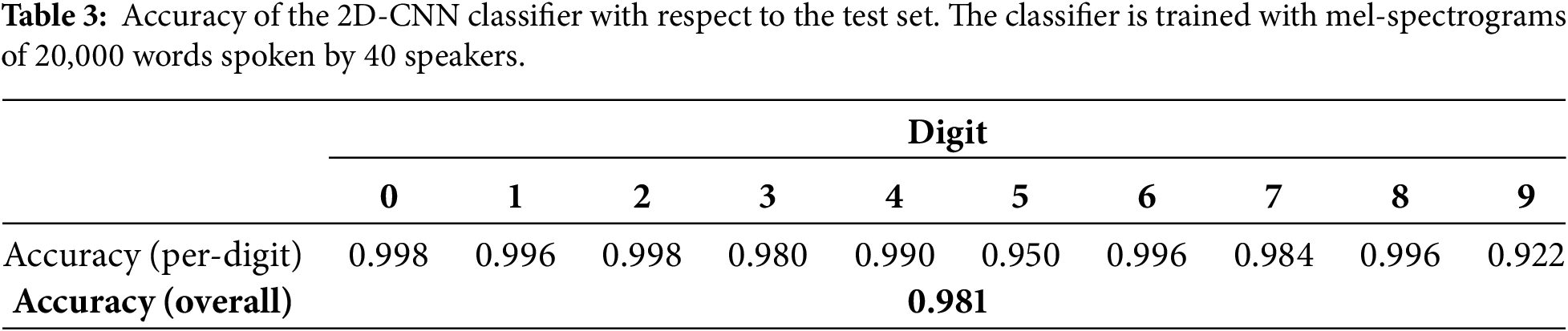
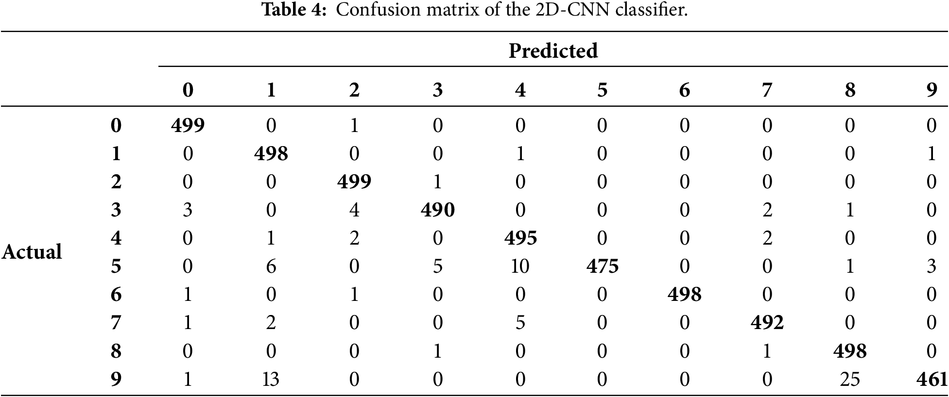
The trained classifier was used to label the mel-spectrograms of all the 5000 words recited by the remaining ten speakers. The performance of the trained classifier was assessed by comparing the labels predicted by the classifier with the true labels of each test spectrogram. Table 3 lists the overall and per-digit accuracies, and Table 4 shows confusion matrix of the trained classifier with respect to the test set. The numbers along the diagonal of the confusion matrix denote the number of correctly classified digits out of the 500 respective digits, and off-diagonal numbers denote the number of misclassified digits.

To assess the effects of the number and the composition of trainer-set speakers on the performance of the trained classifier, the number of speakers used to train the classifier was raised from ten to forty in steps of ten. As before, the 5000 words spoken by speakers zero through nine were set aside for validation. The trainer-set speakers is a contiguous set picked from the remaining fifty speakers, and the leftover speakers form the test set. For each setting of the number of trainer-set speakers, the experiment was repeated eleven times, each time moving the start of the trainer set block by four speakers.

Table 5 lists the per-digit and overall accuracies of the trained classifier averaged across eleven iterations of the experiment for each setting of the number of trainer-set speakers. Fig. 16 shows the range of overall accuracies of the classifier across eleven iterations of the experiment for each setting of the number of trainer-set speakers. As expected, the results of Table 5 and Fig. 16 show that overall accuracy, averaged across eleven iterations, increases as the number of trainer-set speakers is raised. This trend is also true for the per-digit accuracy for most of the ten digits.

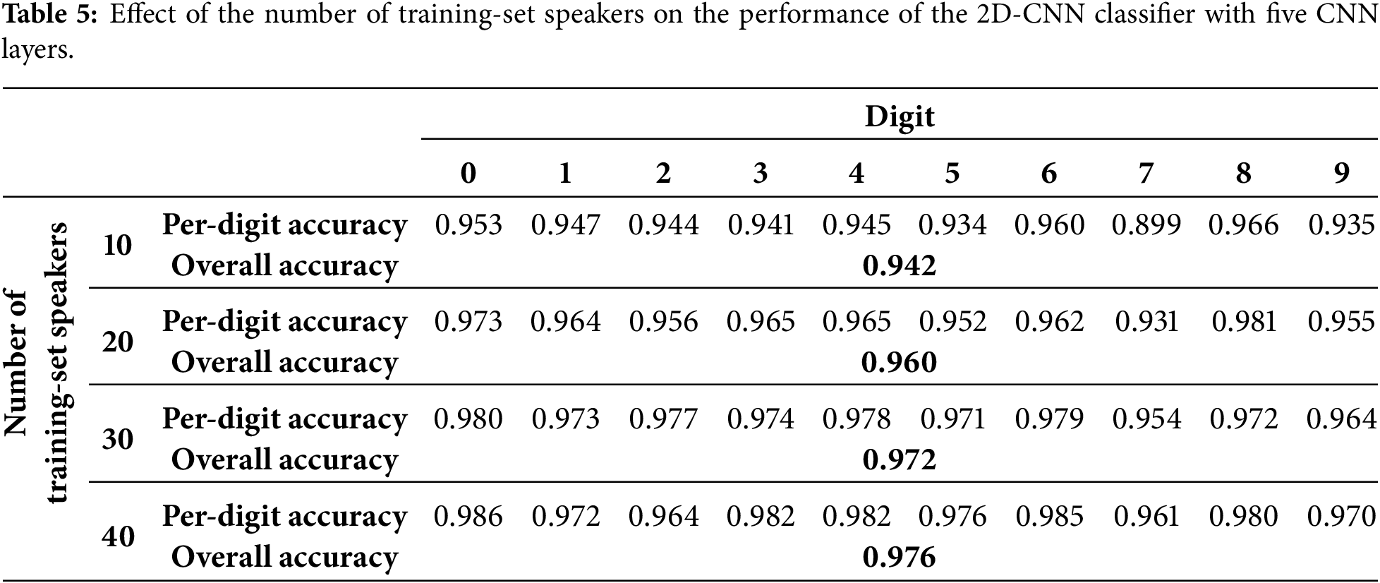
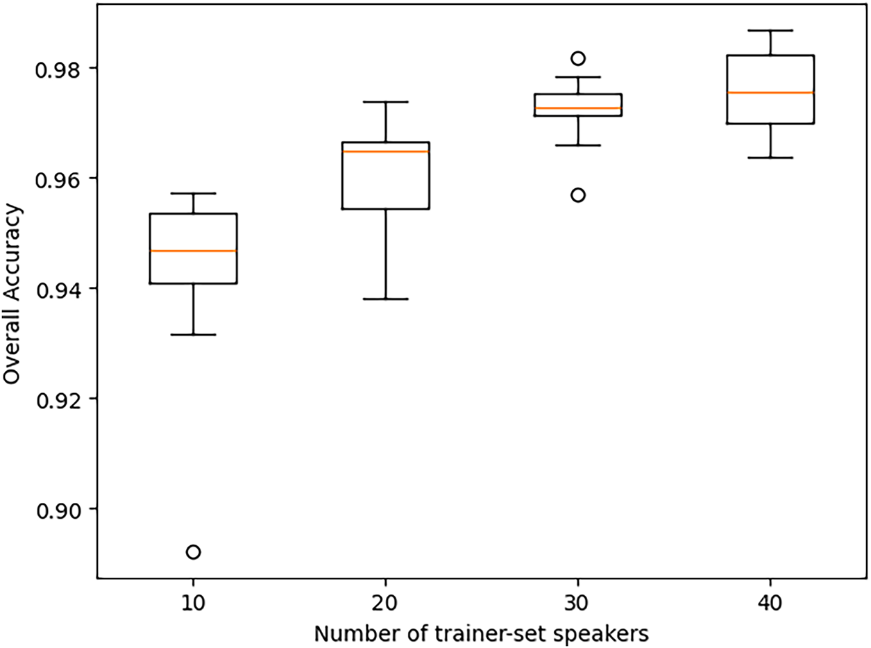
Figure 16: The effect of number of trainer-set speakers on the 2D-CNN classifier performance across eleven iterations of the experiment for each setting of the number of trainer-set speakers.

The performance results presented in Table 5 and Fig. 16, when compared with those in Section 5, demonstrate that 2D-CNN classifiers achieve superior performance metrics relative to 1D-CNN classifiers, while maintaining a comparable number of trainable parameters and similar inference complexity.

7  Comparison of CNN Classifiers with Whisper-AI

The performance of the 1D and 2D Convolutional Neural Network (CNN) models for spoken digit classification was compared against the performance of Whisper-AI.

Both CNN models were identically structured, each featuring five convolution layers and two fully connected layers, resulting in approximately 8 million trainable parameters. The models were trained and validated using data from fifty randomly selected speakers: forty speakers comprised the training set, and ten were used for validation. The performance metric used was the classification accuracy averaged across all digits in the test set. Classifiers were trained for 100 epochs, and the model exhibiting the best performance on the validation set was saved as the final trained classifier.

For the Whisper-AI evaluation, 6000 spoken digits were transcribed. This set comprised 600 randomly chosen recitations of each digit, distributed across all sixty speakers in the dataset. A dictionary of digit homophones was employed to map the model’s raw text transcriptions to the final digit classification.

Table 6 presents the per-digit and overall classification accuracies for the 1D-CNN, 2D-CNN, and Whisper-AI.

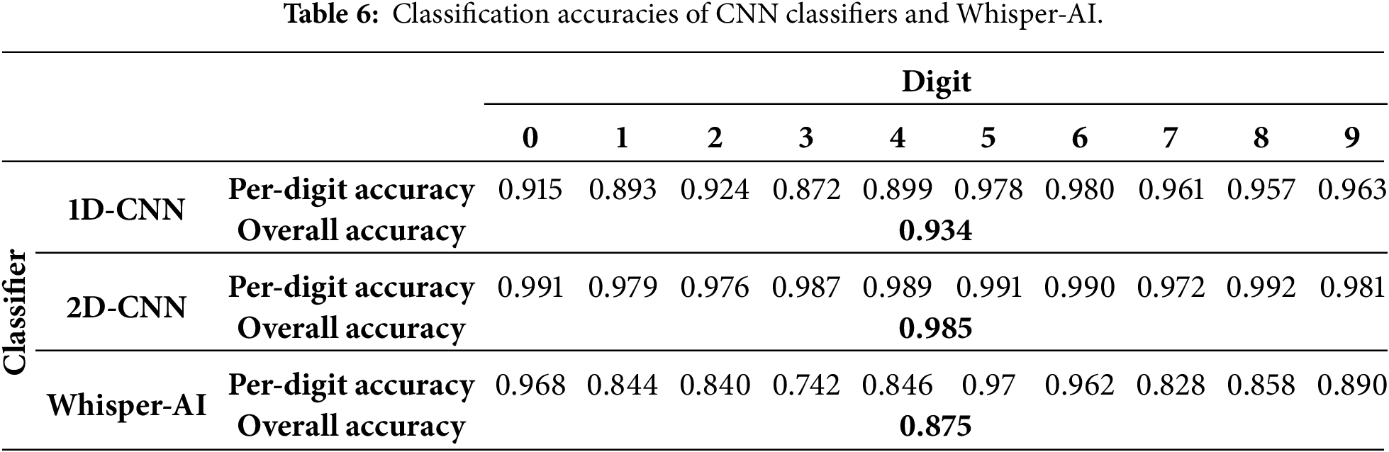
The results clearly indicate that the CNN classifiers outperform Whisper-AI. The 2D-CNN achieved the highest overall accuracy (0.985), significantly surpassing the 1D-CNN (0.934) and Whisper-AI (0.875). The lower performance of Whisper-AI is expected, as it is a general-purpose Automatic Speech Recognition (ASR) model designed for transcription in context, not optimized for isolated word (digit) classification. The classification process relies on a direct comparison between the transcribed text and a predefined list of digit homophones, which inherently introduces potential errors.

The classification accuracy of Whisper-AI could be substantially improved through two main methods:

1. Developing a more comprehensive dictionary of digit homophones to account for a wider variety of spellings and phonetic variations.

2. Applying common string distance metrics (e.g., Levenshtein distance) to forcibly map the transcription to one of the ten possible digit labels, thereby mitigating transcription errors that fall outside the current homophone dictionary.

8  Conclusions

In this study, we have successfully developed and analyzed two distinct Convolutional Neural Network (CNN) architectures, a 1D-CNN and a 2D-CNN, for the classification of isolated spoken words from a limited dictionary. The 1D-CNN directly processes the raw time-series audio signal, while the 2D-CNN operates on the Mel-spectrogram representation, leveraging its rich time-frequency features.

Using the open-source Audio-MNIST dataset, we conducted a thorough evaluation of both models. Our analysis systematically investigated the influence of key design choices on classification performance, including the comparison between 1D and 2D architectures, network depth, the number and size of convolutional filters, and the configuration of subsequent feedforward layers. The results demonstrated a clear advantage for the spectrogram-based 2D-CNN, which consistently achieved superior classification accuracy compared to the 1D-CNN when both models were matched for the number of trainable parameters.

A significant component of our research involved a comprehensive evaluation of speaker diversity. We studied the impact of the number of unique speakers included in the training set on the overall and per-digit classification accuracy. Furthermore, we assessed how performance metrics varied when the training, validation, and test sets comprised distinct speaker populations, providing valuable insights into the models’ generalization capability to unseen voices.

Finally, we compared the performance of our optimized CNN models against the Large Language Model (LLM) Whisper-AI. For the application of classifying isolated words out of context from a finite, predefined dictionary, the CNN classifiers exhibited better classification accuracy than Whisper-AI. This finding underscores the effectiveness of purpose-built, highly optimized CNN models for specific, limited-vocabulary tasks over general-purpose transcription LLMs.

In summary, this work highlights the superior performance of 2D-CNNs for isolated audio command recognition and provides key data on the impact of speaker diversity. Future work will concentrate on (i) investigating the role of synthetic data augmentation in enhancing classifier robustness and (ii) evaluating the impact of various types of background noise on classification accuracy.

Acknowledgement: Not applicable.

Funding Statement: Kaveh Heidary was partially supported by NSF through Grant #205154-20502-61008-140.

Availability of Data and Materials: The data that support the findings of this study are openly available in reference [48] at https://www.kaggle.com/datasets/sripaadsrinivasan/audio-mnist.

Ethics Approval: Not applicable.

Conflicts of Interest: The author declares no conflicts of interest to report.

References

1. Breebaart J, McKinney MF. Features for audio classification. In: Verhaegh WFJ, Aarts E, Korst J, editors. Algorithms in ambient intelligence. Philips research. Vol. 2. Dordrecht, The Netherlands: Springer; 2004. doi:10.1007/978-94-017-0703-9_6. [Google Scholar] [CrossRef]

2. Jarina R, Paralic M, Kuba M, Olajec J, Lukác A, Dzurek M. Development of a reference platform for generic audio classification. In: Proceedings of the 2008 Ninth International Workshop on Image Analysis for Multimedia Interactive Services; 2008 May 7–9; Klagenfurt, Austria. doi:10.1109/WIAMIS.2008.39. [Google Scholar] [CrossRef]

3. O’Shaughnessy D. Interacting with computers by voice: automatic speech recognition and synthesis. Proc IEEE. 2003;91(9):1272–305. doi:10.1109/jproc.2003.817117. [Google Scholar] [CrossRef]

4. Lin CC, Chen SH, Truong TK, Chang Y. Audio classification and categorization based on wavelets and support vector Machine. IEEE Trans Speech Audio Process. 2005;13(5):644–51. doi:10.1109/TSA.2005.851880. [Google Scholar] [CrossRef]

5. Qi J, Tejedor J. Classical-to-quantum transfer learning for spoken command recognition based on quantum neural networks. In: Proceedings of the ICASP 2022 IEEE International Conference on Acoustics, Speech, and Signal Processing; 2022 May 23–27; Singapore. doi:10.1109/icassp43922.2022.9747636. [Google Scholar] [CrossRef]

6. Bae J, Kim DS. End-to-end speech command recognition with capsule network. In: Interspeech 2018. Singapore: ISCA; 2018. p. 776–80. doi:10.21437/interspeech.2018-1888. [Google Scholar] [CrossRef]

7. Pervaiz A, Hussain F, Israr H, Ali Tahir M, Raja FR, Baloch NK, et al. Incorporating noise robustness in speech command recognition by noise augmentation of training data. Sensors. 2020;20(8):2326. doi:10.3390/s20082326. [Google Scholar] [PubMed] [CrossRef]

8. Zhang SX, Zhao R, Liu C, Li J, Gong Y. Recurrent support vector machines for speech recognition. In: Proceedings of the 2016 IEEE International Conference on Acoustics, Speech and Signal Processing (ICASSP); 2016 Mar 20–25; Shanghai, China. doi:10.1109/ICASSP.2016.7472806. [Google Scholar] [CrossRef]

9. Raiaan MAK, Mukta MSH, Fatema K, Fahad NM, Sakib S, Mim MMJ, et al. A review on large language models: architectures, applications, taxonomies, open issues and challenges. IEEE Access. 2024;12(8):26839–74. doi:10.1109/access.2024.3365742. [Google Scholar] [CrossRef]

10. Bengio Y, Ducharme R, Vincent P, Janvin C. A neural probabilistic language model. J Mach Learn Res. 2003;3:1137–55. [Google Scholar]

11. Rosenfeld R. Two decades of statistical language modeling: where do we go from here? Proc IEEE. 2000;88(8):1270–8. doi:10.1109/5.880083. [Google Scholar] [CrossRef]

12. Open AI [Internet]. 2022 [cited 2025 Dec 3]. Available from: https://openai.com/index/whisper/. [Google Scholar]

13. Peng J, Wang Y, Li B, Guo Y, Wang H, Fang Y, et al. A survey on speech large language models for understanding. arXiv:2410.18908. 2024. [Google Scholar]

14. Cui W, Yu D, Jiao X, Meng Z, Zhang G, Wang Q, et al. Recent advances in speech language models: a survey. arXiv:2410.03751. 2024. [Google Scholar]

15. Ahlawat H, Aggarwal N, Gupta D. Automatic speech recognition: a survey of deep learning techniques and approaches. Int J Cogn Comput Eng. 2025;6(7):201–37. doi:10.1016/j.ijcce.2024.12.007. [Google Scholar] [CrossRef]

16. Li Z, Liu F, Yang W, Peng S, Zhou J. A survey of convolutional neural networks: analysis, applications, and prospects. IEEE Trans Neural Netw Learning Syst. 2022;33(12):6999–7019. doi:10.1109/tnnls.2021.3084827. [Google Scholar] [PubMed] [CrossRef]

17. Aloysius N, Geetha M. A review on deep convolutional neural networks. In: Proceedings of the 2017 International Conference on Communication and Signal Processing (ICCSP); 2017 Apr 6–8; Chennai, India. doi:10.1109/ICCSP.2017.8286426. [Google Scholar] [CrossRef]

18. Zhao X, Wang L, Zhang Y, Han X, Deveci M, Parmar M. A review of convolutional neural networks in computer vision. Artif Intell Rev. 2024;57(4):99. doi:10.1007/s10462-024-10721-6. [Google Scholar] [CrossRef]

19. Gilbert AC, Strauss MJ, Tropp JA. A tutorial on fast Fourier sampling. IEEE Signal Process Mag. 2008;25(2):57–66. doi:10.1109/msp.2007.915000. [Google Scholar] [CrossRef]

20. Oppenheim AV, Schafer RW. Discrete-time signal processing. Harlow, UK: Pearson; 2014. p. 880–4. [Google Scholar]

21. Boashash B. Estimating and interpreting the instantaneous frequency of a signal. Proc IEEE. 1992;80(4):520–38. doi:10.1109/5.135376. [Google Scholar] [CrossRef]

22. Hoy MB. Alexa, Siri, Cortana, and more: an introduction to voice assistants. Med Ref Serv Q. 2018;37(1):81–8. doi:10.1080/02763869.2018.1404391. [Google Scholar] [PubMed] [CrossRef]

23. Chittepu S, Martha S, Banik D. Empowering voice assistants with TinyML for user-centric innovations and real-world applications. Sci Rep. 2025;15(1):15411. doi:10.1038/s41598-025-96588-1. [Google Scholar] [PubMed] [CrossRef]

24. Hong G, Folcarelli A, Less J, Wang C, Erbasi N, Lin S. Voice assistants and cancer screening: a comparison of Alexa, Siri, Google Assistant, and Cortana. Ann Fam Med. 2021;19(5):447–9. doi:10.1370/afm.2713. [Google Scholar] [PubMed] [CrossRef]

25. Lachenani S, Kheddar H, Ouldzmirli M. Improving pretrained YAMNet for enhanced speech command detection via transfer learning. In: Proceedings of the 2024 International Conference on Telecommunications and Intelligent Systems (ICTIS); 2024 Dec 14–15; Djelfa, Algeria. doi:10.1109/ICTIS62692.2024.10894266. [Google Scholar] [CrossRef]

26. Mesaros A, Heittola T, Virtanen T, Plumbley MD. Sound event detection: a tutorial. IEEE Signal Process Mag. 2021;38(5):67–83. doi:10.1109/msp.2021.3090678. [Google Scholar] [CrossRef]

27. Chu S, Narayanan S, Kuo CJ. Environmental sound recognition with time-frequency audio features. IEEE Trans Audio Speech Lang Process. 2009;17(6):1142–58. doi:10.1109/tasl.2009.2017438. [Google Scholar] [CrossRef]

28. Mu W, Yin B, Huang X, Xu J, Du Z. Environmental sound classification using temporal-frequency attention based convolutional neural network. Sci Rep. 2021;11(1):21552. doi:10.1038/s41598-021-01045-4. [Google Scholar] [PubMed] [CrossRef]

29. Akbal E. An automated environmental sound classification methods based on statistical and textural feature. Appl Acoust. 2020;167(3):107413. doi:10.1016/j.apacoust.2020.107413. [Google Scholar] [CrossRef]

30. Barchiesi D, Giannoulis D, Stowell D, Plumbley MD. Acoustic scene classification: classifying environments from the sounds they produce. IEEE Signal Process Mag. 2015;32(3):16–34. doi:10.1109/MSP.2014.2326181. [Google Scholar] [CrossRef]

31. Bisot V, Serizel R, Essid S, Richard G. Feature learning with matrix factorization applied to acoustic scene classification. IEEE ACM Trans Audio Speech Lang Process. 2017;25(6):1216–29. doi:10.1109/TASLP.2017.2690570. [Google Scholar] [CrossRef]

32. Mushtaq Z, Su SF. Efficient classification of environmental sounds through multiple features aggregation and data enhancement techniques for spectrogram images. Symmetry. 2020;12(11):1822. doi:10.3390/sym12111822. [Google Scholar] [CrossRef]

33. Rabaoui A, Davy M, Rossignol S, Ellouze N. Using one-class SVMs and wavelets for audio surveillance. IEEE Trans Inf Forensics Secur. 2008;3(4):763–75. doi:10.1109/TIFS.2008.2008216. [Google Scholar] [CrossRef]

34. Sawant O, Bhowmick A, Bhagwat G. Separation of speech & music using temporal-spectral features and neural classifiers. Evol Intell. 2024;17(3):1389–403. doi:10.1007/s12065-023-00828-0. [Google Scholar] [CrossRef]

35. Albouy P, Mehr SA, Hoyer RS, Ginzburg J, Du Y, Zatorre RJ. Spectro-temporal acoustical markers differentiate speech from song across cultures. Nat Commun. 2024;15(1):4835. doi:10.1038/s41467-024-49040-3. [Google Scholar] [PubMed] [CrossRef]

36. Mirbeygi M, Mahabadi A, Ranjbar A. RPCA-based real-time speech and music separation method. Speech Commun. 2021;126(5):22–34. doi:10.1016/j.specom.2020.12.003. [Google Scholar] [CrossRef]

37. Alías F, Socoró J, Sevillano X. A review of physical and perceptual feature extraction techniques for speech, music and environmental sounds. Appl Sci. 2016;6(5):143. doi:10.3390/app6050143. [Google Scholar] [CrossRef]

38. Heittola T, Mesaros A, Eronen A, Virtanen T. Audio context recognition using audio event histograms. In: Proceedings of the 18th European Signal Processing Conference; 2010 Aug 23–27; Aalborg, Denmark. [Google Scholar]

39. Dargie W. Adaptive audio-based context recognition. IEEE Trans Syst Man Cybern Part A Syst Hum. 2009;39(4):715–25. doi:10.1109/tsmca.2009.2015676. [Google Scholar] [CrossRef]

40. Neuschmied H, Mayer H, Batlle E. Content-based identification of audio titles on the Internet. In: Proceedings of the First International Conference on WEB Delivering of Music WEDELMUSIC 2001; 2001 Nov 23–24; Florence, Italy. doi:10.1109/WDM.2001.990163. [Google Scholar] [CrossRef]

41. Atmaja BT, Sasou A. Sentiment analysis and emotion recognition from speech using universal speech representations. Sensors. 2022;22(17):6369. doi:10.3390/s22176369. [Google Scholar] [PubMed] [CrossRef]

42. Li B, Dimitriadis D, Stolcke A. Acoustic and lexical sentiment analysis for customer service calls. In: Proceedings of the ICASSP 2019–2019 IEEE International Conference on Acoustics, Speech and Signal Processing (ICASSP); 2019 May 12–17; Brighton, UK. doi:10.1109/ICASSP.2019.8683679. [Google Scholar] [CrossRef]

43. Tolstoukhov DE, Egorov DP, Verina YV, Kravchenko OV. Hybrid model for sentiment analysis based on both text and audio data. In: Sentimental analysis and deep learning. Berlin/Heidelberg, Germany: Springer; 2021. p. 993–1001. doi:10.1007/978-981-16-5157-1_77. [Google Scholar] [CrossRef]

44. Delvecchio S, Bonfiglio P, Pompoli F. Vibro-acoustic condition monitoring of internal combustion engines: a critical review of existing techniques. Mech Syst Signal Process. 2018;99(62–63):661–83. doi:10.1016/j.ymssp.2017.06.033. [Google Scholar] [CrossRef]

45. Wang YS, Liu NN, Guo H, Wang XL. An engine-fault-diagnosis system based on sound intensity analysis and wavelet packet pre-processing neural network. Eng Appl Artif Intell. 2020;94:103765. doi:10.1016/j.engappai.2020.103765. [Google Scholar] [CrossRef]

46. Bondarenko O, Fukuda T. Potential of acoustic emission in unsupervised monitoring of gas-fuelled engines. IFAC-PapersOnLine. 2016;49(23):329–34. doi:10.1016/j.ifacol.2016.10.425. [Google Scholar] [CrossRef]

47. Becker S, Vielhaben J, Ackermann M, Müller KR, Lapuschkin S, Samek W. AudioMNIST: exploring explainable artificial intelligence for audio analysis on a simple benchmark. J Frankl Inst. 2024;361(1):418–28. doi:10.1016/j.jfranklin.2023.11.038. [Google Scholar] [CrossRef]

48. Srinivasan S. Audio MNIST [Internet]. [cited 2025 Dec 3]. Available from: https://www.kaggle.com/datasets/sripaadsrinivasan/audio-mnist. [Google Scholar]

49. Voulodimos A, Doulamis N, Doulamis A, Protopapadakis E. Deep learning for computer vision: a brief review. Comput Intell Neurosci. 2018;2018:7068349. doi:10.1155/2018/7068349. [Google Scholar] [CrossRef]

50. Kiranyaz S, Ince T, Abdeljaber O, Avci O, Gabbouj M. 1-D convolutional neural networks for signal processing applications. In: Proceedings of the ICASSP 2019–2019 IEEE International Conference on Acoustics, Speech and Signal Processing (ICASSP); 2019 May 12–17; Brighton, UK. doi:10.1109/icassp.2019.8682194. [Google Scholar] [CrossRef]