Hybrid Model for Short-Term Passenger Flow Prediction in Rail Transit

1  Introduction

Rail transit efficiently reduces the burden of ground traffic, and it has the benefits of being fast and increasing land utilization. The accessible rail system has resulted in a massive influx of people. That, however, concealed security risks as well. To schedule operational resources, plan for corresponding safety emergency measures, and predict the passenger flow in advance.

Accurate real-time data on subway passenger flow serves multiple purposes. Firstly, it supports the operation and scheduling of the subway system, ensuring its effective functioning and enabling decision-making during major events or emergencies. Secondly, it helps the traffic management department better understand passenger flow patterns in advance, allowing them to allocate resources effectively and formulate emergency management measures. Accurate predictions of urban rail transit passenger flow are crucial in preventing safety accidents. Therefore, precise forecasting of rail transit passenger flow is vital for the future planning and development of rail transit routes [1].

Short-term passenger flow prediction typically utilizes time intervals of 15 min, 30 min, and 1 h. In terms of research methodology, there are three main focuses: prediction models based on mathematical statistics, intelligent algorithm prediction models, and hybrid models.

The prediction model based on mathematical approaches aims to discover inherent patterns within passenger flow data and achieve accurate predictions by leveraging mathematical relationships. Specifically, this approach involves using mathematical equations to analyze the patterns of variable changes based on available data. Commonly employed models include time series models, moving average models, and Kalman filter models. In short-term passenger flow prediction, Pan [2] confirmed the effectiveness of the time-series model. Additionally, Meng et al. [3] identified that subway passenger flow exhibits regularity within specific periods of each day, aligning with daily work and rest patterns. Accordingly, historical data can be effectively predicted using the moving average algorithm. Furthermore, Xiong et al. [4] viewed the subway transfer process as a dynamic system. They developed stochastic linear offline equations based on the Kalman filter to forecast passenger flow during rush hours on both working days and holidays.

In the field of rail transit safety, intelligent algorithms have been further developed and applied to short-term passenger flow prediction. Two main branches in this area are machine learning models [5,6] and neural networks [7–10]. Machine learning models differ from the principles of mathematical statistics and rely on supervised or unsupervised learning methods to extract important information from data and make predictions. Hu et al. [11] used Support Vector Machines (SVM) to build a regression model, demonstrating its higher accuracy and reliability. Roos et al. [12] incorporated passenger flow characteristics from adjacent space and time into their model and proposed a dynamic Bayesian network for real-time prediction. Li et al. [6] utilized the correlation between Gaussian Bayesian networks to predict microscopic traffic data.

Based on big data, machine learning methods have limitations, such as limited feature processing power. Neural networks [8,10,13] overcome these limitations by enabling large-batch computing and deep mining, making them the mainstream method for predicting passenger flow. Neural networks aim to learn complex features through a series of nonlinear transformations [14]. Wei et al. [15] employed empirical modal decomposition to extract intrinsic modal functions (IMFs) and introduced temporal characteristics to predict passenger flow. Li et al. [6] incorporated the relationship between passenger flow and train schedules, utilizing dynamic radial basis function (RBF) to forecast passenger flow. Gong et al. [16] recognized the strong memory capacity of LSTM in prediction tasks, addressing the issues of gradient explosion and model over-fitting. Ma et al. [17] leveraged CNN to predict traffic network speed on a large scale, organizing trajectory data from different road sections at different times as spatial and temporal matrices.

In the idea of integrated learning, model fusion [18–28] can effectively leverage the strengths of different models to extract valuable information. Bai et al. [19] utilized the Affinity Propagation (AP) algorithm to mine features and incorporated it into a hybrid model (DBN) for enhanced feature recognition and learning capabilities. Neural networks have also been recognized as fundamental models in model fusion, particularly for their strong feature extraction capabilities in the convolutional layer. Zhang [25] combined neural networks with time series models and iteratively updated the loss function. Zhang [21] employed the graph convolutional neural network to extract complex characteristics of available paths and subway station spaces, and combined it with the Gating Convolution (GLU) algorithm to explore time-varying traffic patterns caused by fluctuations. Through comparative analysis, it was found that the hybrid model exhibited high robustness. Peng et al. [24] combined GRU and LSTM to extract external features and continuously update the loss using a weighted square method. LSTM, compared to linear methods, excels at capturing the temporal properties of sequences and processing temporal features [29].

In the application of the above models for short-term passenger flow prediction, they are directly employed to predict passenger flow data without considering the exploration of hidden time information within the data. Furthermore, there is a lack of feature engineering from the perspective of the external objective environment and space-time. The external objective environment encompasses factors such as rush hour, weekends, air quality, weather conditions, wind direction, etc. Meanwhile, regarding spatial characteristics, existing studies primarily focus on the presence of other station types near specific stations, without exploring external features based on the passenger flow data.

In this research, the variational mode decomposition (VMD) algorithm is utilized for feature engineering to further uncover the internal time information within the passenger flow sequence. This enriches the temporal characteristics of short-term rail transit passenger flow. Additionally, objective environmental factors such as rush hours and rest days are incorporated to explore the external characteristic information on passengers’ travel patterns. Furthermore, the K-nearest neighbors (KNN) algorithm is employed to cluster samples with similar characteristics, enabling the discovery of similar passenger flow patterns at the target site and enhancing the understanding of external spatial factors affecting the passenger flow.

The proposed hybrid model, VMD-CLSTM, combines VMD with the basic models LSTM and CNN, taking advantage of LSTM’s temporal feature extraction and CNN’s spatial feature extraction capabilities.

Although existing models have achieved certain levels of accuracy in predicting rail transit passenger flow, as the carrying capacity of rail transit and user base increase, the corresponding prediction errors also increase. Effective strategies to further improve the prediction accuracy of these models are lacking. To address this, the concept of residuals is introduced in the application of short-term rail transit passenger flow prediction to enhance prediction accuracy.

The remaining sections of the article are organized as follows: Section 2, focuses on data preprocessing and visualization. Section 3, describes the research methods, including the theory of feature engineering and the algorithm for model creation. Section 4, presents the design of the hybrid model and introduces the residual structure for model optimization. Section 5, conducts example analysis. Finally, the conclusions and limitations are discussed in Section 6.

2  Data Preprocessing and Visualization

In this research, the Automatic Fare Collection (AFC) records from January 1st to January 25th, 2019, in the city of Hangzhou are used as the training data for the experiment. These records were obtained from the first Global City Computing AI Challenge conducted by the Hangzhou Public Security Bureau and Aliyun Intelligence. The passenger flow data is selected between 5:30 and 23:45 and is cleaned for analysis.

To analyze the passenger flow, the number of incoming passengers at all stations is aggregated at 15-min intervals. Specifically, the data is aggregated at intervals [1,3,8,26,30,31].

By visualizing the data on a weekly basis in Fig. 1, it is observed that the subway passenger flow exhibits a strong regularity. The highest traffic flow is recorded on weekdays, reaching up to 34,000 passengers. On the other hand, during weekends, the maximum passenger flow is nearly 15,000, which is less than half of the weekday flow. Therefore, weekdays and weekends are identified as important factors influencing the passenger flow.

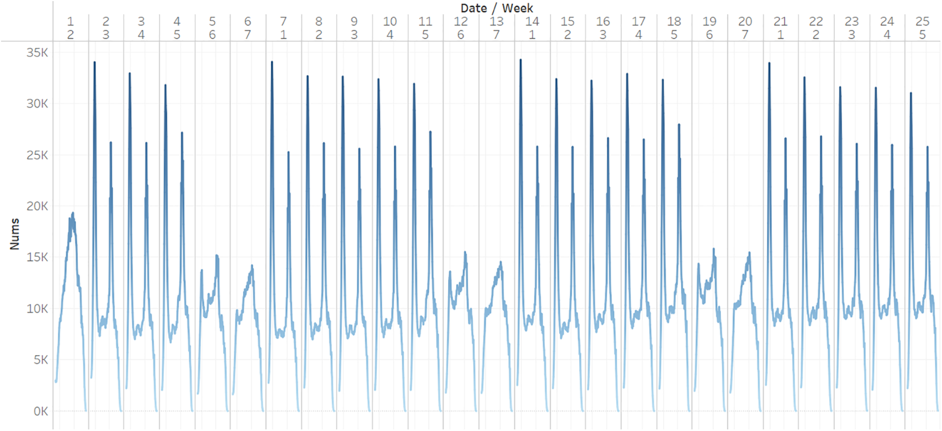
Figure 1: The total number of incoming passengers in Hangzhou subway

To investigate the relationship between ridership and legal working hours, Fig. 2 displays the daily number of passengers at all stations. The working days in January, as defined by legal regulations, are indicated by warm colors, while the weekends are represented by cold colors (specifically, the 5th, 6th, 12th, 13th, 19th, and 20th days).

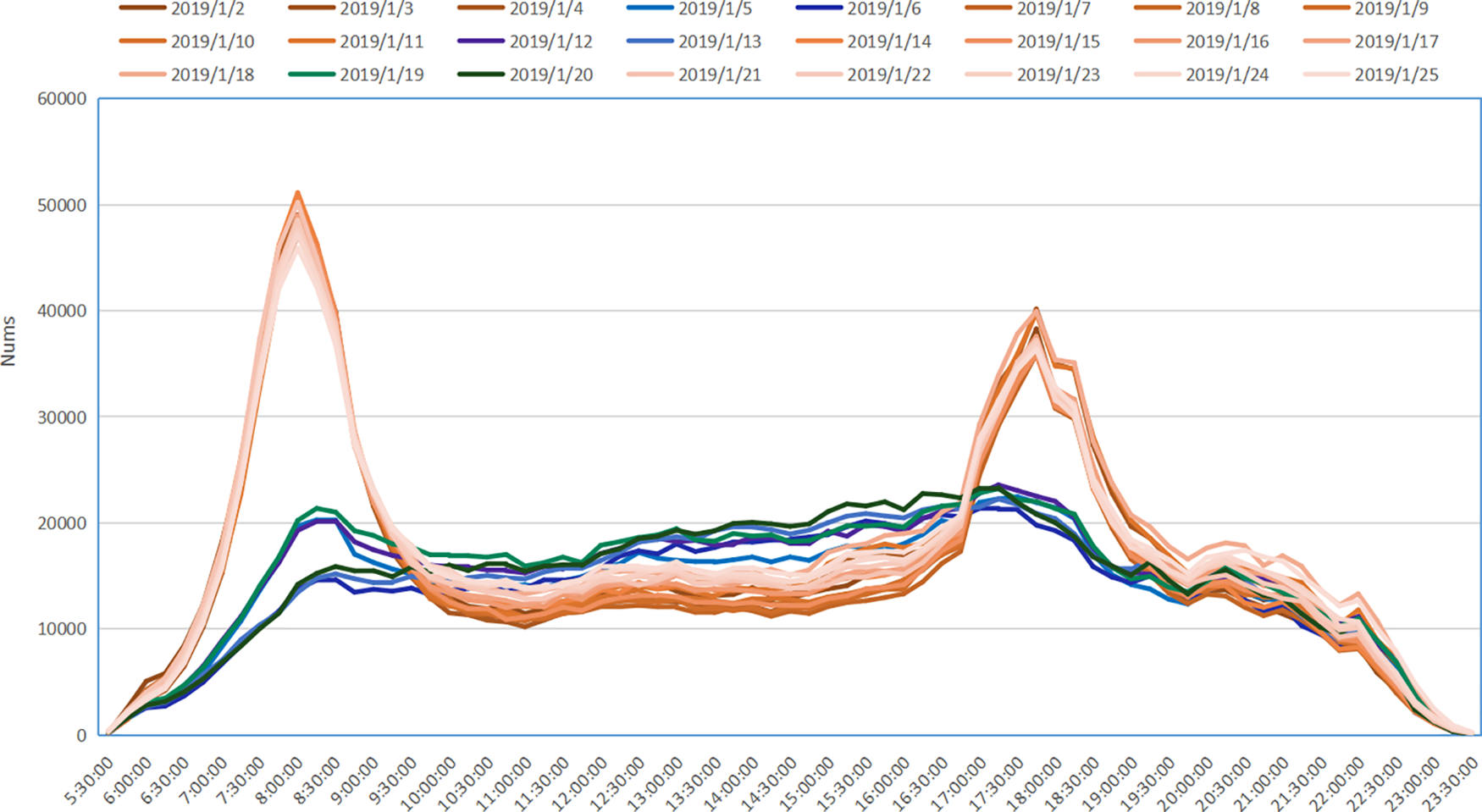
Figure 2: The total number of Hangzhou subway stops in daily and time

A clear trend can be observed in the weekday passenger flow, with two distinct peak periods from 7:00 to 9:00 am and 17:00 to 19:00 pm. During these rush hours, the number of passengers significantly exceeds the daily average, and the morning peak can even reach 2.5 times the non-rush hour count. In contrast, the number of passengers on weekends drastically decreases, and there are no distinct rush hour patterns as seen on weekdays. Therefore, it can be determined that peak periods also play a crucial role in influencing passenger flow. In this study, the time frames of 7:00–9:00 and 17:00–19:00 are designated as rush hours for commuting.

Based on the analysis of the time characteristics, the original AFC records are processed following the aforementioned feature extraction methods. Xianghu Station, which is the 0 station of Line 1, is chosen as the test station. The data from this station is divided into a 20% test dataset, and the remaining 80% is used for training the model.

3  Methodologies

3.1 Characteristic Engineering

3.1.1 Variational Modal Decomposition (VMD)

The VMD algorithm is employed for decomposing arbitrary data signals to extract their underlying intrinsic information. VMD is a non-recursive adaptive modal variational process. It formulates the variational problem as solving a constraint equation on the smallest possible finite broadband sum of modal components around an optimal central frequency [1]. The constructed constraint model is the following:

{min{vk},{wk}{∑k=1K‖∂t[(δ(t)+jπt)∗vk(t)]e−jwkt‖2}s.t.∑kvk(t)=f(t)(1)

In the above model, {vk} = {v1, v2, v3, ..., vk} are the intrinsic modal functions (IMFs). {wK} = {w1, w2, w3, ..., wk} are the center frequency of corresponding IMF components.

The algorithm aims to discover a set of IMFs and their respective corresponding central frequencies from the raw data signal according to a certain frequency range, achieving an efficient decomposition of specific components in a given signal. The effectively separated IMFs are the optimal solution of the constraints. To solve the model, the Lagrange multiplier γ and the second-order penalty factor α are introduced to transform the constraint problem into an unconstrained problem, namely:

L({vk},{wk},γ)=α∑k=1K‖∂t[(δ(t)+jπt)∗vk(t)]e−jwk(t)‖2+‖f(t)−∑k=1Kvk(t)‖2+⟨γ(t),f(t)−∑k=1Kvk(t)⟩(2)

The variational model is used to iteratively obtain the optimal model solution, making the model more robust to the sampling noise. The calculation process is performed as follows:

1.    Initialize {vk } , {wk }, γ, n = 0.

2.    Enter the cycle process and constantly iterating by n = n + 1.

3.    According to the modal component formula (3), constantly updated.

vk,n+1(w)=f^(w)−∑i≠kv^i(w)+γ^(w)/21+2α(w−wk)2(3)

where, the Fourier transform f^(w), v^k,n+1(w), γ^(w) are corresponding to f(w), vk,n+1(w), γ(w).

4.    According to the central frequency formula (4), constantly updated.

wk,n+1=∫0∞w|vk,n+1(w)|2dw∫0∞|vk,n+1(w)|2dw(4)

5.    According to the Lagrange multiplier formula (5), constantly updated.

γ^n+1(w)=γ^n(w)+γ(f^(w)−∑k=1Kv^k,n+1(w))(5)

6.    Steps 2 to 5 are repeated until a satisfactory minimum broadband sum and K modal components found.

∑k=1K‖v^k,n+1−v^k,n‖2‖v^k,n‖2<ε(6)

The passenger flow sequence is considered as the information flow of traffic signals across various dimensions. In short-term passenger flow prediction, the VMD algorithm is utilized to decompose the passenger flow information into K modal components with different time dimensions centered around the central frequency. These time dimensions include monthly mode, weekly mode, daily mode, hourly mode, and more. This time granularity is chosen for 15 min, the K is 7, to obtain the final IMFs, as shown in Fig. 3. To avoid modal crossing, K-means is used for modal screening, and finally retained the modal data of the three dimensions.

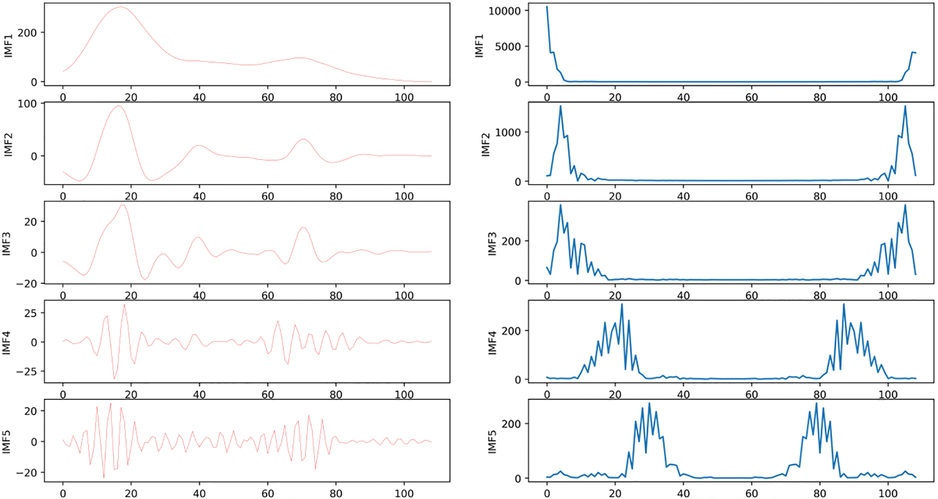
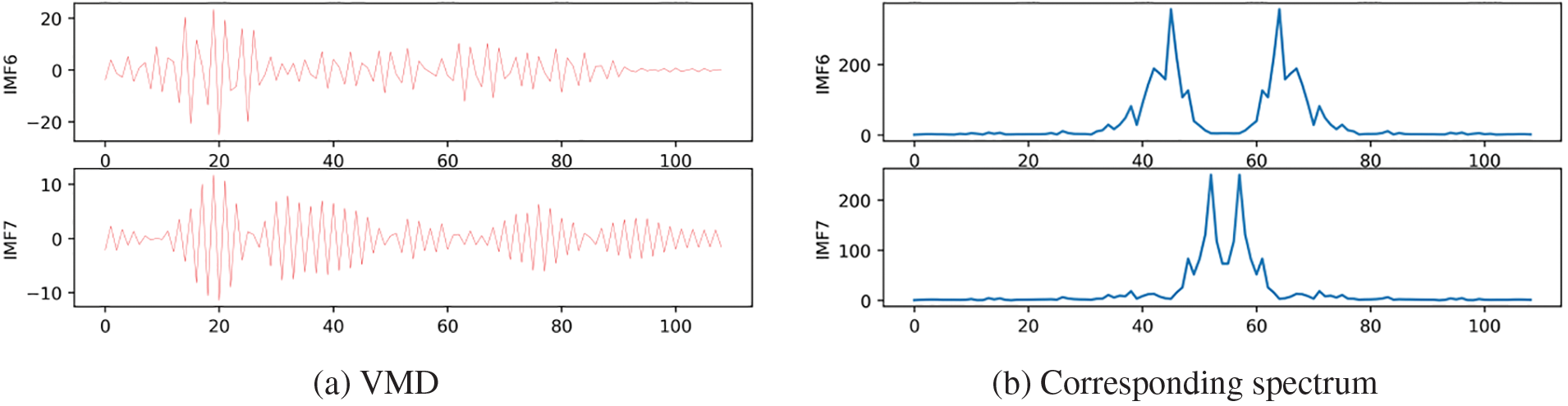
Figure 3: The decomposition results

3.1.2 Objective Environmental Characteristics

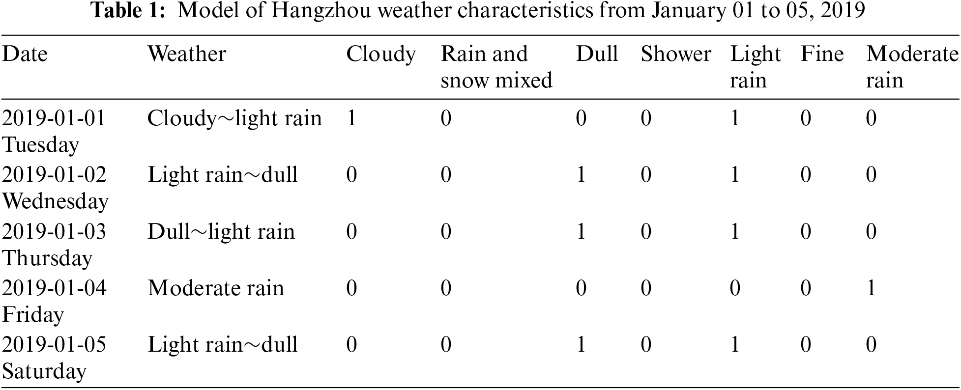
From Figs. 1 and 2, it is evident that traffic flow is associated with the presence of weekends and commuting peaks. Scholars have also verified that weather conditions significantly impact commuting choices. Extreme weather conditions like heavy rain and haze tend to reduce the likelihood of people attending work or other activities, whereas clear weather tends to encourage more travel and movement [32]. Scholars have conducted studies to verify the influence of various weather factors on passenger flow. They have used Pearson’s correlation coefficient to assess the impact of temperature, humidity, visibility, and cloud volume on passenger flow [10]. Additionally, researchers have introduced 11 external factors, including temperature, climate, and Air Quality Index (AQI), to explore the correlation between weather and subway traffic flow [24,33].

This paper utilizes crawler technology to gather environmental data for Hangzhou in January 2019. The collected data includes various parameters such as maximum temperature, minimum temperature, weather conditions, wind direction, and air quality. At the same time, text data (such as cloudy, light rain) is transformed into numerical data types that the model can identify. Table 1 shows the weather characteristic word pouch cases.

3.1.3 K-Nearest Neighbor (KNN)

The fundamental principle of the KNN algorithm is that “similar objects tend to cluster together”. In other words, objects with similar characteristics are closer to each other. In a classification task, the KNN algorithm utilizes this principle by analyzing a training dataset, where each sample is labeled. To predict the category of a new instance sample, it finds the similarity between the new instance and the K nearest samples based on a similarity metric. The algorithm then assigns the prediction category of the new instance based on the labels of these nearest neighbors. Moreover, the proximity of samples in the feature space reflects their degree of similarity. Thus, KNN is capable of clustering samples and identifying those with similar characteristics.

In subway traffic prediction, besides considering the historical records of a specific station (e.g., the previous traffic values) and weather conditions (such as current climate information), it is also beneficial to incorporate the historical data from other stations that exhibit similar trends. By considering the overall spatial layout of the entire traffic network, this approach can provide valuable insights and complement the feature information specific to the target station. To establish the relationship between the historical characteristics of a target station and other stations, and to gather valuable information for predicting the passenger flow, this research employs a methodology that explores the most similar K stations exhibiting similar trends within a specified time range. The historical data from these similar stations is then utilized as supplementary information for training the prediction model.

Setting K = 3, as depicted in Fig. 4, the historical data of the three most similar stations at 8:45 on January 9th is shown. An observation from the figure reveals that these most similar stations exhibit traffic flow trends that are relatively consistent with the target station. This valuable information can serve as a reference for training the prediction model.

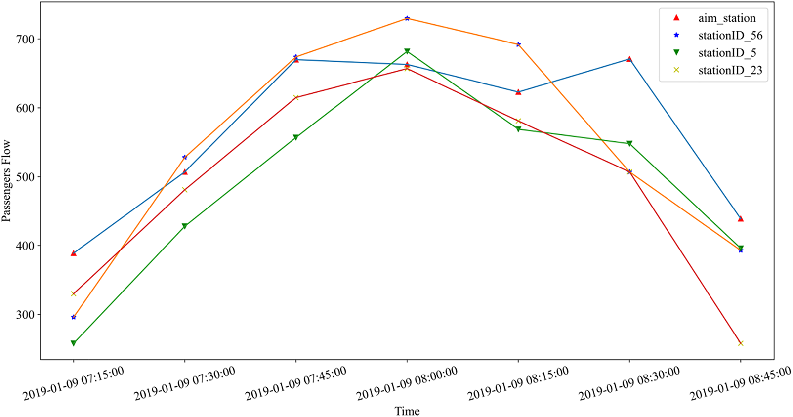
Figure 4: The similar station’s passengers flow of 0 station

3.2 Model Theory

3.2.1 Long and Short-Term Memory (LSTM)

While inheriting the strengths of the recurrent neural network (RNN) model, LSTM overcomes its memory limitations in a relatively short time. It also possesses the capability to selectively retain information based on the current situation, enabling it to be applicable to training sets with intervals or delays. When dealing with large datasets, the effectiveness of LSTM in handling time-related characteristics becomes especially pronounced. LSTM excels in capturing both linear and non-linear time features, allowing it to outperform conventional linear methods. Its ability to capture time series-dependent features has led to widespread utilization and remarkable success in various fields today.

The structure of LSTM is shown in Fig. 5. It is not difficult to find that LSTM updates the hidden state h(t) and cell state c(t) at the current moment by the output values h(t−1), c(t−1) at the previous time. In Fig. 5, Sigmoid and Tanh activation functions are represented as σ and τ, respectively. Notably, the dashed line represents that the LSTM cell cycle update such that the cell state (c(t)) and hidden state (h(t)) as current state input, calculating the next moment cell (c(t+1)) and hidden state (h(t+1)).

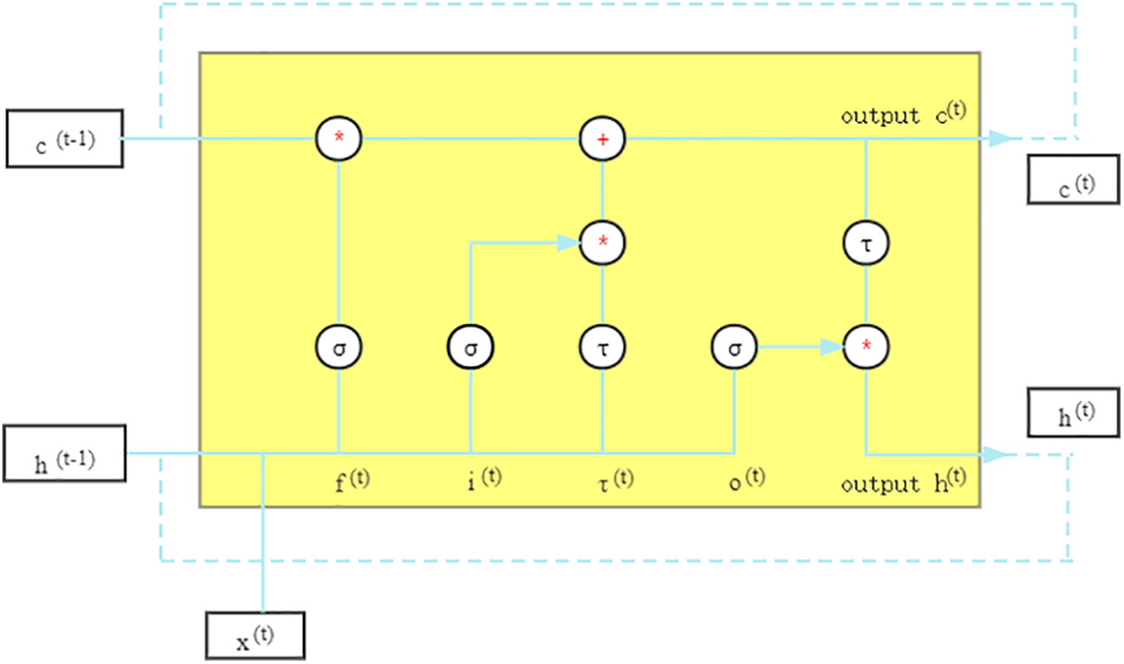
Figure 5: Structure illustration of LSTM cells

The LSTM unit calculation process is as follows:

Step1: The forgetting gate and the input gate consume the information from the input units (h(t−1) and x), to identify which information comes from the output of the previous state, and to determine which information need to be forgotten.

i(t)=σ(Wix⋅x(t)+Wih⋅h(t−1)+bi)(7)

f(t)=σ(Wfx⋅x(t)+Wfh⋅h(t−1)+bf)(8)

o(t)=σ(Wox⋅x(t)+Woh⋅h(t−1)+bo)(9)

where, σ represents the Sigmoid activation function, Wix and Wih indicate the weight of the input gate, and bi indicates the bias of the input gate. Similarly, Wjx, Wjh and bf represent the weights and bias of the forgetting gate, and Wox, Woh and bo indicate the weights and bias of the output gate.

Step2: Each LSTM unit also contains a separate nonlinear Tanh activation function that is called c~ neural network that determines which part of the input information will be stored in the unit state.

c~(t)=tanh⁡(Wc~x⋅x(t)+Wc~h⋅h(t−1)+bc~)(10)

where, Wc~x, Wc~h, bc~ and represent weights and biases of the neural network.

Step3: Formulas (11) and (12) update the current cell state c(t) and hidden state h(t), respectively.

c(t)=f(t)∗c(t−1)+i(t)∗c~(t)(11)

h(t)=tanh⁡(c(t))∗o(t)(12)

Therefore, deep learning can effectively utilize the inherent strengths of LSTM in handling time series data, thus enabling the extraction of valuable time series features.

3.2.2 Convolutional Neural Network (CNN)

CNN is capable of efficiently extracting feature information using convolution layers and pooling layers. Through the convolution process, neurons in the convolutional kernel move based on specified strides, allowing them to capture local information from the data tensor. By integrating this local information, CNN can derive global spatial features at a higher level. In the case of passenger flow data between similar stations, it contains layout information about urban stations, which encompasses their spatial characteristics to some extent. By utilizing CNN, valuable spatial features can be extracted for predicting passenger flow. Specifically, the convolutional layer distributes global information linearly by extracting it from local data tensors.

CNN incorporates two fundamental ideas: local receptive field and weight sharing. The local receptive field is embodied in the convolutional kernel, where only relevant information from a specific local region is extracted at each step. This allows for stability in terms of displacement, nonlinearity, and deformation. Weight sharing, on the other hand, enables the sharing of parameters among different neurons. By updating the weights just once, all calculations for each stride can be completed. Consequently, the number of parameters is significantly reduced. Moreover, local linear calculations lead to global nonlinear transformations.

Given these characteristics, CNN is well-suited for extracting multidimensional feature information, which can be employed to capture additional spatial features.

4  Hybrid Model of Short-Term Passenger Flow Prediction

4.1 Building Prediction Model

Rail transit passenger flow is a representative example of time series data, where the flow sequence is influenced by historical flows, current objective environmental factors, and the layout of the transit system as a whole. In light of this, this research paper sequentially applies VMD to decompose the passenger flow data, LSTM to model the temporal dependencies in the data, and CNN to extract spatial features. As a result, a hybrid deep learning model called VMD-CLSTM is proposed for short-term passenger flow prediction in rail transit.

The network structure, as depicted in Fig. 6, consists of two distinct stages:

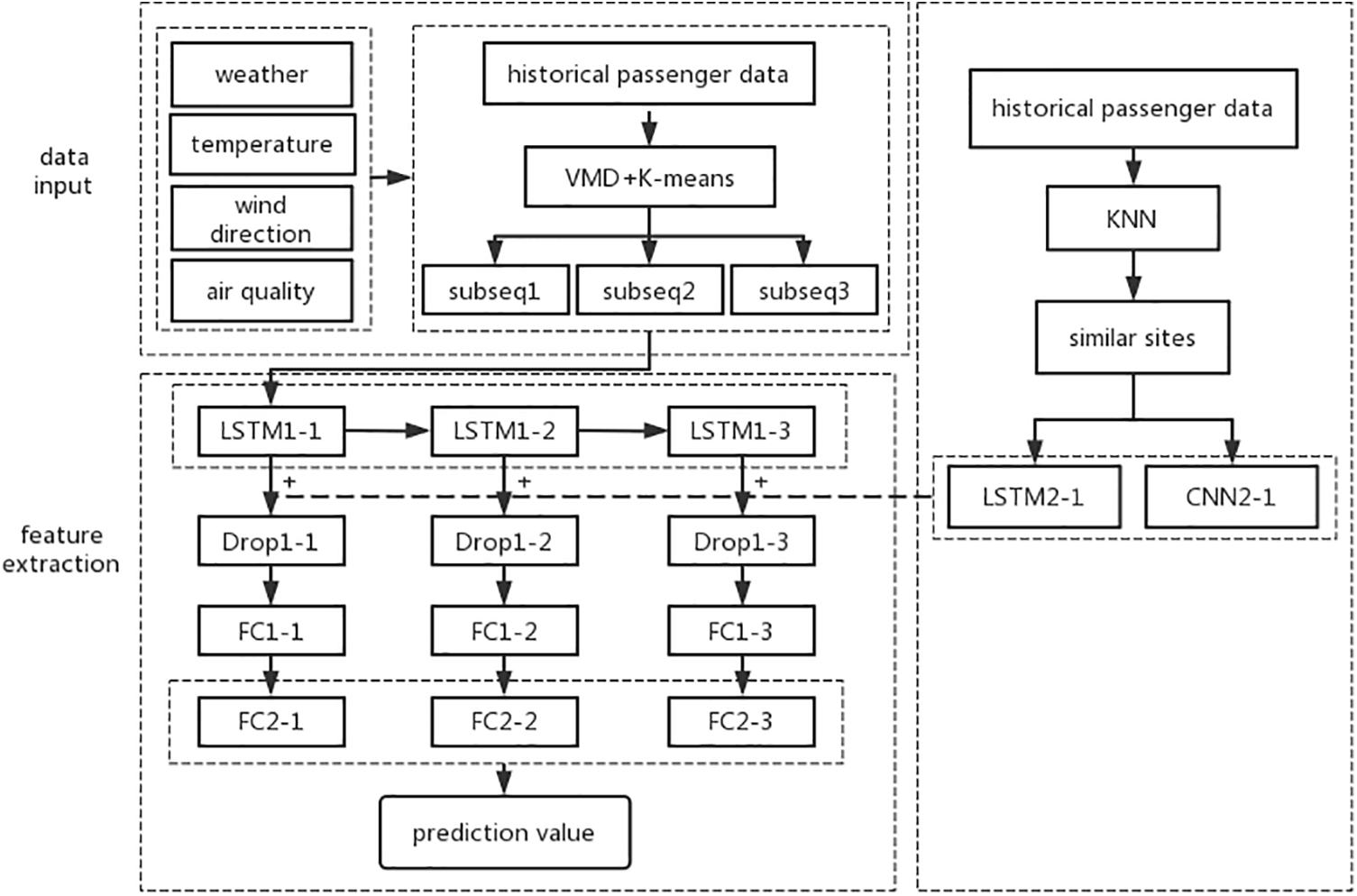
Figure 6: The structure diagram of the VMD-CLSTM network

Stage 1: Data input and feature engineering. The data used for training the model is divided into three components. The first component comprises the original passenger flow sequence after applying the VMD technique. The second component consists of objective environmental characteristics factors. The third component is derived from similar passenger flow patterns identified through the KNN algorithm. In this stage, the preprocessed passenger flow data is decomposed using variational mode decomposition, retaining three-dimensional sequences. The external objective environmental data is then added to the decomposed modal components. Lastly, the KNN algorithm is utilized to identify reference sites with passenger flow trends similar to the target site over a short duration, acting as additional input features.

Stage 2: Feature extraction and passenger flow prediction. In this stage, the data obtained in Stage 1 are utilized in the network for the extraction of features and prediction of passenger flow. The main sequences consist of higher-dimensional sequences obtained by combining the data after applying VMD with the objective environmental data. These sequences are inputted into the LSTM1 layers, where regular information related to temporal features is extracted. Since the similar spatial supplementary features encompass both temporal and spatial characteristics, this subset of data is fed into the LSTM2 and CNN2 layers to extract relevant features. Subsequently, these features are integrated into the main sequences. This integration results in the main data sequences containing more specific temporal and spatial features, enriching the subsequent information processing. To prevent overfitting of the model during training, Drop layers are incorporated to randomly reduce the number of neurons. The FC1 (FC denotes the fully connected layer in deep learning representing the backward propagation model) and FC2 layers serve as information processing networks, transforming concrete features into abstract features. These layers utilize information from the last n time steps to reason about the passenger flow for the next time step, enhancing prediction accuracy through reverse derivation mechanism. The training labels encompass the historical passenger counts, while the objective of the prediction is the passenger flow for the next time step.

4.2 Residual Network (ResNet)

Fig. 7 illustrates the residual module, which comprises multiple network layers (e.g., CNN or other arbitrary network layers). The output F(X) is obtained by feeding the data X through the activation function (e.g., ReLU) of the multi-layer network. Simultaneously, the original input X is passed through multiple network layers without any changes and then added directly to F(X) as a residual connection. This combined result is then passed through the next activation function in the subsequent stage for further computation. Essentially, the output result of the residual network, F(X) + X, not only contains the processed information from the intermediate network layers but also retains the original data, which compensates for any information loss that may occur during the computation in the intermediate layers. This technique addresses the problem of information loss in the intermediate layers and overcomes the issue of gradient vanishing or exploding due to increased network depth.

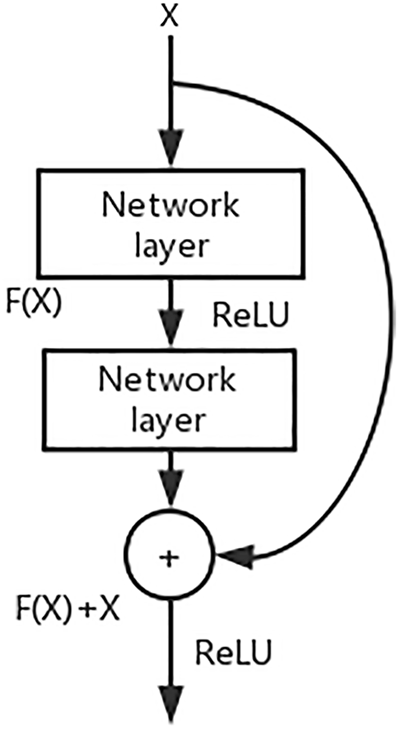
Figure 7: Residual structure

4.3 Model Optimization Is Based on the Residual Network

The residual learning approach has been applied to short-term passenger flow prediction in rail transit research. The model is divided into two levels: the first-order prediction model and the second-order prediction model, as shown in Fig. 8.

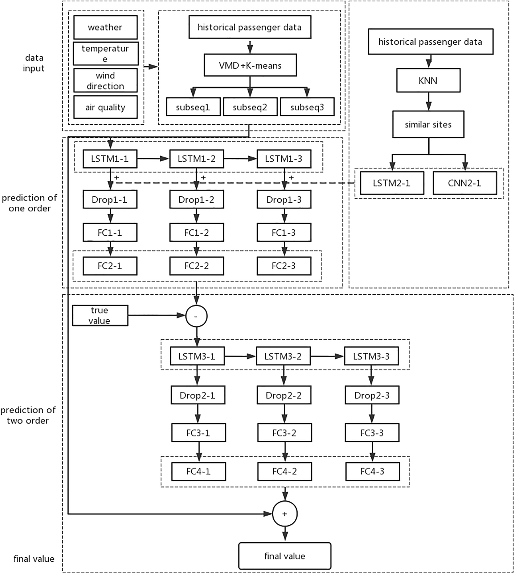
Figure 8: The structure of hybird model VMD-CLSTM with two orders

The first-order prediction model focuses on feature extraction and predicting the number of passengers, as described in Section 4.1. The prediction result of the first-order model is the number of passenger flows at the next moment.

The second-order prediction model focuses on improving the accuracy of the overall model. It is designed to further enhance the accuracy of the predictions. The input for the second-order model is the same as the first-order model, with the only difference being the predicted targets. In the first-order model, the prediction labels are the number of passengers at the next time step, while in the second-order model, the prediction labels represent the deviation between the first-order prediction result and the real passenger flow data. The objective of the second-order model is to correct the predictions made by the first-order model.

5  Example Analysis

5.1 Basic Setting

The research utilizes the Intel Core i7 CPU platform along with the third-party libraries scikit-learn, vmdpy, and TensorFlow within the Jupyter environment based on Python 3.8. The hyperparameters of the VMD-CLSTM model are configured as follows: the model utilizes 128 LSTM units with a time step of 4. Additionally, the model employs a CNN with 32 convolution kernels of size 2 × 2. The fully connected layers consist of 128 and 32 neurons, respectively. The activation function used throughout the entire network is ReLU. The loss function used is MSE, and the Adam optimizer is utilized. To mitigate over-fitting, early stop monitoring is implemented during the training phase, with a min_delta value of 0.01 and a tolerance of 5.

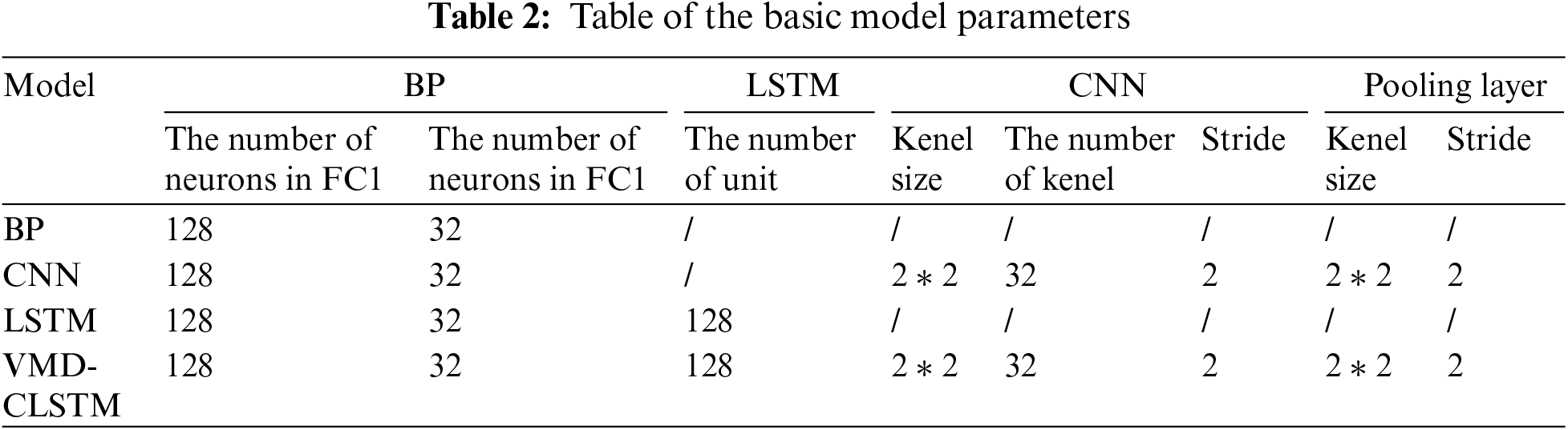
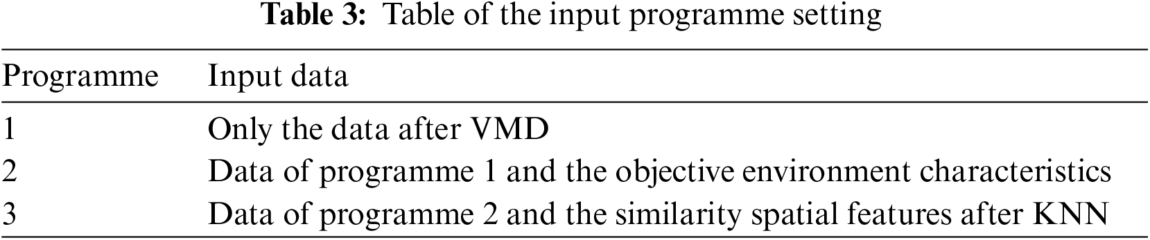
To validate the effectiveness of the supplementary features and the hybrid model, reference models including the Backward Propagation Network (BP), CNN, and LSTM are employed. Table 2 provides the parameters for these reference models. Additionally, Table 3 illustrates three feature input schemes used in the study.

This paper utilizes several performance metrics to evaluate the prediction models: mean absolute error (MAE), root mean square error (RMSE), mean square error (MSE), and determination coefficient (R2). The R2 is a measure that ranges from 0 to 1. A value closer to 1 indicates a better fitting effect. In particular, a value greater than 0.8 suggests a highly accurate fit. On the other hand, MAE, RMSE, and MSE are used as error metrics. Larger values of MAE, RMSE, and MSE indicate poorer prediction performance, implying a larger deviation between the predicted values and the actual values.

5.2 Comparative Analysis with Basic Models

Table 4 presents the evaluation metrics for VMD-CLSTM and the basic models. In comparison to the BP, CNN, and LSTM models, the VMD-CLSTM model demonstrates lower values for MSE, RMSE, and MAE, calculated at 1413.14, 37.59, and 25.87, respectively.

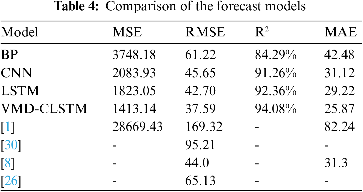
Additionally, Fig. 9 illustrates that VMD-CLSTM achieves the best performance with an R2 value of 94.08%, surpassing the BP, CNN, and LSTM models by 9.79%, 2.82%, and 1.72%, respectively. This highlights the advantage of the VMD-CLSTM model, which combines the strengths of LSTM and CNN.

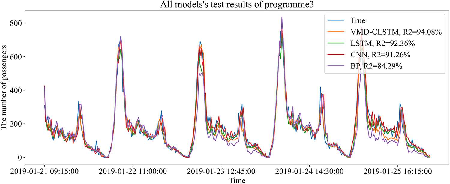
Figure 9: Comparison of the forecast results of VMD-CLSTM and base models

Table 4 not only presents the evaluation results of the VMD-CLSTM model, but also includes the performance of existing models on 15-min granularity prediction. It is observed that the existing research [1,30,8], and reference [26] achieved RMSE values of 169.32, 95.21, 65.13, and 44.0, respectively, which are higher than the RMSE value of 37.54 obtained by the hybrid model VMD-CLSTM. Furthermore, the MSE value of 28669.43 in [1] is significantly larger than the VMD-CLSTM value of 1413.14. Additionally, the MAE value of 25.87 in VMD-CLSTM is lower than the 31.3 reported in reference [8]. The comprehensive analysis indicates that the VMD-CLSTM model surpasses the existing models in terms of prediction accuracy. In conclusion, the VMD-CLSTM model is suitable for short-term passenger flow prediction in rail transit applications and achieves higher accuracy compared to both the basic models and existing models.

5.3 Comparative Analysis of the Ablation Experiments

To examine the importance of objective environment factors and supplementary similarity features, the three different feature input schemes are tested using the control variable method. A total of 12 experiments are conducted, and the prediction results are presented in Table 5 and Fig. 10. It is evident from the results that the VMD-CLSTM model consistently achieves the smallest values for MSE, RMSE, and MAE across all three feature input schemes. Furthermore, the VMD-CLSTM model achieves the highest R2 values of 90.25%, 92.16%, and 94.08% respectively for each scheme. These findings highlight the superiority of the VMD-CLSTM model over the BP, CNN, and LSTM models in passenger flow prediction for rail transit. This confirms that the VMD-CLSTM model exhibits higher accuracy compared to the other basic models.

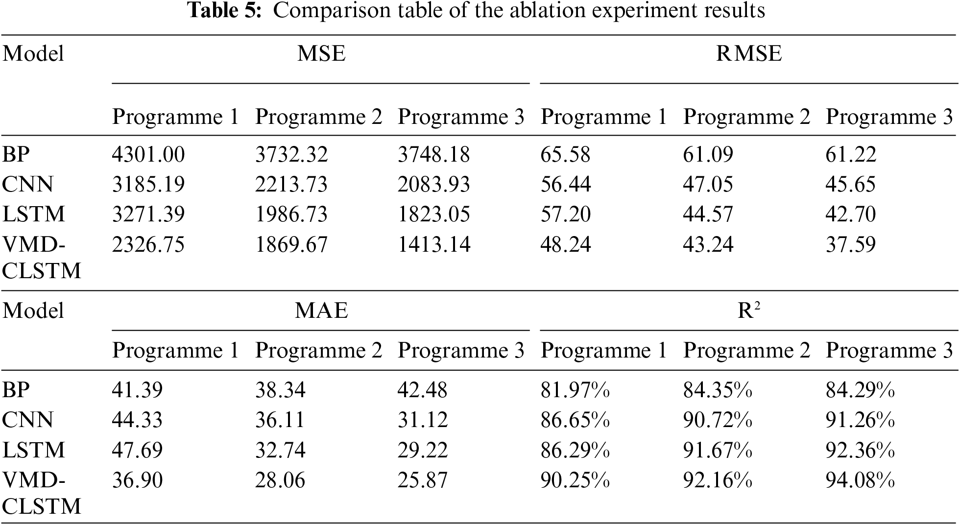
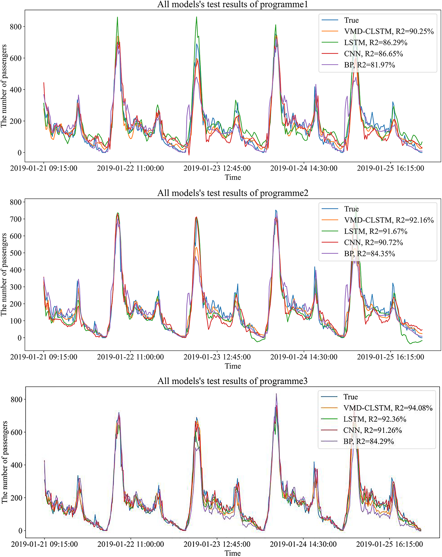
Figure 10: Comparison of each mode’s effect under the three schemes

In the comparison between Programme 1 and Programme 2, it is observed that the MSE, RMSE, and MAE indices of each model in Programme 2 are lower than those in Programme 1. For example, the RMSE value of VMD-CLSTM is 43.24 in Programme 2, which is smaller than the RMSE value of 48.24 in Programme 1. This demonstrates that the prediction results in Programme 2 are better than those in Programme 1. These findings indicate that objective environment features can enhance the accuracy of prediction, affirming the positive impact of considering objective environment factors in feature engineering.

Comparing Programme 3 to Programme 2, it is observed that all four models achieve improved prediction results in Programme 3. For instance, the VMD-CLSTM model achieves the highest R2 value of 94.08% in Programme 3, which is 3.83% and 1.92% higher than that in Programme 1 and Programme 2, respectively. Additionally, the three basic models (BP, CNN, and LSTM) in Programme 2 do not match the accuracy attained in Programme 3. The comparison between Programme 2 and Programme 3 demonstrates that incorporating similar stations’ supplementary characteristics improves the accuracy of short-term passenger flow prediction and enhances the model’s robustness.

In summary, mining objective environment features and incorporating similar stations’ supplementary features aligns with the passenger flow sequence pattern, enabling the model to achieve better training results. This highlights that the model trained using both objective environment features and similar stations’ supplementary features yields the best prediction performance.

5.4 Comparative Analysis of the Residual Networks

To enhance the prediction accuracy of short-term passenger flow in rail transit, the concept of residuals is introduced into the prediction model. The effectiveness of the residual network is then verified. The first and second-order prediction performance of the four models under the three aforementioned schemes is presented in Figs. 11 to 13.

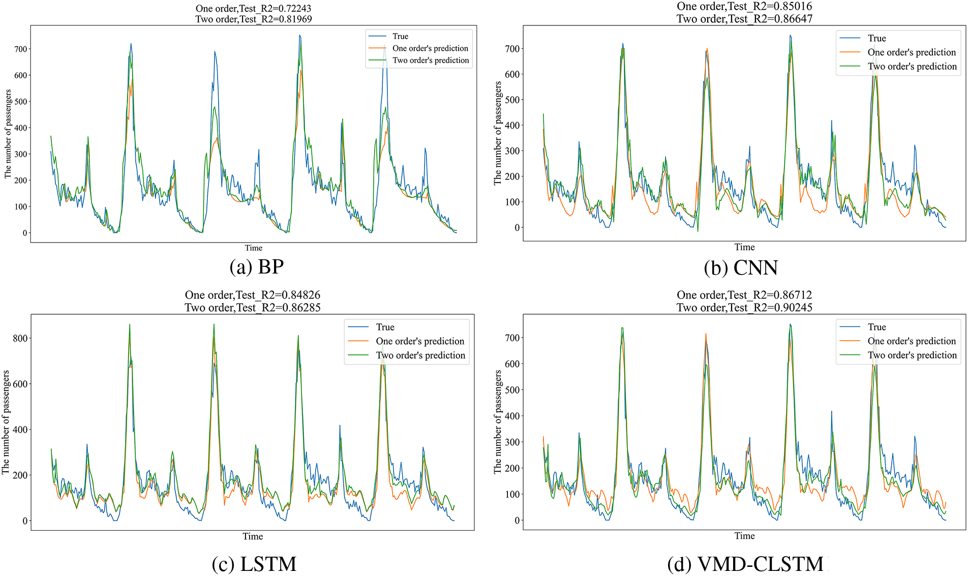
Figure 11: Comparison of the first and second order results of the four models in Programme 1

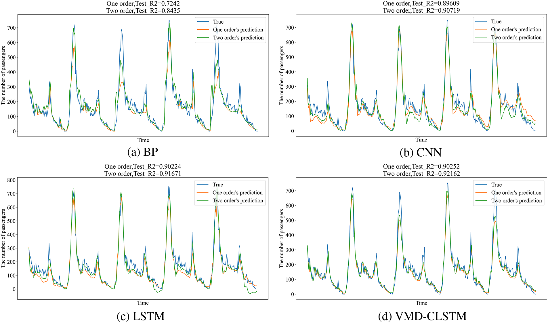
Figure 12: Comparison of the first and second order results of the four models in Programme 2

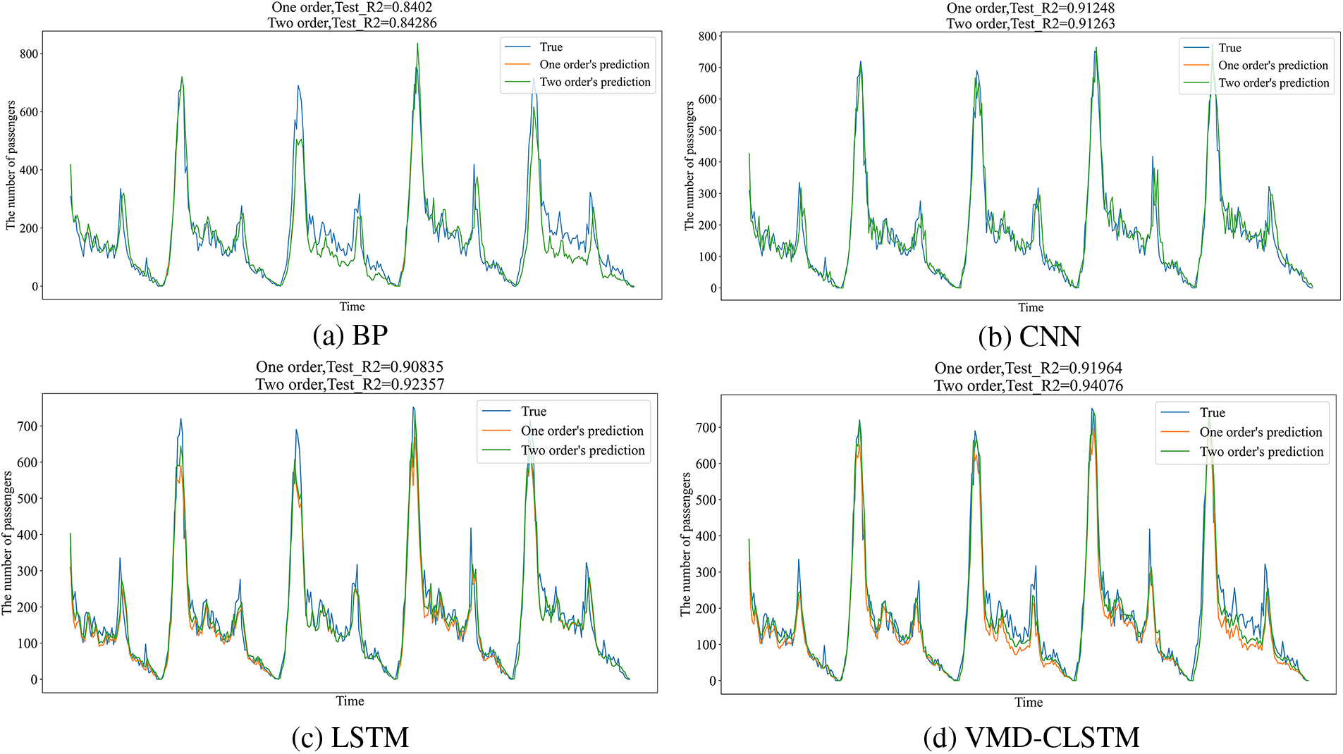
Figure 13: Comparison of the first and second order results of the four models in Programme 3

Observing the figures, it is evident that the second-order R2 values of each model are higher than the corresponding first-order values. Furthermore, the BP network exhibits the most significant improvement under Programme 2, with a difference in R2 of 11.93%. These results demonstrate the capability of the residual network to enhance the accuracy of the model.

6  Conclusion

Based on the principles and characteristics of deep learning models, the VMD-CLSTM hybrid model was proposed for short-term passenger flow prediction in rail transit. Through reference experiments and different programs, the following conclusions were drawn:

(1) The VMD-CLSTM hybrid model, combining CNN and LSTM, demonstrated higher reliability compared to the BP, CNN, and LSTM basic models for short-term passenger flow prediction.

(2) Ablation experiments with three different programs confirmed that incorporating objective environment factors and supplementary spatial features improved the model's accuracy and robustness.

(3) Comparing first-order and second-order prediction results from 12 sets of experiments revealed that all models achieved higher prediction accuracy in the second order, affirming the reliability of the residual network in short-term passenger flow prediction.

However, it is important to note that there are several factors influencing rail transit passenger flow that were not considered in this research, such as holidays and special events. In the future, expanding the dataset to include a larger time span and collecting passenger flow data during holidays and special activities could further enhance the model's accuracy. Additionally, the time granularity of the data could be optimized, and the model could be developed to predict passenger flow for different time granularities.

Acknowledgement: We also extend special thanks to the editor/reviewers for their valuable comments in improving the quality of this paper.

Funding Statement: This work was supported by the Major Projects of the National Social Science Fund in China (21&ZD127).

Author Contributions: The authors confirm contribution to the paper as follows: study conception and design: Song Yinghua, Zhang Wei; data collection: Zhang Wei; analysis and interpretation of results: Zhang Wei, Lyu Hairong; draft manuscript preparation: Lyu Hairong. All authors reviewed the results and approved the final version of the manuscript.

Availability of Data and Materials: This study will utilize the Automatic Fare Collection (AFC) card swipe records from the Hangzhou subway system as the training data for this experiment. The data is sourced from the inaugural Global Urban Computing AI Challenge jointly organized by Hangzhou Municipal Public Security Bureau and Alibaba Cloud Intelligence. The competition provided entry and exit records for all stations on three subway lines in Hangzhou, covering the time period from January 01, 2019 to January 25, 2019. The data is divided into daily documents, consisting of a total of 25 files.

Conflicts of Interest: The authors declare that they have no conflicts of interest to report regarding the present study.

References

1. J. Wu, Y. Q. He, N. Zhang and H. F. Wu, “Forecast of short-term passenger flow of urban rail transit based on VMDGRU,” Urban Rapid Rail Transit, vol. 35, no. 1, pp. 79–86, 2022. [Google Scholar]

2. L. M. Pan, “Research on forecasting and warning of short-term passenger flow in metro,” M.S. Thesis, Capital University of Economics and Business, China, 2011. [Google Scholar]

3. P. C. Meng, X. Y. Li and H. F. Jia, “Short-time rail transit passenger flow real-time prediction based on moving average,” Journal of Jilin University (Engineering and Technology Edition), vol. 48, no. 2, pp. 448–453, 2018. [Google Scholar]

4. J. Xiong, W. Guan and Y. X. Sun, “Metro transfer passenger forecasting based on Kalman Filter,” Journal of Beijing Jiaotong University, vol. 37, no. 3, pp. 112–116, 2013. [Google Scholar]

5. R. Leng, “Research on the flow forecast of subway in and out station based on SAE-LSTM,” in Scientific and Technological Papers of the 15th China Intelligent Transportation Annual Conf., Shenzhen, China, pp. 199–209, 2020. [Google Scholar]

6. H. Y. Li, Y. T. Wang, X. Y. Xu, L. Q. Qin and H. Y. Zhang, “Short-term passenger flow prediction under passenger flow control using a dynamic radial basis function network,” Applied Soft Computing, vol. 83, pp. 105620, 2019. [Google Scholar]

7. Q. Z. Yang, H. B. Zhang and J. Li, “Analysis of passenger flow prediction and organizational countermeasures of Weijianian,” Scientific and Technological Innovation, vol. 22, pp. 152–155, 2022. [Google Scholar]

8. Y. Z. Xu, L. Peng and H. Lin, “Short-term passenger flow prediction in Shanghai subway system based on stacked autoencoder,” Computer Engineering & Science, vol. 40, no. 7, pp. 1275–1280, 2018. [Google Scholar]

9. Y. K. Wu, H. C. Tan, L. Q. Qin, B. Ran and Z. X. Jiang, “A hybrid deep learning based traffic flow prediction method and its understanding,” Transportation Research Part C: Emerging Technologies, vol. 90, no. 2554, pp. 166–180, 2018. [Google Scholar]

10. H. Z. Zhang, Z. K. Gao and J. Q. Li, “Short-term passenger flow forecasting of urban rail transit based on recurrent neural network,” Journal of Jilin University (Engineering and Technology Edition), vol. 53, no. 2, pp. 430–438, 2022. [Google Scholar]

11. Y. Hu and H. Liu, “Prediction of passenger flow on the highway based on the least square support vector machine,” Transport, vol. 26, no. 2, pp. 197–203, 2011. [Google Scholar]

12. J. Roos, G. Gavin and S. Bonnevay, “A dynamic bayesian network approach to forecast short-term urban rail passenger flows with incomplete data,” Transportation Research Procedia, vol. 26, no. 2, pp. 53–61, 2017. [Google Scholar]

13. S. Yu, C. Shang, Y. Yu, S. Zhang and W. Yu, “Prediction of bus passenger trip flow based on artificial neural network,” Advances in Mechanical Engineering, vol. 8, no. 10, pp. 211–234, 2016. [Google Scholar]

14. N. G. Polson and V. O. Sokolov, “Deep learning for short-term traffic flow prediction,” Transportation Research Part C: Emerging Technologies, vol. 79, no. 2, pp. 1–17, 2017. [Google Scholar]

15. Y. Wei and M. C. Chen, “Forecasting the short-term metro passenger flow with empirical mode decomposition and neural networks,” Transportation Research Part C: Emerging Technologies, vol. 21, no. 1, pp. 148–162, 2012. [Google Scholar]

16. L. L. Gong and X. H. Ling, “Experimental design of short-term bus passenger flow forecasting based on LSTM,” Modern Electronics Technique, vol. 44, no. 22, pp. 97–100, 2021. [Google Scholar]

17. X. Ma, Z. Dai, Z. He, J. Ma, Y. Wang et al., “Learning traffic as images: A deep convolutional neural network for large-scale transportation network speed prediction,” Sensors, vol. 17, no. 4, pp. 818, 2017. [Google Scholar] [PubMed]

18. X. Fu, Y. F. Zuo, J. J. Wu, Y. Yuan and S. Wang, “Short-term prediction of metro passenger flow with multi-source data: A neural network model fusing spatial and temporal features,” Tunnelling and Underground Space Technology, vol. 124, no. 2, pp. 104486, 2022. [Google Scholar]

19. Y. Bai, Z. Z. Sun, B. Zeng, J. Deng and C. Li, “A multi-pattern deep fusion model for short-term bus passenger flow forecasting,” Applied Soft Computing, vol. 58, no. 1, pp. 669–680, 2017. [Google Scholar]

20. G. Xue, S. F. Liu, L. Ren, Y. C. Ma and D. Q. Gong, “Forecasting the subway passenger flow under event occurrences with multivariate disturbances,” Expert Systems with Applications, vol. 188, no. 4, pp. 116057, 2022. [Google Scholar]

21. X. R. Zhang, C. Liu and Z. Chen, “Short-term passenger flow prediction of airport subway based on spatio-temporal graph convolutional,” Computer Engineering and Applications, vol. 59, no. 8, pp. 322–330, 2023. [Google Scholar]

22. X. Q. Wang, X. Y. Xu and Y. K. Wu, “Short term passenger flow forecasting of urban rail transit based on hybrid deep learning model,” Journal of Railway Science and Engineering, vol. 19, no. 12, pp. 1–11, 2022. [Google Scholar]

23. Y. He and D. Li, “Real-time subway ridership detection based on YOLOv5 and DeepSort,” Electronic Test, vol. 36, no. 2, pp. 46–48, 2022. [Google Scholar]

24. T. X. Peng, Y. Han, C. Wang and Z. H. Zhang, “Hybrid deep-learning model for short-term metro passenger flow Prediction,” Computer Engineering, vol. 48, no. 5, pp. 297–305, 2022. [Google Scholar]

25. W. Z. Zhang, “Research on early peak passenger flow prediction based on neural network time series model,” Transport Business China, vol. 630, no. 20, pp. 166–168, 2021. [Google Scholar]

26. Y. M. Zhang, M. M. Chen and L. Shi, “A forecast of short-term passenger flow of rail transit based on IGWO-BP algorithm,” Journal of Transport Information and Safety, vol. 39, no. 3, pp. 85–92, 2021. [Google Scholar]

27. K. Y. Wen, G. T. Zhao, B. S. He, J. Ma and H. X. Zhang, “A decomposition-based forecasting method with transfer learning for railway short-term passenger flow in holidays,” Expert Systems with Applications, vol. 189, no. 3, pp. 116102, 2022. [Google Scholar]

28. Z. Guo, X. Zhao, Y. Chen, W. Wu and J. Yang, “Short-term passenger flow forecast of urban rail transit based on GPR and KRR,” IET Intelligent Transport Systems, vol. 13, no. 9, pp. 1374–1382, 2018. [Google Scholar]

29. A. Fathalla, K. L. Li and A. Salah, “An LSTM-based distributed scheme for data transmission reduction of IoT systems,” Neurocomputing, vol. 485, no. 1, pp. 166–180, 2019. [Google Scholar]

30. C. Xiu, Y. C. Sun, Q. Y. Peng, C. Chen and X. Q. Yu, “Learn traffic as a signal: Using ensemble empirical mode decomposition to enhance short-term passenger flow prediction in metro systems,” Journal of Rail Transport Planning & Management, vol. 22, pp. 100311, 2022. [Google Scholar]

31. W. Q. Chen, “Research on short-term passenger flow forecasting method based on deep learning: Taking Hangzhou City as an example,” M.S. Thesis, Beijing Jiaotong University, China, 2021. [Google Scholar]

32. P. Xie, T. R. Li, J. Liu, S. D. Du, X. Yang et al., “Urban flow prediction from spatiotemporal data using machine learning: A survey,” Information Fusion, vol. 59, no. 6, pp. 1–12, 2020. [Google Scholar]

33. L. C. Qu, W. Li, W. J. Li, D. F. Ma and Y. H. Wang, “Daily long-term traffic flow forecasting based on a deep neural network,” Expert Systems with Applications, vol. 121, no. 5, pp. 304–312, 2019. [Google Scholar]