Correlation Analysis of Turbidity and Total Phosphorus in Water Quality Monitoring Data

1  Introduction

For a long time, the issue of water quality safety protection has always been an important issue of national environmental security. According to the China Statistical Yearbook, in recent years, among the frequencies of various pollution occurrences, the frequency of occurrence of water pollution ranks first [1]. Most of the lakes and rivers have an overall upward trend in pollution. The annual increase is close to or even greater than the economic growth in the same period [2], reflecting from the side that my country’s economic growth is at the cost of the destruction of the water environment. The economic loss is caused by water pollution. It is several times that caused by other pollution [1,2]. Ensuring water quality safety and improving basic drinking water facilities is the United Nations’ “close to the millennium development goal” [1–3]. When soluble and insoluble solid pollutants are affected by rainfall and runoff, surface and underground runoff will flow into the water. It causes pollution. Total phosphorus is one of the main influences that affect water quality by exceeding the standard. Insoluble solids use turbidity as a measurement indicator during the water quality inspection process. Therefore, the correlation between total phosphorus and turbidity can be analyzed to determine the future water pollution situation. Carry out prevention and remediation. This paper will analyze the correlation between turbidity and total phosphorus in a certain watershed based on this current situation.

As the wave of information promotes the historical progress of the 21st century, computer networks have become a globalized and digitized information digital system. The information can be effectively monitored and tracked through the acquisition and analysis of network resource data, thereby digging out the unknown valuable information and knowledge. Based on the analysis of water quality in python, this paper conducts correlation analysis on total phosphorus and turbidity in water quality through data mining of water resource terminals, and uses the correlation between variables to predict changes in the next few days.

2  Related Works

2.1 Web Crawler

A web crawler is an automated program that collects data from the internet. The crawler follows links on the web, accesses websites, and retrieves information, which is then stored on a local computer or database for later analysis and processing [4]. The architecture of a web crawler typically consists of three main parts: the scheduling component, the core module, and the data storage module. The scheduling component serves as the entry point for the crawler program, managing the program’s startup, execution, termination, and monitoring of various running conditions. The core module includes three parts: Uniform Resource Locator (URL) management, webpage downloading, and webpage parsing, which work together to enable the crawler program to effectively capture the data of the target website. The data storage module is used to store the crawled data locally or remotely in a database for subsequent analysis and use. The URL management component is an important part of the crawler program, responsible for managing the URL data to be crawled and downloading these URLs via a network downloader in the form of webpage strings [5]. Then, the webpage parsing component uses tools such as regular expressions and BeautifulSoup to filter out useless information, extract valuable information, and pass it on to the storage module for saving. During the crawling process, the parser also handles links pointing to other pages and passes them to the URL management component for further crawling. This process continues until the crawler program completes the capture of all available information from the target website. The above process is illustrated in Fig. 1.

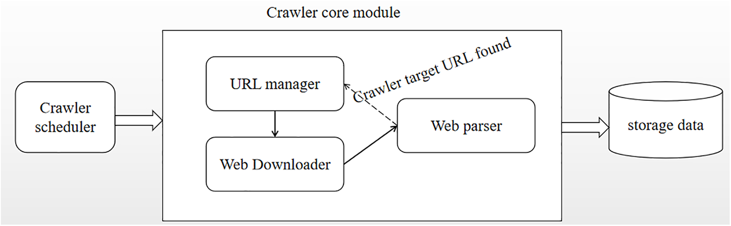
Figure 1: The framework of a web crawler

2.2 Pandas in Python

Pandas is a data processing tool based on the Python language, mainly used for data cleaning, analysis, and visualization. The Pandas module also provides rich data processing tools and functions, making data analysis and processing more efficient and convenient. At the same time, Pandas has good compatibility and can be integrated with other Python modules and tools, such as NumPy, Matplotlib, and more. Therefore, Pandas has become an indispensable important tool in the field of Python data analysis [6]. In addition to routine data processing and analysis tasks, Pandas also supports more advanced application scenarios, such as time series analysis, financial calculations, machine learning, and more. Furthermore, Pandas provides flexible Application Programming Interface (API) and documentation, making it easy for users to learn in-depth and customize development.

3  Construction of Water Quality Data Set

3.1 Water Quality Data Crawling

Water quality data is from the surface monitoring station (http://www.cnemc.cn/). The specific steps for crawling the data are as follows: firstly, enter the developer mode to view the webpage source code and related files to analyze the data interface of the dynamically loaded data; then use the POST request method to extract the required form; finally, change the Pageindex and PageSize parameters to capture all the required information. In this way, we can obtain all the necessary water quality data for subsequent analysis and processing. Some of the water quality data are shown in Fig. 2.

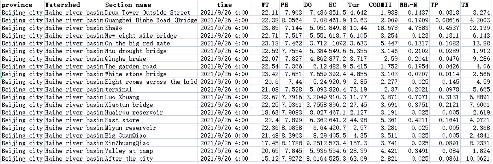
Figure 2: Obtained water quality data

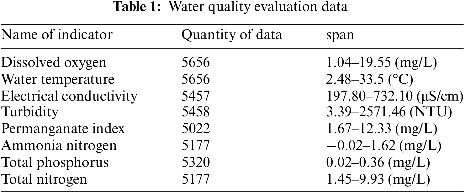
This article selected water quality monitoring sites in a certain watershed as the main research object and imported a total of 5258 water quality monitoring data from July 01, 2018 to January 31, 2021. These data are stored in CSV format on a local computer. The sorted data are shown in Table 1.

3.2 Data Preprocessing

Water quality data has a wide range of sources, a wide range of types, and a large scale of data storage [7]. Due to the large amount of data, it is necessary to store a large amount of real-time monitoring data in a separate business database, so errors will inevitably occur when inputting data. Generally, the better the data quality, the more obvious the characteristics reflected. However, most of the current water quality data sets have problems such as data missing, inconsistent format, outliers, etc., resulting in data quality degradation and “dirty data” [8].

Data preprocessing includes three steps: data cleaning, data conversion and data segmentation, and its flow is shown in Fig. 3. Data cleaning mainly involves filling in missing data and filtering outliers. Data conversion includes normalizing the input sequence to improve the accuracy and efficiency of the algorithm. Data segmentation divides the input sequence into training set and test set to verify the performance and generalization ability of the algorithm.

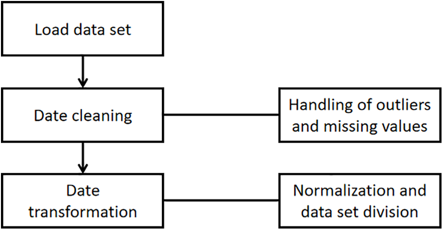
Figure 3: The steps of data preprocessing

3.2.1 Missing Value Processing

The data loss of water quality dirty data can generally be divided into three categories. The first type is scattered data missing. In this case, the proportion of missing values is small. A simple and effective method can be used to directly remove the missing value samples. The second type is the continuous missing of a water quality index, which can be filled by using Lagrange interpolation method. Through the high-order nonlinear fitting of the index, better results can be obtained. The third type is that multiple water quality indicators are missing at different times, and can be filled by linear interpolation, because in this case, linear interpolation can achieve faster filling effect, and the filling effect is not different from that of Lagrange interpolation.

(1) The linear interpolation filling method is often used for one-dimensional data processing. It can establish a linear equation based on the two known values before and after the missing values in the sequence, and fill in the missing values in the time series data through the established interpolation function. In time series data, there is often a certain correlation and trend between data points, and the time span between data points may also be uneven. However, linear interpolation ignores the continuity of the time series, and there are limitations in dealing with continuous missing values.

(2) The Lagrange interpolation method can achieve polynomial nonlinear fitting by establishing single-variable multi-order equations. It can solve the problem that linear interpolation cannot solve the problem of time continuity. Y = g (x) is a polynomial function, and the interval of x is (0, t), where it represents the value of the independent variable at point t, and represents the value of the dependent variable at point t, its formula can be expressed as:

L(x):=∑n=0kynln(x)(1)

lj(x):=∏i=0,i≠nkx−xixn−xi=x−x0xn−x0⋅⋅⋅x−xn−1xn−xn−1x−xn+1xj−xn+1⋅⋅⋅x−xkxn−xk(2)

3.2.2 Outlier and Noise Data Processing

At present, the commonly used outlier detection methods can be divided into two categories. One is based on statistics such as box chart. These methods determine outliers based on the distribution characteristics of data, and can quickly identify and locate outliers. One is clustering method [9], like k-means. This method based on distance and density needs to manually set the cluster size in advance, which can be used to distinguish outliers. According to the data distribution characteristics of turbidity and total phosphorus, this paper selects the clustering method to deal with outliers.

Different situations have different processing methods, and in this paper, we preferred to use Euclidean distance as a reference to analyze the data. The flowchart of the k-means clustering is shown in Fig. 4. The algorithm first selects K data points from the dataset as initial centroids. Then, it calculates the distance between each centroid and the remaining data points, and assigns each data point to the cluster of the nearest centroid. Next, it recalculates the center point of each cluster by taking the mean value of all data points in that cluster. If the distance between the new centroid and the original centroid is significantly different, the process is repeated until the distance is less than a preset threshold. During this process, the position of the new centroid gradually stabilizes, indicating that the clustering has achieved the desired effect. At this point, the algorithm stops [10,11].

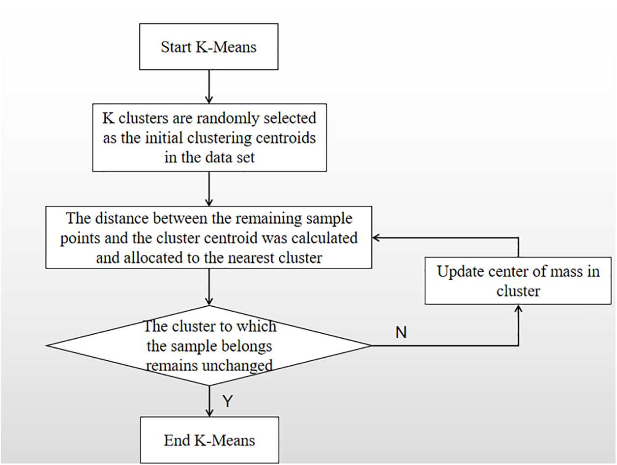
Figure 4: Flow chart of k-means clustering

3.2.3 Data Cleaning

In data preprocessing, The Pandas libraries are called for importing data and converting it to Dataframe. The Pandas library selects total phosphorus data for analysis out of water resources data and filling using linear regression. The effect of data filling with missing values is shown in Figs. 5 and 6.

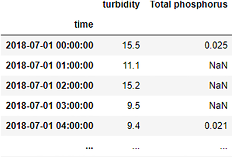
Figure 5: The raw data

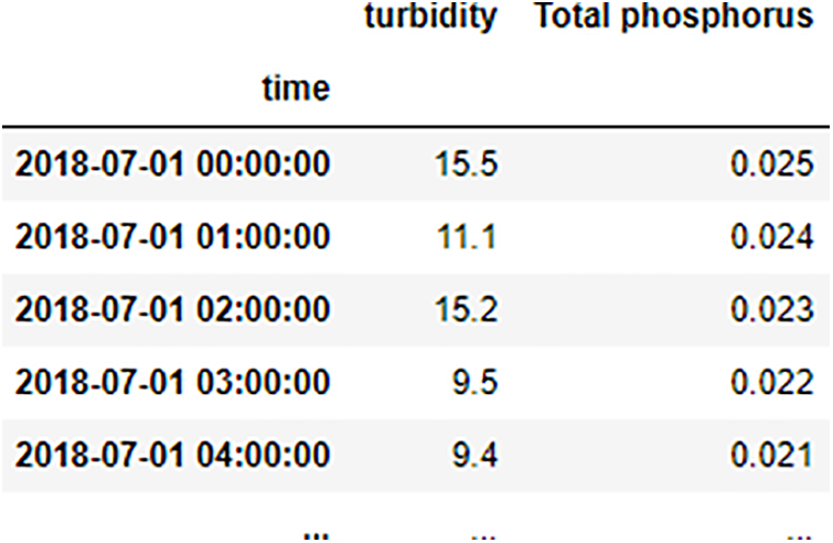
Figure 6: The processed data

The entire analysis is then performed, selectively addressing outliers and outliers in the data collection. The analysis process typically uses the maximum, minimum, mean and the standard deviation that are commonly employed in a statistic to represent the data. A call to panda converts the data to a data frame type then calls library functions to find the appropriate values, making the representation of that data more visual, as illustrated in Table 2.

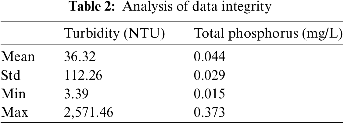
As can be seen from the table above, there are exaggerated data for the maximum values of turbidity and total phosphorus. This can be caused by the long working time and instrument aging, resulting in errors in the data at a specific time point. During the analysis, these values can be considered as outliers. However, the use of box line plots to deal with abnormal values of total phosphorus and turbidity is not effective enough, and some existing normal data will be eliminated. From their scatter plots, it is found that their characteristics are relatively separated and relative. Because of its compactness, the clustering method can be selected to deal with the abnormal value of total phosphorus and turbidity.

This paper calls the Sklearn library in python for machine learning, and uses the k-means method to eliminate outliers from the data. In the Sklearn library, the maximum number of iterations is preset as 300 times, and the distance of the minimum iteration is 0.001. In the process of outlier processing, dividing the data into different numbers of clusters will have different effects on the prediction results. Therefore, when setting the number of clusters, we choose the contour coefficient as the evaluation index of the model. The closer the contour coefficient is to 1, the better the classification effect will be. The contour coefficient obtained is shown in Figs. 7 and 8.

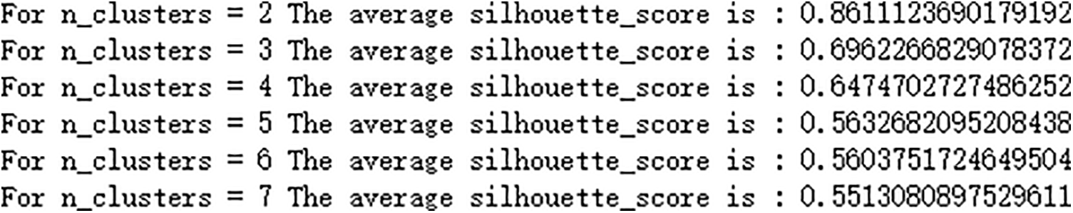
Figure 7: Contour coefficient of total phosphorus

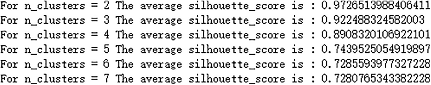
Figure 8: Contour coefficient of turbidity

From the Figs. 7 and 8, we can see that when the number of clusters is 2, the contour coefficients of total phosphorus and turbidity are the highest. Therefore, when we process data through k-means clustering, we can classify the data into two clusters, one is normal value and the other is abnormal value. The effect of clustering is shown in Figs. 9 and 10.

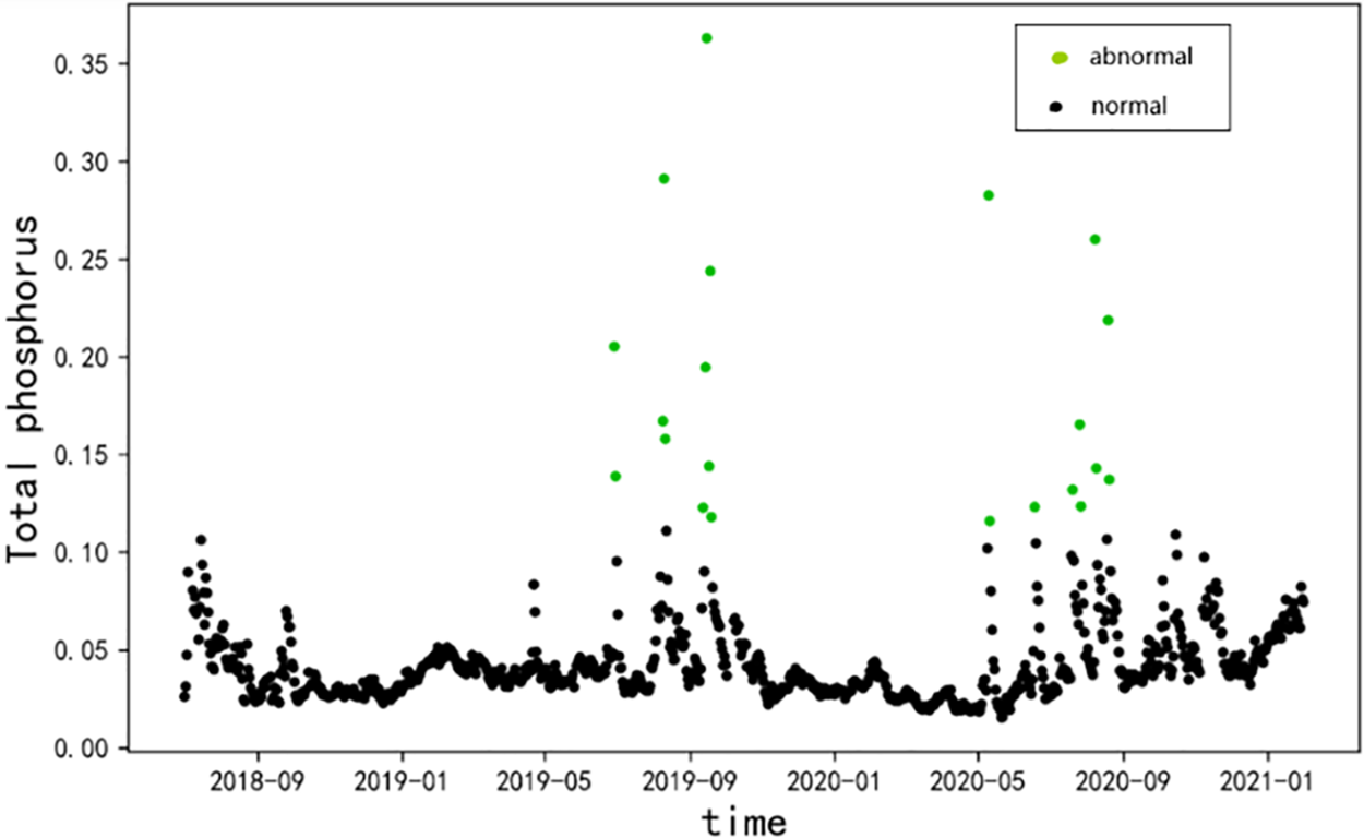
Figure 9: Total phosphorus outlier clustering

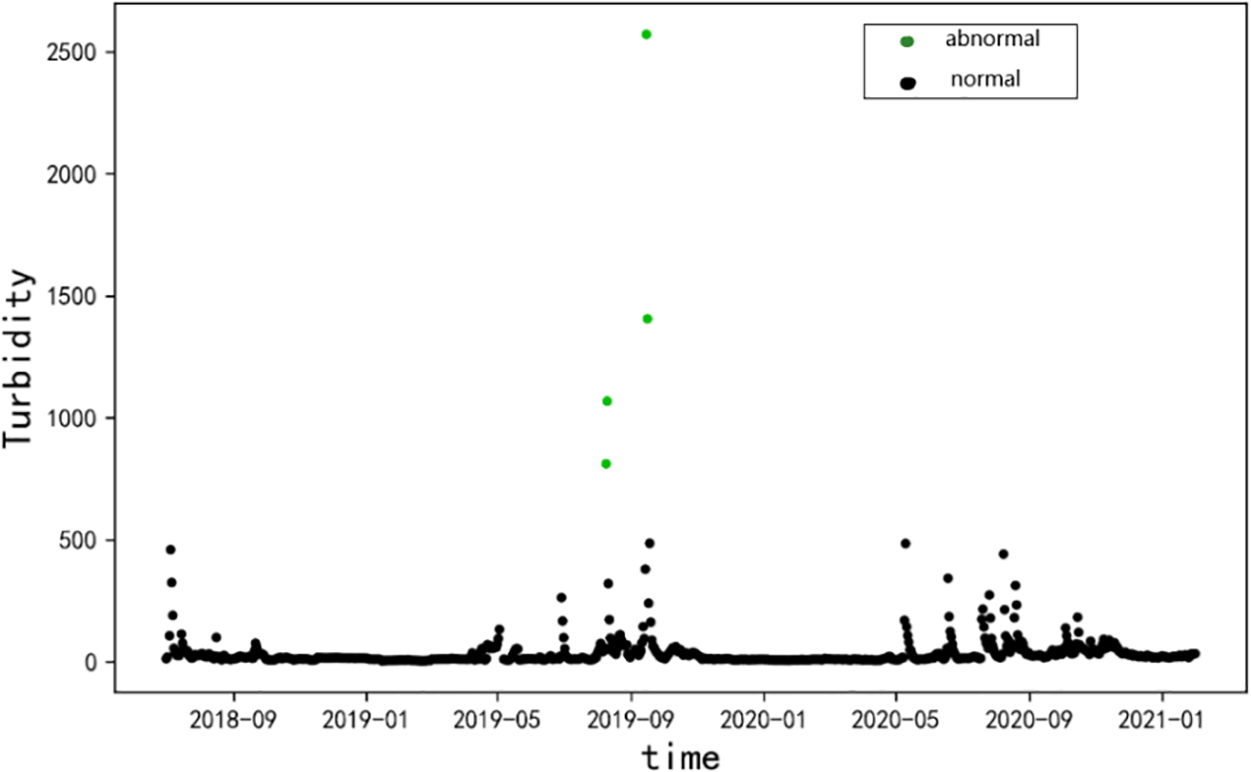
Figure 10: Clustering of turbidity outliers

3.3 Data Transformation

(1) Normalization. In order to eliminate the influence of different units on the prediction results and speed up the convergence of the model, normalization is used in this article [12,13]. By transforming water quality data into a numerical range between 0 and 1, uniform processing of the data is achieved. The specific normalization formula is as follows.

This paragraph is translated into English as follows:

Znorm=Z−ZminZmax−Zmin(3)

where, Znorm represents ote new sequences after normalization, Z represents the input raw sequence, Zmin and Zmax are respectively represent the minimum and maximum values of the input sequence.

(2) Data set partitioning. To ensure that our model performs well and has good generalization ability on the test set, we adopted a data splitting method where the data from July 05, 2018 to January 31, 2021 was divided into training and testing sets in an 8:2 ratio. This approach aims to prevent the model from performing well on the training set but poorly on the test set. By doing so, we can more accurately evaluate the performance and generalization ability of the model, thereby increasing our confidence in its reliability.

4  Correlation Analysis

4.1 Correlation Analysis

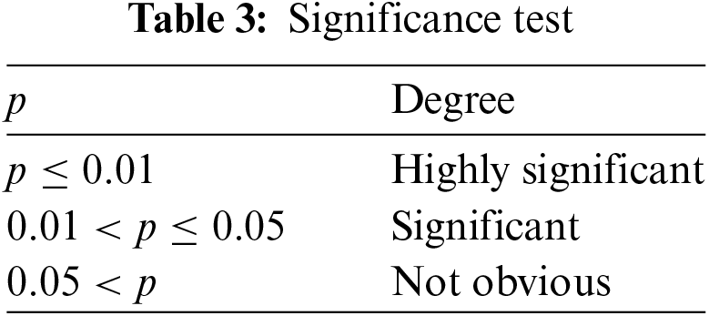
T-test is a common statistical method, which can be used to judge whether there is a significant difference between the mean values of two samples. This method has two forms, namely independent sample T-test and paired sample T-test. Among them, independent sample T-test is applicable to compare whether the mean values of two groups of independent samples are equal; The paired sample T-test is applicable to compare the mean value of the same group of samples under different conditions [14]. The range and significance of p value are shown in the Table 3.

4.2 Visualization Analysis

For reflecting total phosphorus and turbidity under one coordinate system, we have set up a double Y-axis system of coordinates so that both can be represented by the common time series as axes. At the same time, in order to see the total for the relationship between phosphorus and turbidity, we visualized the daily average data and monthly average data of total phosphorus and turbidity after processing the abnormal values. The results are shown in Figs. 11 and 12.

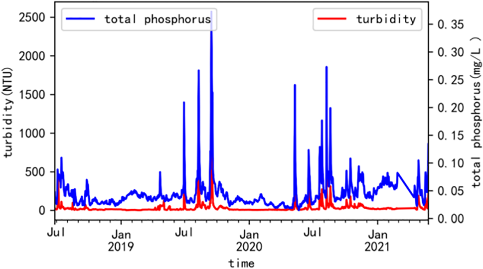
Figure 11: Visualization of daily averages

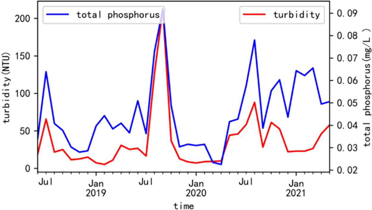
Figure 12: Visualization of monthly averages

As you can see from Fig. 11 that the turbidity and total phosphorus have the same periodic changes, and the two curves almost appear at the highest peaks. It can be seen from Fig. 12 that the change curves of total phosphorus and turbidity are basically consistent, and the two curves are nearly parallel. As the turbidity increased, the concentration of total phosphorus also increased. It can be seen that turbidity is positively correlated with total phosphorus.

4.3 Linear Regression Analysis

In the monthly mean chart of the above time series, we can observe that the variation range of variables is almost the same or opposite to the affected factors. In order to determine the change relationship between variables and influencing factors, we will carry out linear regression analysis and implement it using Scikit-Learn, a special machine learning library widely used in Python. By analyzing the following variables, we can better understand the correlation between them and the influencing factors. The results are shown in Figs. 13 and 14.

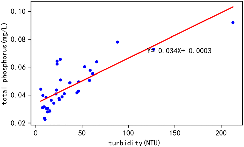
Figure 13: The monthly mean linear regression of turbidity and total phosphorus

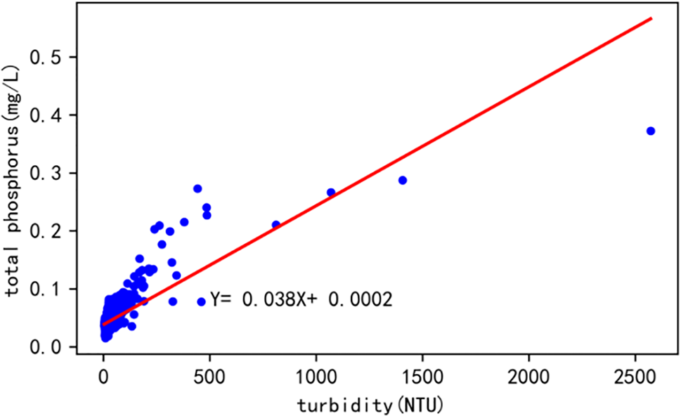
Figure 14: The daily average linear regression between turbidity and total phosphorus

According to the data in Fig. 13, there is a linear regression relationship between the daily average values of turbidity and total phosphorus, and the regression equation is y = 0.034x + 0.0003. In addition, the correlation coefficient between the two variables is 0.77, indicating a strong correlation between them, and the significance probability P < 0.01, indicating that the relationship between the two variables is very significant. Therefore, it can be concluded that there is a negative correlation between turbidity and total phosphorus.

According to the data in Fig. 14, there is a linear regression relationship between the monthly average values of turbidity and total phosphorus, and the regression equation is y = −0.038x + 0.002. In addition, the correlation coefficient between the two variables is 0.77, indicating a strong correlation between them, and the significance probability P < 0.01, indicates that the relationship between the two variables is very significant. Therefore, it can be concluded that there is a negative correlation between turbidity and total phosphorus.

4.4 Water Quality Predicting

In order to validate the feasibility of the model in practice, we will analyze the data for the next 5 days with turbidity as the variable. By using Matplotlib to plot the visualization of the predicted curve and the actual curve, we can intuitively compare the error rate between the predicted values and the actual values. Fig. 15 displays both the predicted curve and the actual curve, allowing for a visual comparison between the two. Table 4 presents a comparison of the error rates between the predicted values and the actual values.

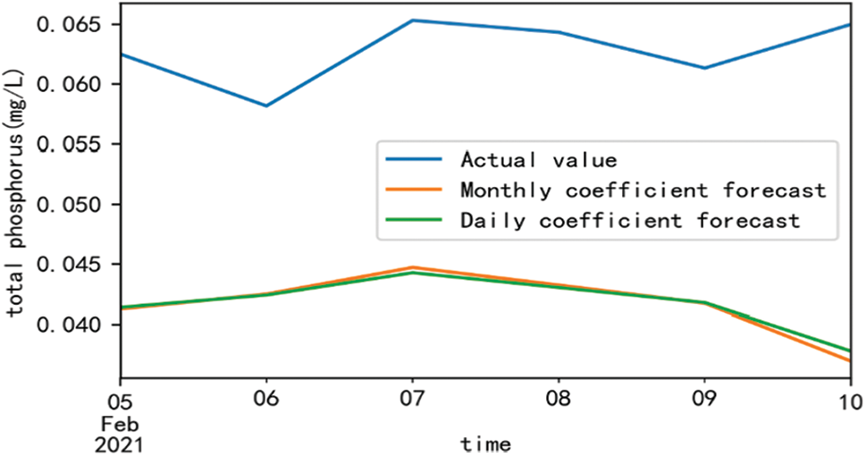
Figure 15: The forecast line is compared with the actual line

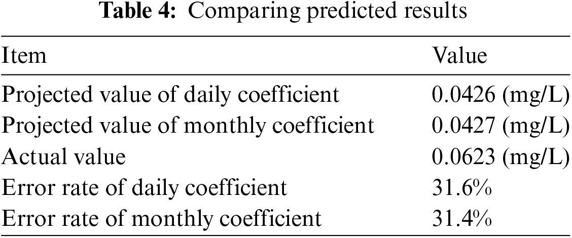
We can draw conclusions from the above Fig. 15 and Table 4:

(1) From the perspective of correlation, total phosphorus and turbidity are highly correlated. However, there are still some errors from the actual error point of view, indicating that in actual prediction, high correlation does not necessarily mean that the prediction is more accurate.

(2) The monitoring of water bodies in the future can be well achieved by observing and predicting curves, which has important practical significance for preventing water pollution accidents and ecological protection.

5  Conclusion

This paper uses water turbidity as a variable to analyze the correlation of total phosphorus. First, relevant features were verified by visual presentation and significance T-test. Secondly, by analyzing the correlation, the linear regression lines of the daily mean and the monthly mean were obtained respectively. Finally, the correlations were used to predict water quality-related variables for the next five days, and a comparison was made between the forecast and the actual value. This prediction of future days’ data through correlation between variables can provide early warning of potential future water quality risks from a predictive point of view, and can provide a foundation for studying the security of regional watershed management. In addition, because of our own standard limitation, we only add single variable factors throughout this paper as correlation analysis, and in the next process, as well as the use of a more advanced elasticity network for the prediction.

Acknowledgement: The authors would like to appreciate all anonymous reviewers for their insightful comments and constructive suggestions to polish this paper in high quality.

Funding Statement: This research was funded by the National Natural Science Foundation of China (No. 51775185), Natural Science Foundation of Hunan Province (No. 2022JJ90013), Intelligent Environmental Monitoring Technology Hunan Provincial Joint Training Base for Graduate Students in the Integration of Industry and Education, and Hunan Normal University University-Industry Cooperation. This work is implemented at the 2011 Collaborative Innovation Center for Development and Utilization of Finance and Economics Big Data Property, Universities of Hunan Province, Open Project, Grant Number 20181901CRP04.

Author Contributions: The authors confirm contribution to the paper as follows: study conception and design: Jianjun Zhang, Ke Xiao, Li Wang, Haijun Lin, Guang Sun and Peng Guo; data collection: Xing Liu, Jiang Wu and Yifu Sheng; analysis and interpretation of results: Wenwu Tan, Jianjun Zhang; draft manuscript preparation: Wenwu Tan, Jianjun Zhang. All authors reviewed the results and approved the final version of the manuscript.

Availability of Data and Materials: These data were derived from the following resources available in the public domain: http://www.cnemc.cn/.

Conflicts of Interest: The authors declare that they have no conflicts of interest to report regarding the present study.

References

1. H. D. Zhou, W. Q. Peng, X. Du and H. J. Huang, “Surface water quality evaluation in China,” Journal of China Institute of Water Resources and Hydropower Research, vol. 2, no. 4, pp. 21–30, 2004. [Google Scholar]

2. X. Zhang, “China’s water pollution trends and governance systems,” China Soft Science, vol. 29, no. 10, pp. 11–24, 2014. [Google Scholar]

3. H. J. Xiao, H. Mou and M. T. Li, “Surface water quality monitoring status and improvement countermeasures,” Times Agricultural Machinery, vol. 45, no. 6, pp. 118, 2018. [Google Scholar]

4. C. Luo, “Design of big data acquisition system based on web crawler technology,” Modern Electronic Technique, vol. 44, no. 16, pp. 115–119, 2021. [Google Scholar]

5. Y. Zhang and Y. Q. Wu, “Design of network data crawler program based on python,” Computer Programming Skills and Maintenance, vol. 27, no. 4, pp. 26–27, 2020. [Google Scholar]

6. C. L. Tang, H. Shen, H. C. Tang and Z. F. Wu, “Research and application of data preprocessing methods in the context of big data,” Information Recording Material, vol. 22, no. 9, pp. 199–200, 2021. [Google Scholar]

7. S. Y. Yin, X. K. Chen and L. Shi, “Data desensitization and visualization analysis based on python,” Computer Knowledge and Technology, vol. 15, no. 6, pp. 14–17, 2019. [Google Scholar]

8. Q. Kong, C. Q. Ye and Y. Sun, “Research on data preprocessing methods for big data,” Computer Technology and Development, vol. 28, no. 5, pp. 1–4, 2018. [Google Scholar]

9. Y. J. Ying, “Big data cleaning method for transmission and transformation equipment status based on time series analysis,” Automation of Power Systems, vol. 39, no. 7, pp. 138–144, 2015. [Google Scholar]

10. Y. Ding and R. X. Li, “Using the data cleaning function of pandas to extract relevant information of broadband users,” Network Security and Informatization, vol. 6, no. 9, pp. 94–96, 2021. [Google Scholar]

11. L. Xu, “Algorithm and application of cluster analysis,” M.S. dissertation, Jilin University, Changchun, China, 2010. [Google Scholar]

12. B. F. Chi, “Research on anomaly detection algorithm based on time series reconstruction,” M.S. dissertation, Beijing Jiaotong University, Beijing, China, 2021. [Google Scholar]

13. J. Y. Liu, H. Xia, Y. Xiang and Y. Shi, “Guizhou tea price forecast based on time series and logistic regression,” Information Technology and Information Technology, vol. 46, no. 7, pp. 70–75, 2021. [Google Scholar]

14. J. Qi and C. L. Zhou, “Correlation analysis between land use pattern and water quality in Hanfeng Lake Watershed of Kaizhou,” Sichuan Environment, vol. 36, no. 1, pp. 58–63, 2017. [Google Scholar]