Near Term Hybrid Quantum Computing Solution to the Matrix Riccati Equations

1  Introduction

Quantum computing is an emerging field which utilizes the principles of quantum physics to perform computations in fundamentally different ways from classical computers. For certain problems, quantum algorithms offer significant improvements in execution time over their classical counterparts. One of the most famous examples is Shor’s algorithm for factoring large (100–200 digit) numbers into the product of two primes, thus making it possible to break modern public-private key encryption schemes [1]. While the theoretical basis of this field has been understood for many decades, only within the past few years have small working quantum computers become available. One of the largest currently available quantum computers is the IBM Q System One, which is programmed using the Qiskit language [2]. Much of the near-term research in this field involves proof of concept implementations, which are limited by the scalability of current quantum computer hardware. Nevertheless, it’s critical to study these applications at a small scale now, in preparation for larger quantum computers becoming available within the next few years (current systems are limited to a handful of qubits; however, IBM roadmaps plan for a 1,000-qubit machine by 2024 or sooner [3]). For example, IBM has recently announced quantum resistant encryption features on the latest model z16 enterprise server [4], even though we are years away from building a large enough quantum computer to seriously threaten conventional encryption.

While there are currently only a few known examples where quantum computers offer a potential performance advantage, one promising area is the solution of systems of linear differential equations. For this problem, it has been shown [5] that under certain conditions, quantum algorithms can yield an exponential improvement in execution time compared with the best-known classical algorithms. In this paper, we investigate the use of quantum algorithms to generate approximate solutions to systems of nonlinear differential equations. Our approach involves a transformation which turns a set of nonlinear differential equations into an approximation using linear differential equations with second order non-constant coefficients. We can then solve a matrix representing this set of linear differential equations using a version of the Harrow-Hassidim-Lloyd (HHL) quantum algorithm, for the common case of Hermitian matrices.

Specifically, we are interested in the well-known Matrix Riccati nonlinear differential equations [6], which play a role in a wide range of fields including problems in protein folding, control and stabilization, stochastic control, and cybersecurity (risk analysis and malware propagation) [7–10]. These equations have been studied extensively using classical computing techniques, including significant efforts by national research labs [11], and approximate solutions with varying degrees of accuracy have been demonstrated. We propose a novel hybrid quantum-classical algorithm, the Matrix Riccati Solver (MRS), which is implemented on a near-term 4 qubit quantum computer using Qiskit. We then compare the accuracy achievable with the MRS and conventional approaches over a limited neighborhood of values. It is possible to achieve useful accuracy with this approach, and future quantum computers with additional qubits are expected to offer even better performance.

The remainder of this paper is organized as follows. Following a short introduction, we describe the fundamental Riccati equation formulations, the quantum linear systems problem, and the HHL algorithm. We then describe our implementation of the MRS hybrid algorithm, and present experimental results running on a 4-qubit quantum computer. We compare the MRS results with the best available classical approximations and suggest areas for further research.

2  Riccati Equations Fundamentals

In general, a Riccati equation is any first order ordinary differential equation that is quadratic in the unknown function, such as equations of the form

y′=a(t)⋅y2+b(t)⋅y+c(t)(1)

where a(t), b(t) and c(t) are nonzero, continuous functions of t. More generally, the term Riccati equation is used to refer to matrix equations with an analogous quadratic term, which occur in both continuous-time and discrete-time linear quadratic Gaussian control systems. The steady-state (non-dynamic) version of these is referred to as the algebraic Riccati equation. The non-linear Riccati equation can always be converted to a second order linear ordinary differential equation (ODE).

To date, there is no general approach for finding solutions to the Riccati equations, although there are analytical techniques which allow solutions under certain conditions as well as numerical approximation solutions for other cases. For example, suppose we have a particular solution y1 to this general equation. Then we can make the following change of variables

y=y1+u(2)

and so, we can rewrite the general equation as

(y1+u)′=a(t)⋅(y1+u)2+b(t)⋅(y1+u)+c(t)(3)

y1′+u′=a(t)⋅(y12+2⋅y1⋅u+u2)+b(t)⋅y1+b(t)⋅u+c(t)(4)

y1′+u′=a(t)⋅y12+a(t)⋅2⋅y1⋅u+a(t)⋅u+b(t)⋅u+b(t)⋅y1+c(t)(5)

It follows that, since y1 is a particular solution to the Riccati equation we can cancel out y1′,a(t)⋅y12,bt⋅y1, and c(t). Hence, we obtain

u′=a(t)⋅u2+u⋅(2⋅a(t)⋅y1+b(t))(6)

u′−u⋅(2⋅a(t)⋅y1+b(t))=a(t)⋅u2(7)

u′−u(2⋅a(t)⋅y1+b(t))u2=a(t)(8)

Note that u′ is a Bernoulli equation and thus we can apply well-established methods to find the general solution. First, we make the substitution z = u1−m, where m = 2 in this case, to transform the Bernoulli into the following linear differential equation:

−z′−(2⋅a(t)⋅y1+b(t))⋅z=a(t)(9)

We will expand these methods to a matrix formalism, which is the standard approach used in quantum computing state machines.

3  Quantum Linear Systems Problem

The “Classical” Linear System Problem (LSP) states the following:

Given an N × N matrix A, an N–dimensional vector b→ and the equation

A⋅x→=b→(10)

Solve for x→ = (x1, x2, … , xN)T. To date, the best algorithm for this task is called the Conjugate Transpose method, first introduced by Hestenes et al. in 1952 [12]. It has an asymptotic complexity of O(N⋅k) and thus, complexity grows in polynomial time as the number of inputs increases.

Analogously, the Quantum Linear System Problem (QLSP) states that given a Hermitian Given an N × N matrix A, an N –dimensional vector b→, and the equation

A⋅x→=b→(11)

Prepare a quantum state that approximates the column vector

x→=∑i=1Nxi⋅i→∑i=1N|xi|2(12)

where x→=(x1,x2,…,xN)2. Specifically, for a given precision ϵ>0, the approximate (mixed or pure) quantum state ρx satisfies

12⋅Tr|ρx−xT→⋅vecx|≤ϵ(13)

4  The HHL Algorithm

The Harrow-Hassidim-Lloyd (HHL) quantum algorithm [3] may be applied to expressions like those we developed in the previous section. Given a Hermitian matrix A, the HHL algorithm will compute the vector of unknowns x→ in the form

x→=∑j=1Nβj⋅1λj⋅uj→(14)

where {u→j} denotes the eigenvectors of A and {λj} its eigenvalues. Then, HHL performs three important operations:

•   Quantum Phase Estimation (QPE)

•   Invert the eigenvalues

•   Measurement

QPE is a central building block for many quantum algorithms. As shown in the quantum circuit of Fig. 1, QPE estimates the phase of an eigenvalue of the unitary operator U that we create by using the properties of Hermitian matrices. Given a unitary operator, U, QPE estimates the phase angle theta in

U⋅ψ→=e2⋅π⋅i⋅ψ→(15)

where ψ→ is an eigenvector (i.e., state vector) and e2⋅π⋅i⋅ψ→ is the eigenvalue. Note that since U is a unitary operator, all eigenvalues have a norm of 1.

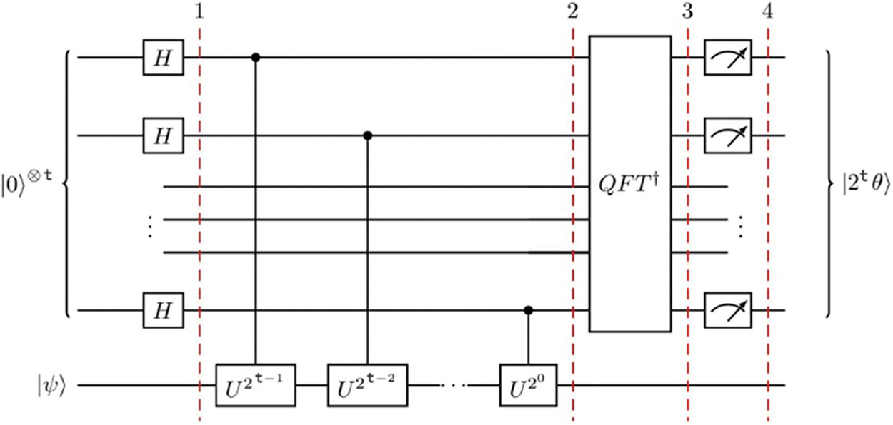
Figure 1: Quantum Phase Estimation (QPE) circuit using quantum fourier transform (QFT), hadamard gates (H), and various unitary transforms (U)

A quantum circuit for this algorithm is shown in Fig. 2, incorporating the QPE circuit from Fig. 1 and leveraging the lin_alg package from Qiskit so that we can treat the HHL algorithm as a black box.

Figure 2: Quantum circuit for the HHL algorithm

After encoding the solution vector b→ as a linear combination of the input matrix A’s eigenvectors, the algorithm undergoes an iterative process of computing the inverse of A’s eigenvalues, by applying Quantum Phase Estimation with U = ei⋅A⋅t, and its inverse until the measurement (depicted between demarcation lines 4 and 5 of Fig. 2) yields 1. Then, it returns the estimated solution

x→=∑j=1nujT→⋅b→λj⋅uj→(16)

5  The Matrix Riccati Solver (MRS)

We propose a hybrid algorithm, the Matrix Riccati Solver (MRS), to find solutions for the matrix form of these equations given a set of initial conditions. First, we show that some Matrix Riccati equation can be re-written as a Hermitian matrix, given certain conditions are met, and encode this fact in the classical component of the proposed algorithm. Then, we feed the Hermitian matrix to HHL on IBM’s 4-qubit near-term quantum computer to obtain the solution.

Let R denote the following Matrix Riccati equation

Y′=Y⋅A(t)⋅Y+C(t)⋅Y+Y⋅B(t)+D(t)(17)

where Y ∈ ℝn × m, D(t) ∈ ℝn × m, C(t) ∈ ℝn × n, B(t) ∈ ℝm × m and A(t) ∈ ℝm × n. The goal is, given an initial condition Y(0), to obtain solutions Y(t), ∀ t > 0.

We propose the following theorems (see Appendix for full proof):

Theorem 1: Assuming m = n, if B(t) = 0 and if A(t) is invertible, then Eq. (17) can be converted to the following second order matrix differential equation:

u″−(ACA−1+A′A−1)⋅u′+AD⋅u=0(18)

By using the change of variables Y = − A−1 ⋅ u′ ⋅ u−1, where u is invertible.

Theorem 2: If ACA−1 + A′A−1 = S where S is a matrix with constant entries and diagonalizable, and

A ⋅ D = −I , then (18) can be converted into the following equations:

v″−D1⋅v′−v=0(19)

where D1 is a diagonal matrix.

From (18) we derive the following linear system

e−tMii⋅xii=wii(SeeAppendix)(20)

where M11 = 0, M12 = 1, M21 = 1, M22 = −αi, and αi denotes the entries in the diagonal matrix D1,

wii = [vii (0), v′ ii (0)]T, where vij are the entries of v so v = (vij) and 1 ≤ i, j ≤ n .

Solving (20) is equivalent to solving the system

H⋅x→=w→(21)

where x→=(x11,x22,…,xnn)T, H has diagonal entries are Hij=e−t⋅Mnn and w→=(w11,w22,…,wnn)T. Note that H is sparse and Hermitian for any i. Thus, we can leverage the HHL algorithm once we normalize the vector w→. In the particular case where m = m = 1, we get the following Riccati equation:

dy/dt=A(t)⋅y2+B(t)⋅y+C(t)(22)

where A(t), B(t), C(t) are real-valued functions of t. We seek to compute y(t) given an initial condition y(0). We convert the Riccati equation to a second order differential equation by applying the change of variables

y=−v′A⋅v(23)

Such that we obtain the following equation:

v″−v′⋅(B+A′A)+A⋅C⋅v=0(24)

Next, let α=B+A′A and assume A ⋅ C = −1, which must hold for the resulting matrix to be Hermitian.

From this, we obtain a system with vector of unknowns u→ = (v, z )T and a matrix M M11 = 0, M12 = 1, M21 = 1, M22 = −α. Therefore, we obtain the following equation u′ = M ⋅ u. We proceed by computing the characteristic polynomial to obtain the following eigenvalues

λi=α±α2+42,i∈{1,2}(25)

and thus, the corresponding eigenvectors are:

Vi=(1,λi)T(26)

Finally, we construct a 2 × 2 passage matrix P = (V1, V2), such that we can rewrite our matrix M as H = P ⋅ D ⋅ P−1 where D is a diagonal matrix with entries λi.

It follows that to solve this system we must compute x→=etH⋅x→0→ where x→0→= (u(0), z(0))T. Thus, we must rewrite the problem as e−tH ⋅ x→ = x→0→, where e−tH = P ⋅ e−tD ⋅ P−1. Since we now know e−tH is Hermitian, we conclude by normalizing x→0→ such that u(0)2 + z(0)2 = 1. Fig. 3 is a high-level pseudocode description of the algorithm.

Figure 3: Matrix Riccati Solver (MRS) algorithm’s pseudocode

The MRS checks that the required conditions are met. If not, the program displays an error and halts. To ensure that α is a constant MRS checks its derivative equals zero and then registers the variable as a constant quantity using the Python package SimPy constant quantity [13]. Then, MRS computes the eigenvalues λi of the system of equations we derived in the previous section. The eigenvalues are then utilized to compute the values of each component in our new matrix . We solve for M⋅x→=b→ to compute the normalized vector of unknowns x→ for the specified initial condition Y(0) by calculating the values of its components

x011+A(0)2+Y(0)2(27)

x1=A(0)⋅Y(0)1+(0)2+Y(0)2(28)

We can then input M and x→ to HHL to find the solution to the given system. This is achieved by extracting the state vector ψ, containing the quantum state of each qubit, from the circuit generated by the quantum computer. Finally, MRS extracts the states of the qubits containing our answers and computes a numeric approximation of the solution by solving for which denotes the time for which we are evaluating the expression. The initial condition refers to the value y(T = 0).

yt=−(z(T)(A(T)⋅u(T)))(29)

6  Experimental Results

To test the algorithm’s performance, we used the following example. Consider the following Riccati equation with initial condition y(0) = 1

dydt=(2−sin(t))⋅y2+2−sin(t)+cos(t)2−sin(t)⋅y−12−sin(t)(30)

Recall the Uniqueness and Existence theorem [2] states that there is a unique solution for a given initial value problem within a local neighbourhood, defined by ε > 0 . Fig. 4 shows the results of both the quantum solution (i.e., Matrix Riccati Solver) and classical solution over the local neighborhood (0.30, 0.38) with a time step of 0.001.

Figure 4: Comparison of classical solution and hybrid quantum-classical MRS solution

The accuracy of the quantum algorithm varies from a nearly exact solution near the edges of this neighborhood to a worst-case error of −1.444 at T = 0.3570. For some applications this is an acceptable error tolerance; in other cases, such as risk assessment analysis, the quantum algorithm will slightly under-estimate risk factors over this neighborhood. This error is likely attributed to the relatively small number of qubits used in the near-term approximate solution. Although there will always be some error due to quantum fluctuations, future quantum computers are expected to provide a better approximation of the classical solution over a larger neighborhood.

7  Conclusion

We propose a hybrid classical-quantum algorithm to generate solutions to nonlinear differential equations, specifically the Riccati equations, by approximating them as a series of linear differential equations. Previous research indicates that quantum assisted solutions should provide an exponential speedup in execution time. Although this may not be fully realized using near-term quantum computers, we investigate algorithms which can be scaled to larger numbers of qubits in future systems. Near term results indicate that over neighborhoods of interest the hybrid MRS algorithm offers good accuracy for a number of applications. Additional research is planned to investigate larger quantum computers as they become commercially available.

Acknowledgement: We would like to thank the Mathematics and Computer Science department at Marist College for supporting our academic endeavors with insightful conversations and advice.

Funding Statement: The authors received no specific funding for this study.

Conflicts of Interest: The authors declare that they have no conflicts of interest to report regarding the present study.

References

1. P. Shor, “Polynomial time algorithms for prime factorization and discrete logarithms on a quantum computer,” SIAM Journal on Computing, vol. 26, no. 5, pp. 1484–1509, 1997. https://doi.org/10.1137/S0097539795293172 [Google Scholar] [CrossRef]

2. A. Asfaw, L. Bello, Y. Ben-Haim, S. Bravyi, N. Bronn et al., “Learn quantum computing using Qiskit,” 2020. [Online]. Available: https://community.qiskit.org/textbook [Google Scholar]

3. J. Hruska, “IBM unveils quantum roadmap, plans 1,000 qubit chips by 2023,” English. 2020. Available: https://www.extremetech.com/computing/315020-ibm-unveils-quantum-roadmap-plans-1000-qubit-chip-by-2023 [Google Scholar]

4. IBM, “Announcing IBM z16: Real-time AI for Transaction Processing at Scale and Industry’s First Quantum- Safe System,” 2022. Available: https://newsroom.ibm.com/2022-04-05-Announcing-IBM-z16-Real-time-AI-for-Transaction-Processing-at-Scale-and-Industrys-First-Quantum-Safe-System? [Google Scholar]

5. A. W. Harrow, A. Hassidim and S. Lloyd, “Quantum algorithm for linear systems of equations,” Physical Review Letters, vol. 103, no. 15, pp. 150502, 2009. https://doi.org/10.1103/PhysRevLett.103.150502 [Google Scholar] [PubMed] [CrossRef]

6. R. Haberman, “Applied Partial Differential Equations with Fourier Series and Boundary Value Problems,” in English, 5th ed., London, UK: Pearson, 2018. [Google Scholar]

7. A. Mohammadi and M. Spong, “Quadratic optimization based nonlinear control for protein conformation prediction,” IEEE Control Systems Letters, vol. 6, pp. 2755–2760, 2022. https://doi.org/10.1109/LCSYS.2022.3176433 [Google Scholar] [CrossRef]

8. A. Anees and I. Hussain, “A novel method to identify initial values of chaotic maps in cybersecurity,” Symmetry, vol. 11, no. 2140, 2019. https://doi.org/10.3390/sym11020140 [Google Scholar] [CrossRef]

9. W. Zhongru, L. Chen, S. Song, C. Pei Xin and R. Qiang, “Automatic cybersecurity risk assessment based on fuzzy fractional ordinary differential equations,” Alexandria Engineering Journal, vol. 59, no. 4, pp. 2725–2731, 2020. [Google Scholar]

10. L. Lystad, N. Per-Ole and H. Ralph, “The Riccati equation–an economic fundamental equation which describes marginal movement in time,” Modeling, Identification and Control, vol. 27, no. 1, pp. 3–21, 2006. https://doi.org/10.4173/mic.2006.1.1 [Google Scholar] [CrossRef]

11. Lawrence Livermore National Laboratory research brief, “NSDE: Nonlinear solvers and differential equations,” 2005. [Online]. Available: https://computing.llnl.gov/projects/nsde (accessed on 08/20/2022). [Google Scholar]

12. M. Hestenes and E. Stiefel, “Methods of conjugate gradients for solving linear systems,” Journal of Research of the National Bureau of Standards, vol. 49, no. 6, pp. 409, 1952. https://doi.org/10.6028/jres.049.044 [Google Scholar] [CrossRef]

13. A. Meurer, M. Paprocki, C. P. Smith, O. Čertik, S. B. Kirpichev et al., “SymPy: Symbolic computing in Python,” PeerJ Computer Science, vol. 3, no. 3, pp. e103, 2017. [Google Scholar]

Appendix

Let R denote the following Matrix Riccati equation

Y′=Y⋅A(t)⋅Y+C(t)⋅Y+Y⋅B(t)+D(t)(A1)

where Y ∈ ℝn × m, D(t) ∈ ℝn × m, C(t) ∈ ℝn × n, B(t) ∈ ℝm × m and A(t) ∈ ℝm × n.

Theorem 1: Assume m = n. If B(t) = 0 and if A(t) is invertible, then (R) can be converted to the following second order differential equation:

u″−(A⋅C⋅A−1+A′⋅A−1)⋅u′+A⋅D⋅u=0(A2)

By using the change of variables Y = −A−1 ⋅ u′ ⋅ u−1, where u is invertible.

Proof.

Y′=−(A−1)′⋅u′⋅u−1−A−1⋅u″⋅u−1−A−1⋅u′⋅(u−1)′(A3)

Recall (A−1)′ = − A−1 ⋅ A′ ⋅ A−1. Then,

Y′=A−1⋅A′⋅A−1⋅u′⋅u−1−A−1⋅u″⋅u−1+A−1⋅u′⋅u−1⋅u′⋅u−1(A4)

Y′=A−1⋅u′⋅u−1⋅A⋅A−1⋅u′⋅u−1+A−1⋅u′⋅u−1⋅B−C⋅A−1⋅u′⋅u−1+D(A5)

It follows that, since B(t) = 0

Y′=A−1⋅u′⋅u−1⋅A⋅A−1⋅u′⋅u−1−C−A−1⋅u′⋅u−1+D(A6)

and so

A−1⋅A′⋅A−1⋅u′⋅u−1−A−1⋅u″⋅u−1=−C⋅A−1⋅u′⋅u−1+D(A7)

By right multiplying by u we get

A−1⋅A′⋅A−1⋅u′−A−1⋅u″=−C⋅A−1⋅u′+D⋅u(A8)

Then, left multiply by A

A′⋅A−1⋅u′=−A⋅C⋅A−1⋅u′+A⋅D⋅u(A9)

Which yields

u″−(A⋅C⋅A−1+A′⋅A−1)⋅u′+A⋅D⋅u=0(A10)

Theorem 2: If A ⋅ C ⋅ A−1 + A′ ⋅ A−1 = S , where S is constant and diagonalizable, and A ⋅ D = − I.

Then, (A1) can be converted to the following equation

v″−D1⋅v′−Y=0(A11)

where D1 denotes a diagonal matrix.

Proof.

We know the S is diagonalizable, thus we can rewrite it as S = P ⋅ D1 ⋅ P−1 where P denotes the passage matrix P−1 ⋅ S = D1 ⋅ P−1. Next, let F denote the following equation:

u″−S⋅u′−u=0(A12)

By left multiplying both sides by P−1 we get

P−1⋅u″−P−1⋅S⋅u′−P−1⋅u=0(A13)

or

P−1⋅u″−D1⋅P−1⋅u′−P−1⋅u=0(A14)

Finally, let v = P−1 ⋅ u which yields

v″−D1⋅v′−v=0(A15)

Obtaining the system from (A15)

Let αi denote the eigenvalues of D1 , where 1 ≤ i ≤ n. Then, the diagonal entries of D1 are Di = αi.

Next, let Vij ∈ ℝ, 1 ≤ i ≤ n and 1 ≤ j ≤ n be the entries of v. Then, (A15) leads to

vij″−αi⋅vij′−vij=0(A16)

Now, notice that vii = vij since αi does not depend on j. Thus, we get

vii″−αi⋅vii′−vii=0(A17)

Next, let wii=vii′ and wii′=vii′=vii+αi⋅wii. Then, let xii→=(vii,wii)T denote the vector unknowns. We can rewrite this as the following system of equations:

dxii→dt=Mii⋅xii→(A18)

To find the solution to (A18) we solve for e−t⋅Mii⋅xii→=x0ii where Mii = (c1, c2), c1 = (0, 1)T, c2 = (0, αi)T, and x0ii denotes the initial value of xii→ .

Computing e−tMi

Let λi denote an eigenvalue of Mii, given by det(Mii−λi⋅I)=0. It follows that λi=αi±αi2+42. Hence, we have two eigenvalues λi1=αi+αi2+42 and λi2=αi−αi2+42, with corresponding eigenvectors wi1=(1,λi1)T and wi2=(1,λi2)T. Then, the passage matrix Pi is given by Pi=(wi1wi2). So, Mii=Pi⋅Ni⋅Pi−1, where Ni is a diagonal matrix with entries λik,k∈{1,2}.

If we multiply both sides by -t and exponentiate we obtain the following equation

e−t⋅Mii=Pi⋅e−t⋅Ni⋅Pi−1(A19)

And therefore the following matrix:

e−t⋅Mii=(λi2⋅e−t⋅λi1−λi1⋅e−t⋅λi2λi2−λi1−e−t⋅λi1+e−t⋅λi2λi2−λi1−e−t⋅λi1+e−t⋅λi2λi2−λi1λi1⋅e−t⋅λi1−λi2⋅e−t⋅λi2λi2−λi1)(A20)

Normalizing the solution vector

For the input system to be valid, HHL requires that the solution vector b→=x0ii=(vii(0),wii(0))T is normalized such that vii(0)2+wii(0)2=1.

Let v=P−1⋅u,vij=∑k=1nPik⋅ukj,w′=vij′,P−1=Pij and u=uij. Then,

vij(0)=∑k=1nPik⋅ukj(0)(A21)

wij(0)=∑k=1nPik⋅ukj′(0)(A22)

Since Y=−A−1⋅u′⋅u−1 we know that

A(0)⋅Y(0)⋅u(0)+u′(0)=0(A23)

u′(0)=−A(0)⋅Y(0)⋅u(0)(A24)

Expressed as sums instead of matrix notation

uki′(0)=−∑l=1n∑s=1nαkl(0)⋅Yls(0)⋅ysi(0)(A25)

vii(0)=−∑k=1nPik⋅uki(0)(A26)

wii(0)=∑k=1nPik⋅(−∑l=1n∑s=1nαkl(0)⋅Yls(0)⋅ysi(0))(A27)

We know apply the normalization condition vii2+wii2=1n,1≤i≤n, and obtain

(−∑k=1nPik⋅uki(0))2+(∑k=1nPik⋅(−∑l=1n∑s=1nαkl(0)⋅Yls(0)⋅ysi(0)))2=1n(A28)

where Pij denotes the entries of the inverse of the passage matrix of S=A⋅C⋅A−1+A′⋅A−1.

Putting everything together yields the solution y(t)=−A−1(T)⋅u′(T)⋅u−1(T), which is the equation plotted in the results sections.