Comparative Study of CPLEX and D-Wave for Track Finding Resolution

1  Introduction

In the beginning of particle physics, techniques for observing particles were developed alongside the theoretical understanding of their behavior, and the earliest methods relied on optical observation of particle trajectories which were recorded through photography. One of the first tracking detectors was the cloud chamber, invented by Wilson in 1910. In this device, particles pass through supersaturated water or alcohol vapor, where the electron-ion pairs along their paths act as condensation nuclei. In 1952, D. Glaser (awarded the Nobel Prize in 1960) invented the bubble chamber, where particles traverse a superheated liquid, and the energy they deposit creates visible bubbles. In both cases, the trajectory of the particle is revealed to the experimenter by a succession of points in space with variable density along the particle track which, when connected by lines, approximate the continuous path followed by the particle.

A single collision between two protons from the two opposite beams of particles at the Large Hadron Collider (LHC) [1,2] can produce thousands of new particles. The collision points can be identified with relatively precise coordinates using detectors, whose innermost components consist of multiple layers of silicon sensors arranged in cylindrical symmetry around the beam tube. This results in a significant computational challenge in reconstructing the trajectories of charged particles, starting from the small energy deposits in the detector, a process known as track finding.

With the High-Luminosity LHC (HL-LHC) [3], the collisions are designed to generate an even greater number of particles, further complicating the calculations due to the limited computational resources available with classical computers.

Particle track reconstruction has raised, with time, significant attention, leading to the development of numerous methods [4,5], including those based on the Likelihood Method. This approach leverages likelihood calculations to determine the most probable tracks and has been extended to define techniques such as the Corridor Method and Tukey weighting. When tracks are linear or exhibit minimal curvature, basic linear track-finding methods can suffice. However, more complex scenarios may require searching for space points connected in sequences, which has led to the development of the Topological Track Finder, capable of identifying both straight and curved tracks. From a practical perspective, physicists often utilize database search algorithms, and methods based on template track finding are employed in all modern detector experiments. The recent advancements in quantum computing have introduced a new paradigm in particle physics, offering the potential for unprecedented speedups. Recently, Brown et al. [6] demonstrated a proof-of-concept quantum algorithm that leverages Grover’s algorithm using Associative Memory.

Over the past decade, a significant amount of research has aimed to achieve a balance between algorithm efficiency and reasonable CPU resource demands. The track-finding algorithm used in the Belle II experiment at the SuperKEKB B-factory in Tsukuba, Japan, is an example of this approach [7]. A very similar approach based on cellar automaton has been introduced in [8]. Concern about CPU resource requirements has led researchers to leverage AI-based methods, including neural networks. These methods offer two key advantages: first, they enable predictions to be computed in relatively short computation times, and second, they excel at modeling complex, non-linear data dependencies, which is crucial for accurately identifying all tracks [9]. Numerous state-of-the-art techniques have been published recently, including those by [4], the very nice introduction in the dissertation of [10], and the state of the art of [11].

Quantum computing, an ambitious and rapidly evolving technology, offers the potential for exponential speedups. Current quantum devices, such as D-Wave quantum computers, can support up to several thousand qubits. Some researchers suggest that by leveraging the power of D-Wave quantum computers and their quantum annealing capabilities [12], it may be possible to significantly reduce the computational time required to solve the track-finding problem [7].

The number of publications addressing the comparison between quantum and non-quantum techniques remains relatively limited (see for example [13] for consideration of complexity), and the number of publications proposing numerical evaluations is even lower, as the performance of quantum machines only allowed tests on very small instances. Despite the progress made, current quantum machines still do not allow studies on large instances.

However, we will show that, in the particular case of track-finding, one of the fundamental problems can be used to calibrate, compare, and objectively evaluate performance. Our proposal follows in the continuity of the reflections put forward by [14,15]. However, while Ref. [14] is limited to a few numerical elements, we aim to provide a more comprehensive numerical study that could serve as a basis for future comparative work defining a new step in the definition of standardized benchmarks [16] within a scientific community which has been proved to have a positive impact in the scientific community for decades [17].

Generally speaking, the scientific community has been interested for several years in comparing classical and quantum solutions, which raises broader questions about comparing QPUs and CPUs, as highlighted in [18]. From this perspective, our contribution represents a first step toward addressing this type of question for a specific optimization problem.

In this paper, we propose a numerical experiment based on Peterson’s cost formula [19], using both a Quadratic Constrained Binary Model (QCBM) and a Quadratic Unconstrained Binary Model (QUBM). These models are solved using a quantum approach with D-Wave and a classical approach with CPLEX, along with a Binary Linear Program (BLP) solved purely with CPLEX. We have created a dataset extracted from the TrackML Kaggle challenge, containing data simulated using ACTS (A Common Tracking Software) [8]. We define a set of instances, including 10 small-scale instances (with 70 to 700 hits), 10 medium-scale instances (with 875 to 2450 hits), and 10 large-scale instances (with 2625 to 4200 hits). The instances and numerical experiments are available at the following web page https://perso.isima.fr/~lacomme/track_finding/data.html (accessed on 15 May 2025) and aim to support fair and impactful future research on the topic.

The paper is organized as follows: Section 2 describes the construction of the QCBM model and its evolution into the QUBM and BLP models. Section 3 outlines the creation of the new instances based on key observations. Finally, Section 4 presents the results of applying our methods to these instances.

2  Models for the Track Finding Problem

2.1 Description

In our study we fix the number L of layers in the detector to 7. By HS=[h1,h2,…,hi,…,hN] we denote the ordered list of hits in all layers. A track is a set of consecutive segments, with a segment created by two hits on two different layers. Let us note that a track can be composed of hits of two non-consecutive layers, since some high energy particles can miss leaving a recordable trace in some layers. A track candidate is illustrated in Fig. 1.

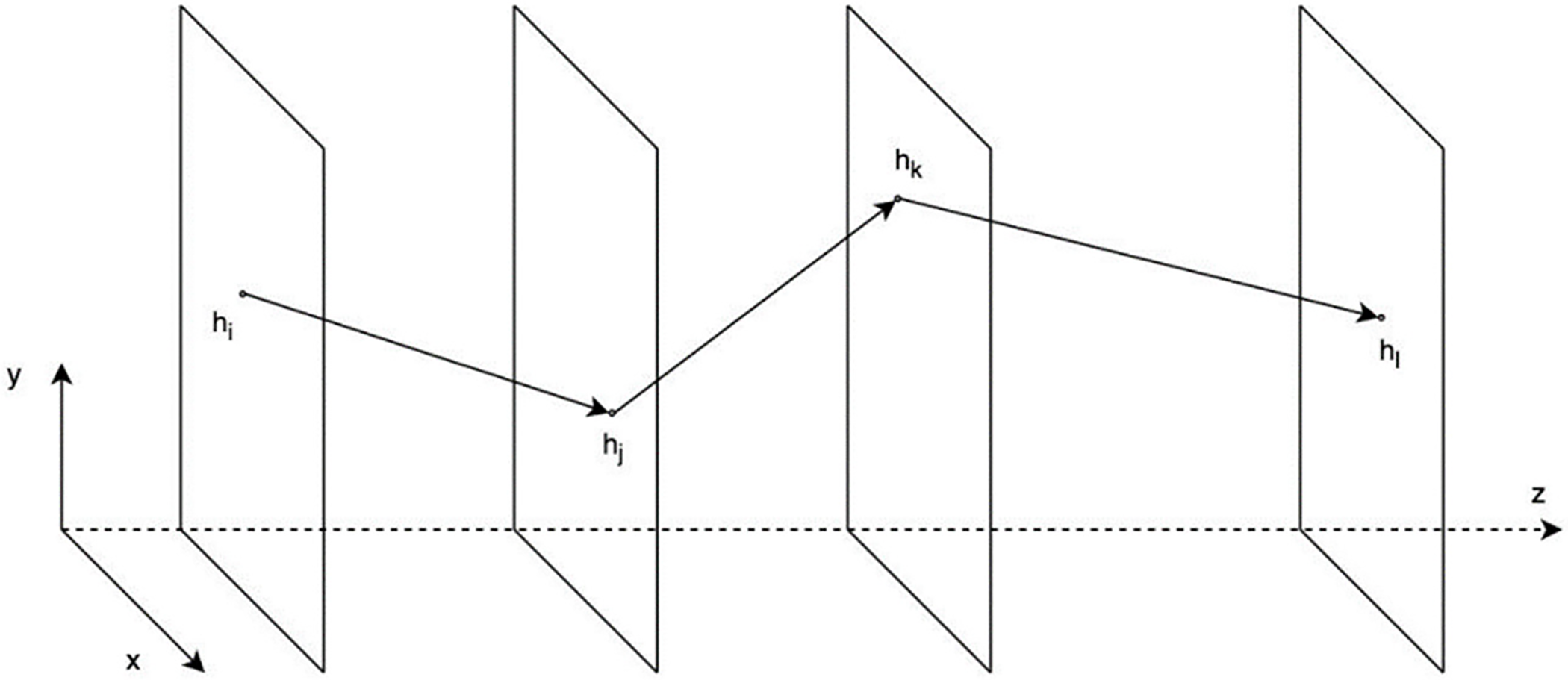
Figure 1: An example of a track t=[(hi,hj),(hj,hk),(hk,hl)]

As emphasized by Peterson [16], two factors must be considered when selecting segments for a track: the angle between two consecutive oriented segments (denoted as β) and the length sum of the two segments. Due to the high velocity of the particles and the influence of the magnetic field, their trajectories will either be slightly curved or follow almost straight lines. As a result, segments closer to the actual trajectory will have smaller β angles. The first objective, therefore, is to assess the difference between a straight line and the track. Fig. 2 illustrates two tracks—one in black and one in red—compared to an expected green trajectory. The red track has smaller β angles than the black track, indicating that it is closer to the actual trajectory.

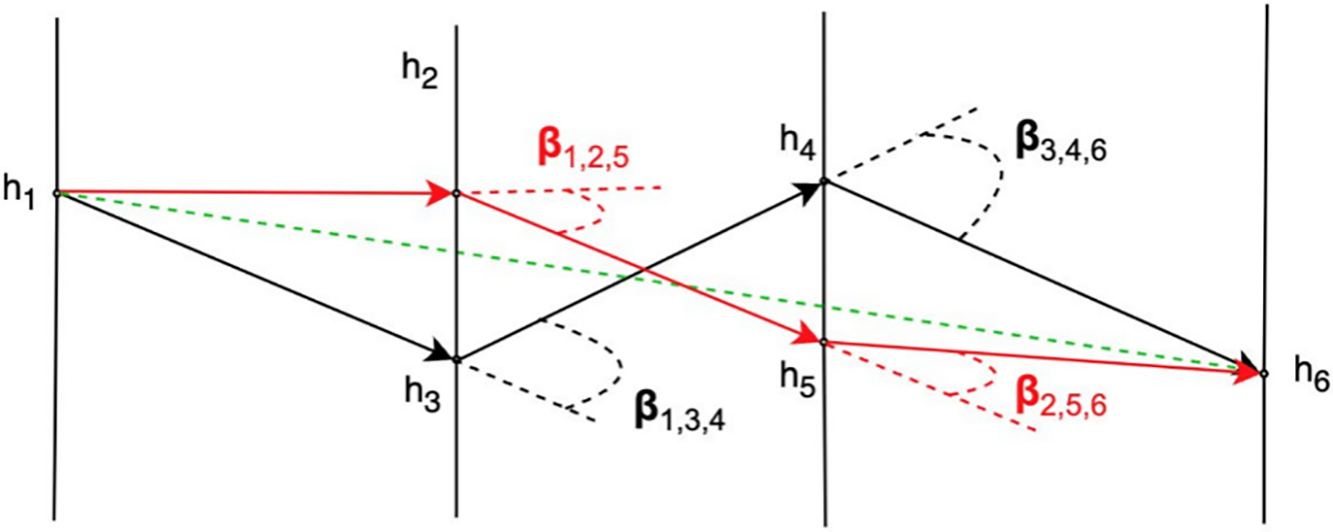
Figure 2: The first criterion of a quality track

The second objective is to choose between two tracks near the trajectory, with similar β angles, and to let the sum of the lengths of the segments be the deciding criterion. Consider the example in Fig. 3 showing two tracks, one in black with three adjacent segments and one in red with two adjacent segments.

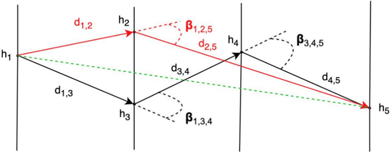
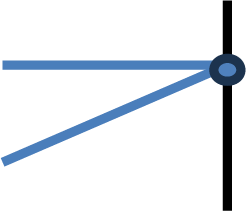
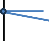
Figure 3: The second criterion of a good track

Let us suppose that cos⁡(β1,2,5)≈cos⁡(β1,3,4)+cos⁡(β3,4,5), call it θ, and that the length of the segments d1,2,d1,3,d3,4,d4,5 are approximately equal to 100 (arbitrary units), while d2,5 is approximately the double, 200. Then we have the Peterson [16] costs associated with the black track and the red track as follows:

cred=−cos⁡(β1,2,5)d1,2+d2,5=−θ300>cblack=−(cos⁡(β1,3,4)d1,3+d3,4+cos⁡(β3,4,5)d3,4+d4,5)=−θ200(1)

The cost associated with the black track is, therefore, lower than that of the red track, indicating that a track with more small consecutive segments is preferred.

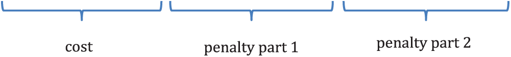
Hence, we have considered that the cost ci,j,k of two adjacent consecutive segments {(hi,hj),(hj,hk)} is determined by the angle βi,j,k and by the lengths of the two segments di,j,dj,k.

ci,j,k=−cos⁡(βi,j,k)di,j+dj,k(2)

as illustrated in Fig. 4. For small βi,j,k angles, when cos⁡(βi,j,k)≈1, this cost term will be negative and the total cost of a track candidate will be the solution of a minimization problem. Also, the combination of shorter segments will be privileged compared to longer ones, since their sum appears in the denominator.

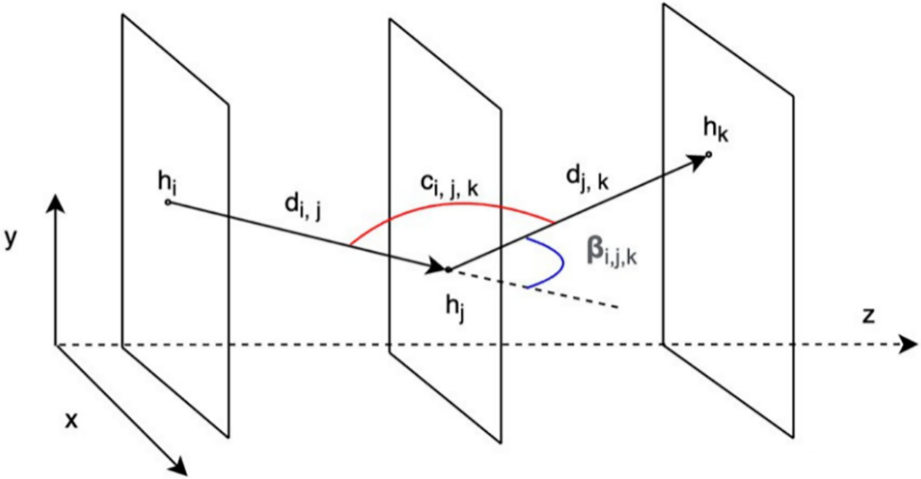
Figure 4: An example of the cost of a track

In our studies we have used the following notations to describe the data (list indexes start from 1):

•   L: the number of layers

•   HS: an ordered list of hits

•   N: the total number of hits

•   NL: the number of hits in layers 1 to L − 1 (excluding the last layer)

•   hi: hit number i in the list HS, with i=[1,N]

•   βi,j,k: the angle between two segments (hi,hj) and (hj,hk)

•   di,j: the length of segment (hi,hj)

•   ci,j,k: the associated cost if the segments (hi,hj) and (hj,hk) are in the same track, with ci,j,k=−cos⁡(βi,j,k)di,j+dj,k.

The variables used for modeling the problem are:

•   xi,j: a binary decision variable for segment (hi,hj) taking the values

xi,j={1,if the segment (hi,hj)is assigned to atrack0, otherwise.

2.2 Quadratic Constrained Binary Model—QCBM

We build the QCBM based on two parts: the objective function part and the constraints part.

The objective function part describes the objective which is to minimize the cost of all segments:

Min(α⋅∑ci,j,k⋅xi,j⋅xj,k),α>0(3)

The constraints part describes two conditions to build a track:

(1)   to any hit hj we receive exactly one segment unit from hit hi:

∑ixi,j=1,∀j         

(2)   for any hit hi we send exactly one segment unit to hit hj:

∑jxi,j=1,∀i         

with xi,j is binary ∀i,j.

This model can be solved either by using CPLEX or as a Constrained Quadratic Model (CQM) with a D-Wave hybrid solver. We will also use a Simulated Annealing library from D-Wave on a classical computer.

Therefore, the Hamiltonian of the problem will be:

H=−α⋅∑ci,j,k⋅xi,j⋅xj,k+γ⋅∑j(1−∑ixi,j)2+γ⋅∑i(1−∑jxi,j)2(4)

with the multipliers γ,α>0.

2.3 Binary Linear Program—BLP

Based on the QCBM, we transform the objective function into a linear form and introduce additional constraints to the previous ones, as follows. Consider the new variables zi,j,k=xi,j⋅xj,k which, together with the old ones, satisfy the constraints [7]:

•   xi,j+xj,k−zi,j,k≤1

•   zi,j,k≤xi,j

•   zi,j,k≤xj,k

•   0≤zi,j,k≤1

The objective is to minimize the cost of all segments:

Min(α⋅∑ci,j,k⋅zi,j,k),α>0(5)

with the following constraints, as before:

•   for any hit hj, we receive exactly one segment unit from hit hi:

∑ixi,j=1,∀j

•   for any hit hi, we send exactly one segment unit to hit hj:

∑jxi,j=1,∀i

•   xi,j is binary ∀i,j.

2.4 Models and Solvers

Starting with the three models introduced above and the three available solvers, we can study the six methods shown in Table 1.

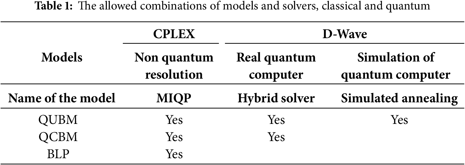
CPLEX can solve all three models, enabling us to treat optimization problems with either cost functions alone or with both cost functions and constraints. The hybrid solver, on the other hand, can only solve problems of the form Binary Quadratic Model (BQM) without constraints, Constrained Quadratic Model (CQM), or Quadratic Model (QM) without constraints. As a result, we use BQM for QUBM and CQM for QCBM. Simulated annealing can solve BQM, Quadratic Unconstrained Binary Optimization (QUBO), or the equivalent Ising models, so we will only do QUBM in this case.

3  The Set of Instances

A new set of instances is extracted from the Machine Learning training dataset of the TrackML Particle Tracking Kaggle Challenge [5]. Our goal is to study the scenario where the detection layers have all the same number of hits, equal to the number of particles traversing them (we call this a 100% detection efficiency). We follow two main steps to build this dataset:

•   Extract hits from the original dataset.

•   Preprocess the data (effectively build the instances).

In the first step, we extract the hit data from each detector layer in one compact volume of the detector, using data collected from 10 collision events of a total of 100 events available in the dataset. We then isolate the hits corresponding to the same particle, resulting in a dataset that will serve as the truth reference. Fig. 5 illustrates the parameters used to select the hits, including the number of hits per layer, the percentage of hits selected relative to the total hits per layer (100% in our first study), and the minimum momentum of the particle that generated the hits.

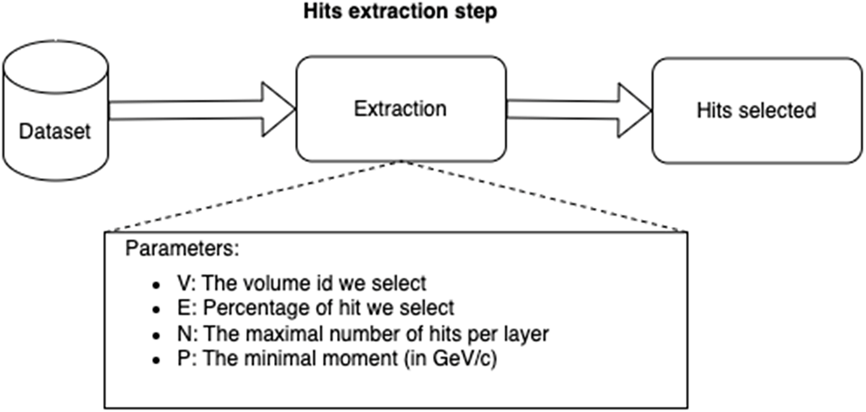
Figure 5: The hits extraction step

For example, when V = 9, N = 10, E = 100 and P = 1, it means we extract all hits from detector volume number 9, with 10 hits per layer, a selection ratio of 100%, and a minimum acceptable momentum of 1 GeV/c. The momentum is calculated and selected using the following formula:

pmin≤p=px2+py2+pz2(6)

where pmin is the minimum momentum, and px,py,pz are the momentum components (in GeV/c) along each coordinate axis. In the second step, we construct candidates for segments and we calculate possible segment pairs. A segment is considered valid if its direction remains within all detection layers, from the first to the last one, as shown in Fig. 6.

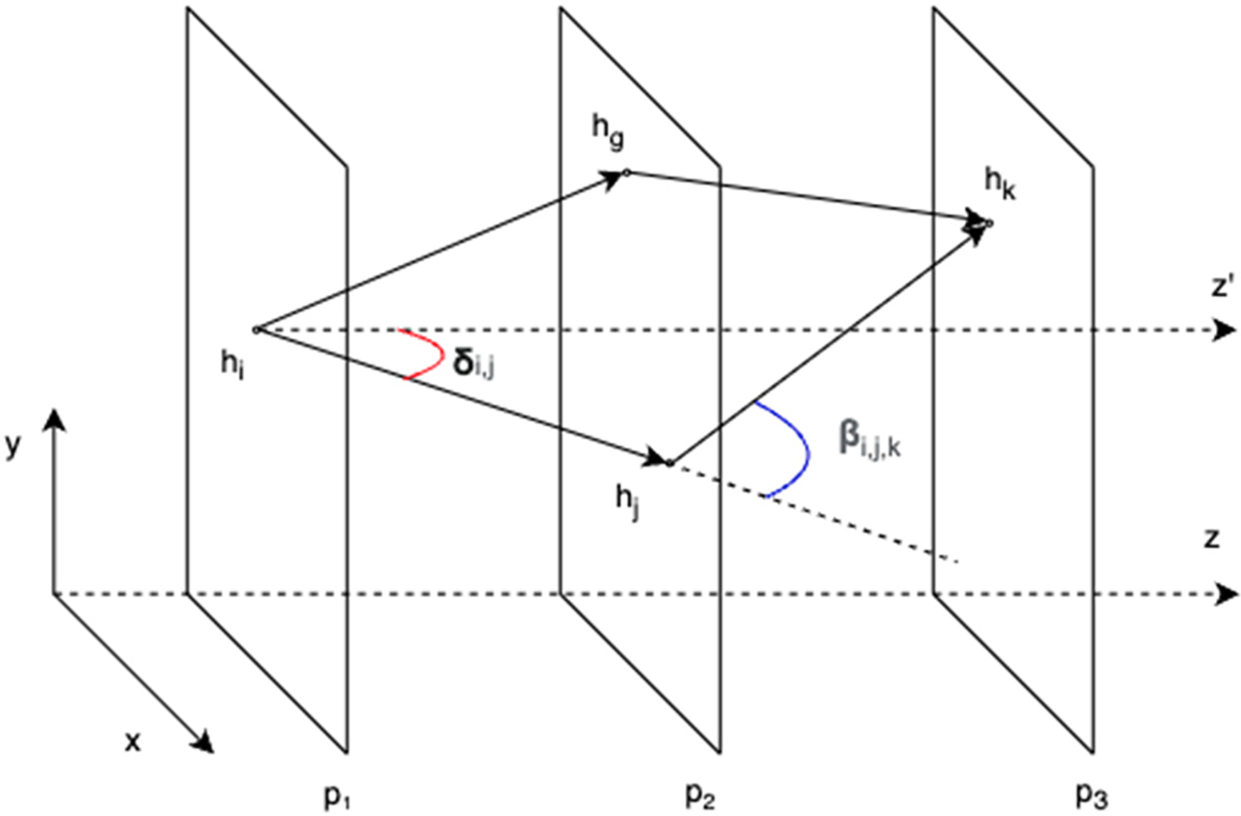
Figure 6: Build and filter segments

In order to reduce the number of generated segments from the N! possible combinations of N hits, we limit the angle between a segment and the z-axis. Additionally, a valid segment must have two hits detected by two consecutive detector layers, or at most two missing layers between them.

An instance is a set of hit tuples (hi,hj,hk) and their ci,j,k corresponding costs. This study uses the datasets described in Table 2, with the preprocessing time shown in Fig. 7. Details of each instance are described on our website1.

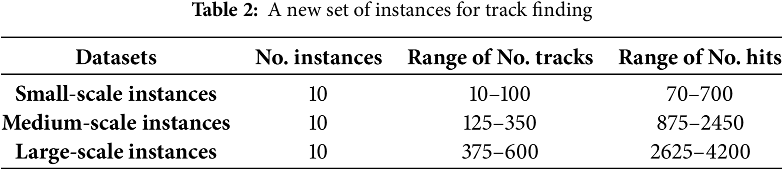
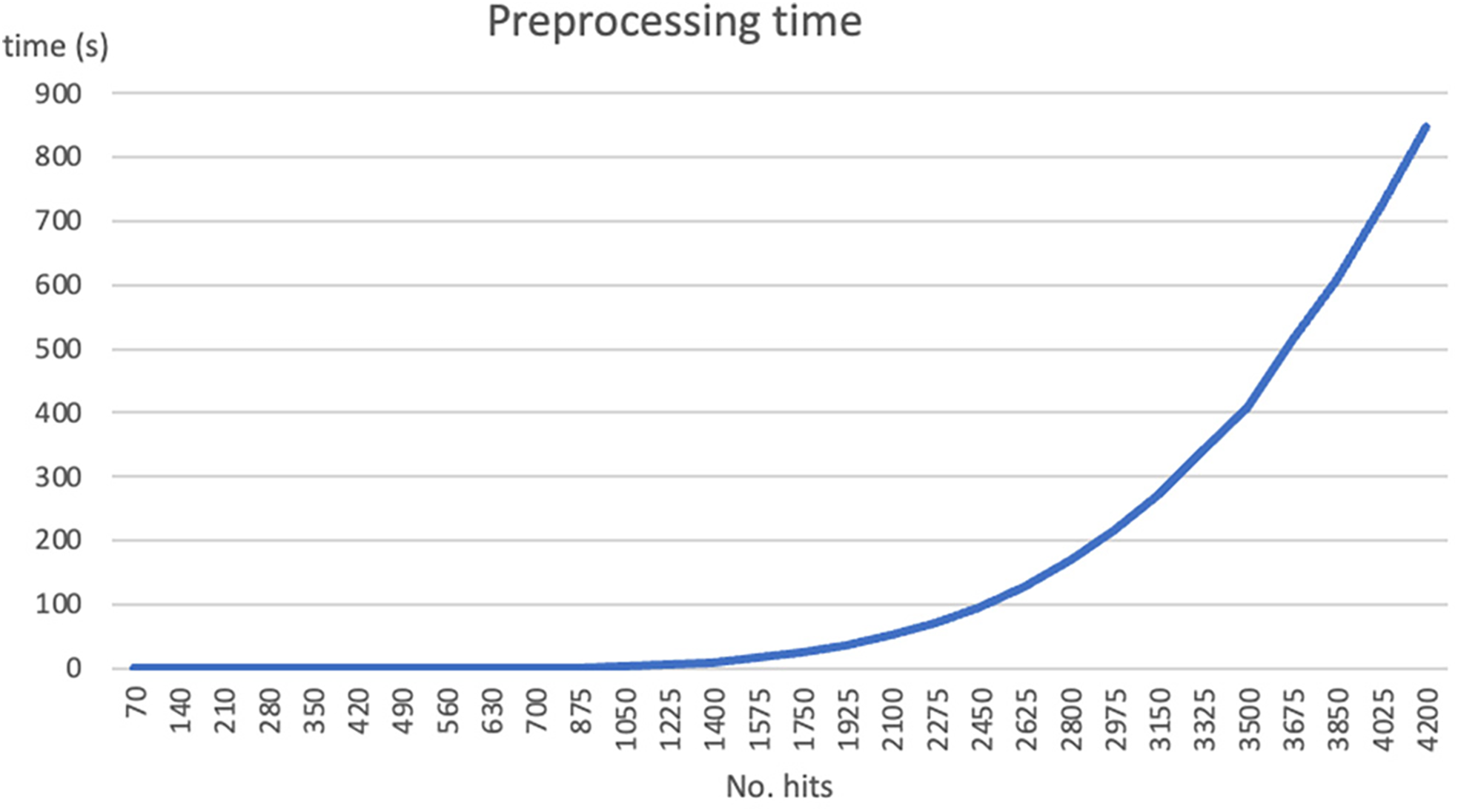
Figure 7: Preprocessing time of a new set of instances

The processing time for small datasets is almost negligible. However, for medium-scale to large-scale instances, the time increases rapidly, reaching up to 103 s.

The addition of preprocessing on the input data is based on the idea that the computation time spent on this step will be compensated by a significant reduction in the solving time, resulting in a substantial overall reduction in computation time, which must take into account both the preprocessing time and the time spent on solving. Depending on the problems, adding data filtering during the preprocessing phase results in a significant gain or not, depending on the specific issue.

4  Numerical Experiments

4.1 Evaluation

This study evaluates the track finding performance based on the gap ratio between the true cost and the computed cost as follows:

gap=100computedcost−truecosttruecost[%](7)

where

•   gap is the ratio error cost between the true cost and the computed cost,

•   truecost is the cost of tracks from the true hits information, and

•   computedcost is the cost of tracks the we compute by one of our methods.

4.2 Parameters

The experiments are based on 6 solutions methods including 3 solutions methods for the QUBM (Quadratic Unconstrained Binary Model), 2 methods for the QCBM (Quadratic Constrained Binary Model) and one method for the BLP (Binary Linear Program). To enhance readability, we name the solution methods as follows (see also Fig. 8).

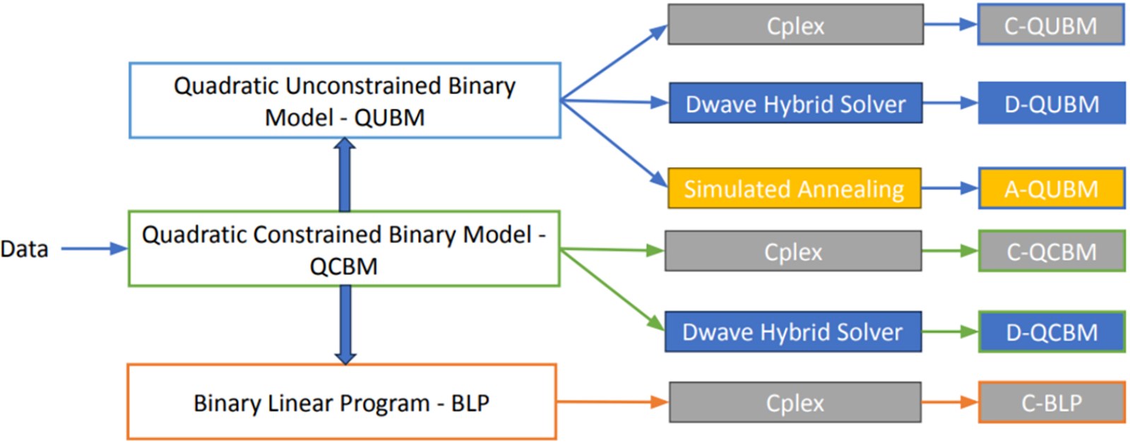
Figure 8: Classification of the methods. A_QUBM: solution of the QUBM (Quadratic Unconstrained Binary Model) using Simulated Annealing. C_BLP: solution of the BLP (Binary Linear Program) using CPLEX. C_QCBM: solution of the QCBM (Quadratic Constrained Binary Model) using CPLEX. C_QUBM: solution of the QUBM (Quadratic Unconstrained Binary Model) using CPLEX. D_QCBM: solution of the QCBM (Quadratic Constrained Binary Model) using D-Wave Hybrid Solver. D_QUBM: solution of the QUBM (Quadratic Unconstrained Binary Model) using D-Wave Hybrid Solver

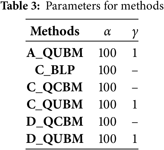
For this study we used the parameters shown in Table 3 for the 6 methods. All methods use α=100 because di,j is greater than or equal to 100(inµm units) and cos⁡(βi,j,k)≤1, therefore the cost will have a small value. The QUBM (Quadratic Unconstrained Binary Model) model will be better without α(α=1), because with small α the cost values form a fairly smooth landscape. This will make the time for finding the optimal solution longer. We use γ=1 such that the impact of the penalty functions is basically given by the number of segments.

4.3 Results

This section will compare the results according to different methods and datasets. For this, we will use the following notations:

•   S*: the optimal solution cost

•   S: the solution cost found by a method

•   PT: the preprocessing time (in seconds)

•   ST: the solution time (in seconds)

•   TT: the total time TT = PT + ST (in seconds)

•   GAP: the error percentage: GAP=100[(S−S∗)/S∗] (in %)

•   ATT: the average of the total time

•   AGAP: the average of the GAP

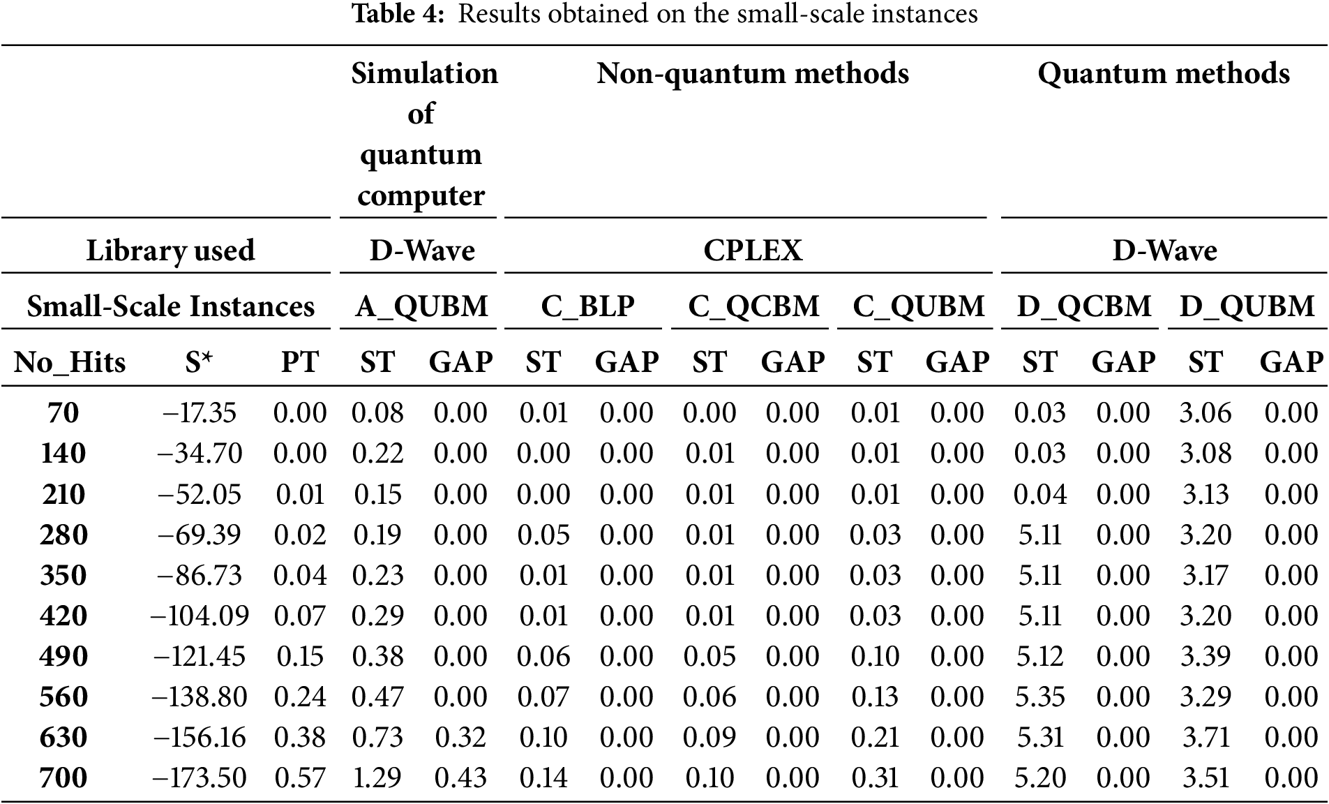
Table 4 demonstrates that the solution time for non-quantum methods is very short. In contrast, quantum methods take longer; however, their processing time remains consistent without significant increases. This suggests that, for a small number of hits, most methods provide both high accuracy and rapid processing time.

In Table 5, the solution time for most methods increases sharply, except for D_QCBM and A_QUBM, which stay under 10 s. For C_BLP and C_QCBM, we had to limit the time that CPLEX could use for solving the problem to 360 s, and for C_QUBM the time was again limited to 3600 s (excluding the time needed to create the Hamiltonian for CPLEX). While CPLEX delivers high accuracy, it comes at the cost of significantly increased solution time. For A_QUBM and D_QCBM, the solution time increases more slowly, but the optimality gap (GAP) rises rapidly, particularly in the case of A_QUBM. With D_QUBM, although the solution time increases, it does so at a manageable rate, and the GAP remains relatively stable. Therefore, for medium-sized datasets, D_QUBM demonstrates the effectiveness of the quantum method in balancing processing time and GAP ratio.

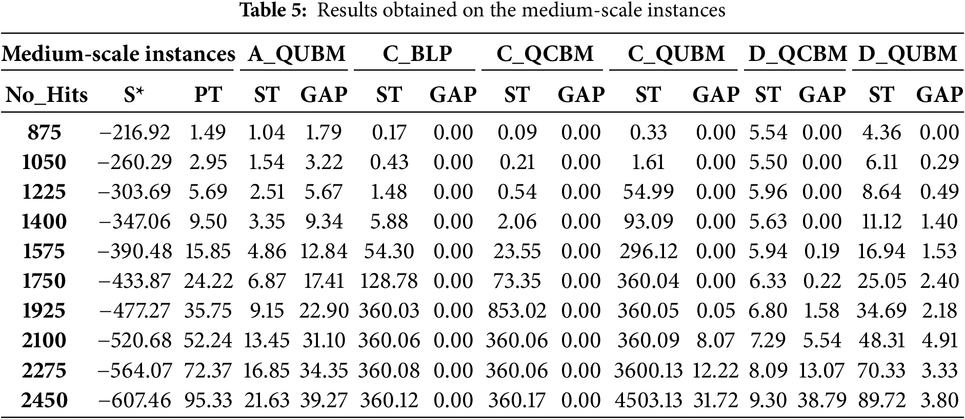
Table 6 contains many empty cells for the following reasons. For methods using CPLEX, the resolution time is excessively long to achieve a small GAP, making it impractical to obtain solutions within a reasonable processing time.

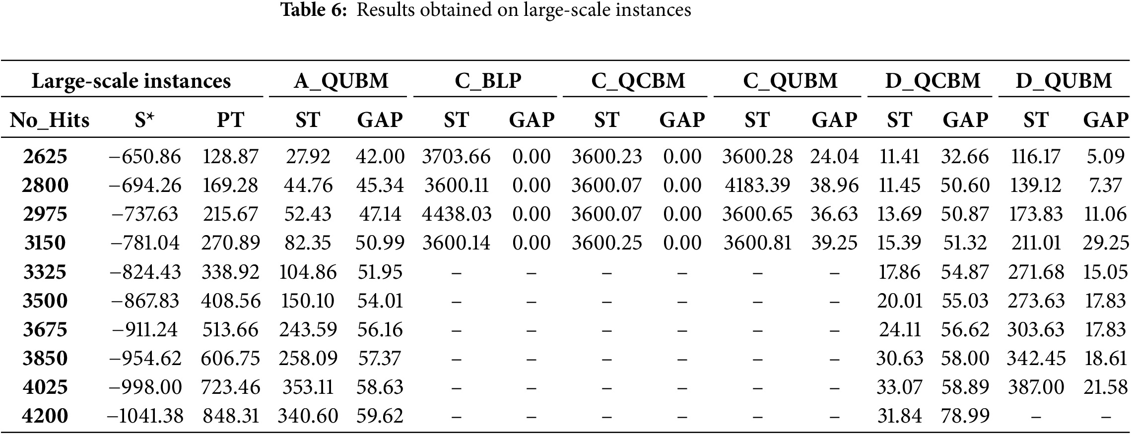
Therefore, the analysis focuses on A_QUBM and the two quantum methods The average results introduced in Table 7, gives a fair comparative study of methods. For A_QUBM, the resolution time does not increase rapidly, but the GAP remains consistently high. For the quantum methods, the D-Wave quantum computer imposes an overall running time limit of 20 min per month, in case of a free account. Despite this restriction, it was enough to solve the problem. With D_QCBM, the calculation time does not increase significantly because it uses a hybrid running mode, managing constraints on traditional computers while solving the cost function on quantum computers (Fig. 9). However, this approach sacrifices accuracy. In contrast, D_QUBM, while requiring more time for calculations, completes them within a reasonable time frame and delivers relatively good accuracy.

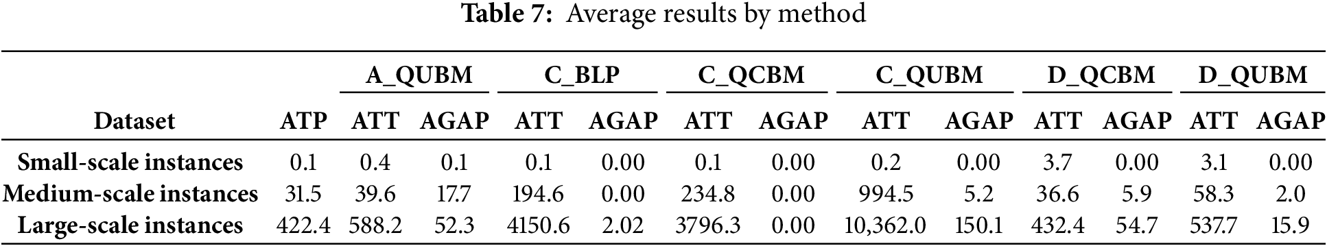
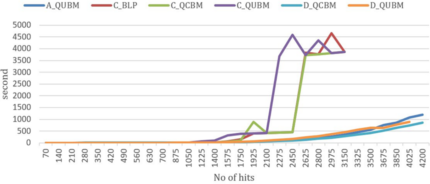
Figure 9: Total time from preprocessing to resolution of six methods

Fig. 10 illustrates the GAP ratio for six methods. Most methods using CPLEX exhibit small GAP values, except for C_QUBM, as this model lacks constraints and relies solely on a penalty function.

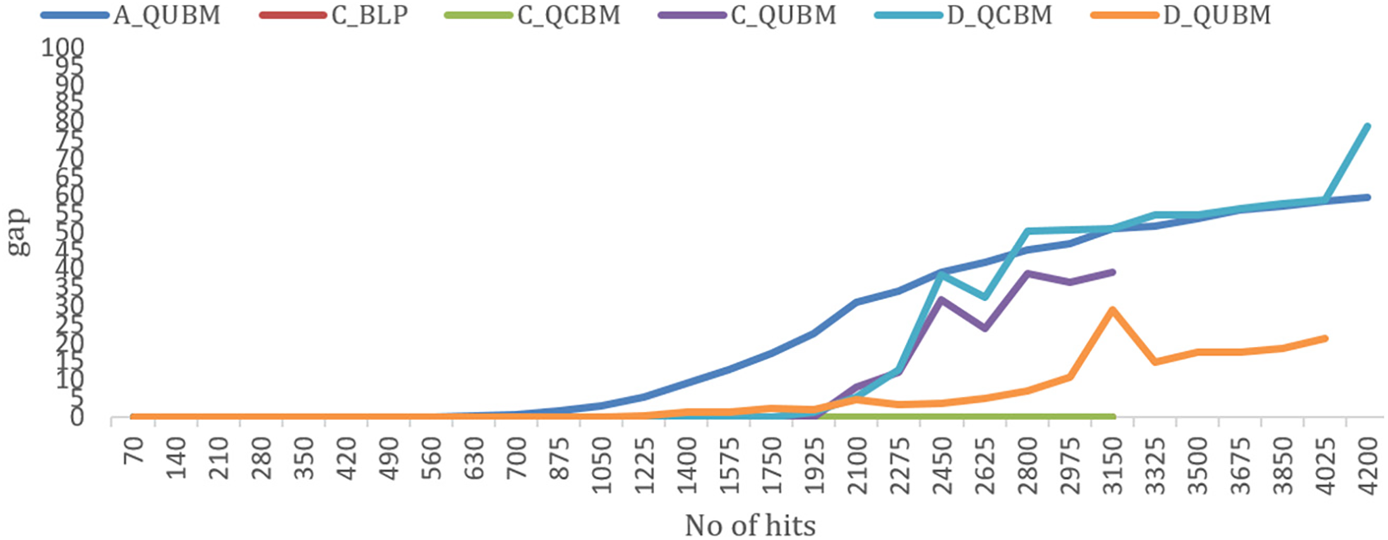
Figure 10: The GAP ratio for the six methods

When the number of hits increases, while the penalty term remains fixed at 1, the penalty function’s impact on the cost function diminishes. Some results of the track finding using simulated annealing (A-QUBM) running on a classical computer, for an increasing number of tracks, from 25-upper left to 150-bottom right are introduced in Fig. 11.

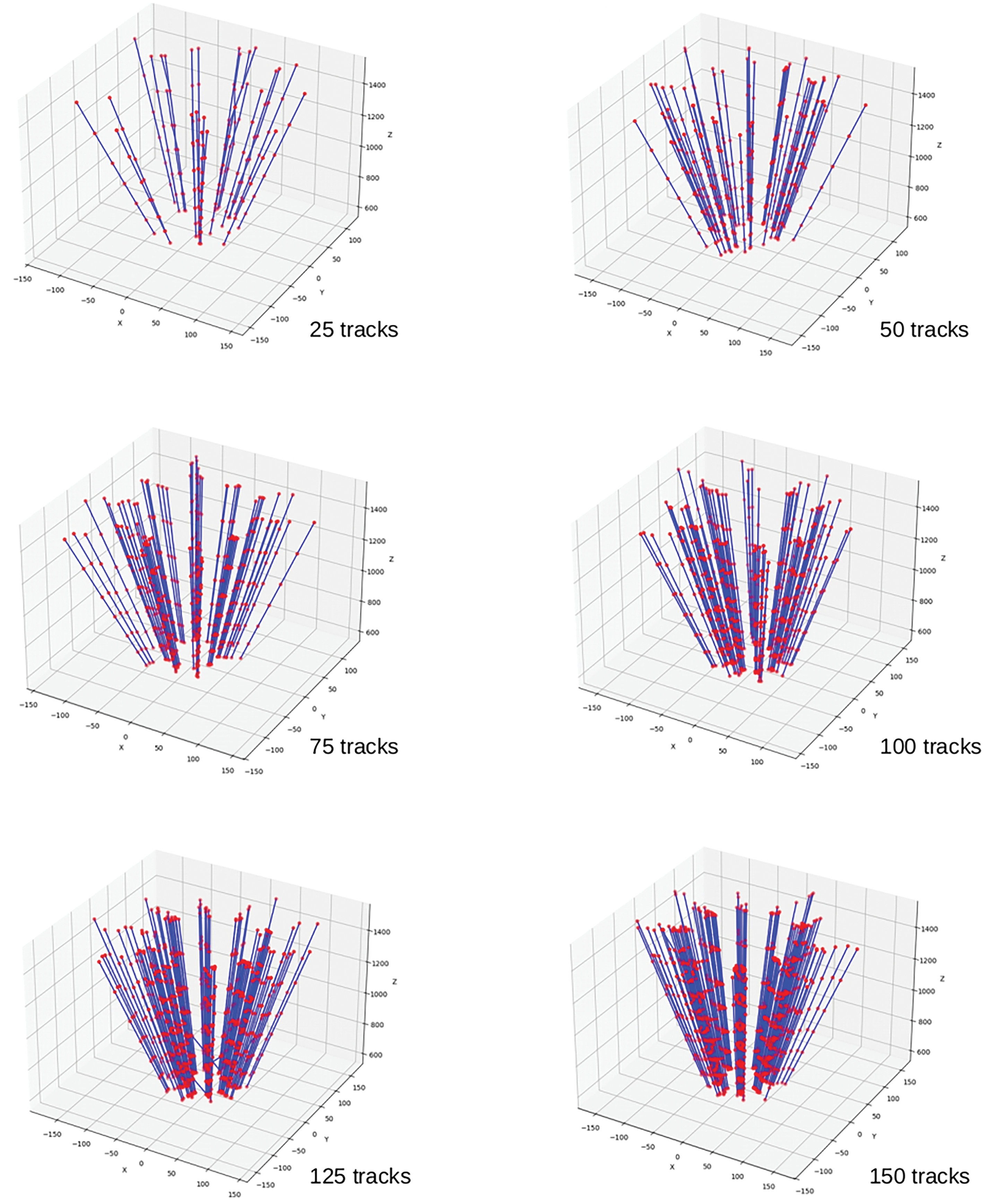
Figure 11: Some results of the track finding using simulated annealing (A-QUBM)

The corresponding number of hits is obtained by multiplying this number with the number of layers, 7. In the case of 25 tracks, no cut in the particle momentum was applied. For the other situations, a cut at 10 GeV/c was applied to the particle momentum. The tracks are all diverging from the collision point (not shown, somewhere below the horizontal xy plane) going upwards, and each track marks a hit on each of the seven layers, shown by the red points. The found segments, in blue, connect the hits in a single track, from the first to the last layer (ideally in the best case).

For A_QUBM, the GAP increases significantly and at an early stage. In contrast, D_QUBM performs much better, with a GAP of only about 22%. For D_QCBM, the initial performance is not better than A_QUBM, but as the number of hits increases, its GAP rises rapidly and eventually exceeds that of A_QUBM. These findings indicate that the QUBM model implemented on D-Wave delivers promising results. However, it is crucial to adjust the gamma parameter as the number of hits increases in order to maintain performance.

5  Conclusion

In this study, we developed and applied both classical and quantum computing technologies to address the track-finding problem, a highly challenging pattern recognition task in High Energy Physics, using QCBM, QUBM, and BLP models. All methods are designed to take a cloud of space points as input and assign labels such that points originating from the same particle share the same label. Our results show that achieving high accuracy with classical methods often requires substantial computation time. While Simulated Annealing on classical computers and the hybrid method for solving CQMs offer significantly faster solution times, their accuracy is notably lower. In contrast, solving the model using D_QUBM achieves high accuracy within an acceptable solution time. These findings highlight the promise of quantum computing as a future method for effectively solving this problem.

Acknowledgement: Thanks to the two anonymous reviewers who helped improve the article.

Funding Statement: The authors received no specific funding for this study.

Author Contributions: The authors confirm contribution to the paper as follows: study conception and design: Hervé Kerivin, Philippe Lacomme, Bogdan Vulpescu and Duy Dao; analysis and interpretation of results: Duy Dao and Bogdan Vulpescu; draft manuscript preparation: Philippe Lacomme, Bogdan Vulpescu and Hervé Kerivin. All authors reviewed the results and approved the final version of the manuscript.

Availability of Data and Materials: The data that support the findings of this study are openly available in: https://perso.isima.fr/~lacomme/track_finding/data.html (accessed on 1 January 2025).

Ethics Approval: Not applicable.

Conflicts of Interest: The authors declare no conflicts of interest to report regarding the present study.

1https://perso.isima.fr/~lacomme/track_finding/data.html (accessed on 1 January 2025).

References

1. Evans L. The large hadron collider. Annu Rev Nucl Part Sci. 2011;61(1):435–66. doi:10.1146/annurev-nucl-102010-130438. [Google Scholar] [CrossRef]

2. Ai X. Acts: a common tracking software. arXiv:1910.03128. 2019. [Google Scholar]

3. Apollinari G, Brüning O, Nakamoto T, Rossi L. High luminosity large hadron collider HL-LHC. arXiv:1705.08830. 2017. [Google Scholar]

4. Früwirth R, Strandlie A. Pattern recognition, tracking and vertex reconstruction in particle detectors. Berlin/Heidelberg, Germany: Springer; 2021. [cited 2025 Mar 10]. Available from: https://link.springer.com/book/10.1007/978-3-030-65771-0. [Google Scholar]

5. Calafiura P, Farrell S, Gray H, Vlimant JR, Innocente V, Salzburger A. TrackML: a high energy physics particle tracking challenge. In: IEEE 14th International Conference on e-Science; 2018 Oct 29–Nov 1; Amsterdam, The Netherlands. [cited 2025 Mar 10]. Available from: https://ieeexplore.ieee.org/document/8588707. [Google Scholar]

6. Brown C, Spannowsky Tapper A, Williams S, Xiotidis I. Quantum pathways for charged track finding in high-energy collisions. arXiv:2311.00766. 2023. [Google Scholar]

7. Group BI, Bertacchi V, Bilka T, Braun N, Casarosa G, Corona L, et al. Track finding at belle II. arXiv:2003.12466v2. 2021. [Google Scholar]

8. Qu Z, Haino S, Zuccon P, Zhao M. New track finding based on cellar automaton for AMS-02 detector. Nucl Instrum Methods Phys Res Sect A Accel Spectrometers Detect Assoc Equip. 2024;869:135–40. doi:10.1016/j.nima.2017.07.007. [Google Scholar] [CrossRef]

9. Kucharczylk M, Wolter M. Track finding with deep neural networks. Comput Sci. 2019;20(4):475–91. [Google Scholar]

10. Gessinger-Befurt P. Development and improvement of track reconstruction software and search for disappearing tracks with the ATLAS experiment [dissertation]. Mainz, Germany: Gutenberg-Universitätin Mainz; 2021. [cited 2025 Mar 10]. Available from: https://cds.cern.ch/record/2771309. [Google Scholar]

11. Schut M. Track finding in physics a review of existing methods and an exploration of two new methods [master’s thesis]. Groningen, The Netherlands: Univeristy of Groningen; 2017. [cited 2025 Mar 10]. Available from: https://fse.studenttheses.ub.rug.nl/id/eprint/15324. [Google Scholar]

12. Rajak A, Suzuki S, Dutta A, Chakrabarti BK. Quantum annealing: an overview. Phil Trans R Soc A. 2023;381:20210417. doi:10.1098/rsta.2021.0417. [Google Scholar] [PubMed] [CrossRef]

13. Vaezi A, Movaghar A, Ghodsi M, Kaemi SMH, Noghrehy NB, Kazemi SM. Quantum computational complexity vs. classical complexity: a statistical comprehensive analysis of unsolved problems and identification of key challenges. arXiv:2312.14075v5. 2024. [Google Scholar]

14. Kikuura S, Igata R, Shingu Y, Watabe S. Performance benchmarking of quantum algorithms for hard combinatorial optimization problems: a comparative study of non-FTQC approaches. arXiv:2410.22810v1. 2024. [Google Scholar]

15. Liu Q. Comparisons of conventional computing and quantum computing approaches. Highlights Sci Eng Technol. 2023;38:502–7. doi:10.54097/hset.v38i.5875. [Google Scholar] [CrossRef]

16. Blume-Kohout R, Young K. Quantum computing metrics and benchmarking frameworks: not yet. In: The International Conference on Rebooting Computing Workshop on Quantum Metrics & Benchmarks; 2018 Nov 7–9; Washington, DC, USA. [cited 2025 Mar 10]. Available from: https://www.osti.gov/biblio/1594677. [Google Scholar]

17. Acuaviva A, Aguirre D, Pena R, Sanz1 M. Benchmarking quantum computers: towards a standard performance evaluation approach. arXiv:2407.10941v2. 2024. [Google Scholar]

18. King AD, Nocera A, Rams MM, Dziarmaga J, Wiersema R, Bernoudy W, et al. Beyond-classical computation in quantum simulation. Science. 2025;388(6743):199–204. doi:10.1126/science.ado6285. [Google Scholar] [PubMed] [CrossRef]

19. Peterson C. Track finding with neural networks. Nucl Instr Meth A. 1989;279(3):537–45. doi:10.1016/0168-9002(89)91300-4. [Google Scholar] [CrossRef]