Research on Plant Species Identification Based on Improved Convolutional Neural Network

1  Introduction

It is well known that the diversity of plant species plays a very important role in various fields, such as agriculture, industry, medicine, environmental protection, human daily life and production activities, etc. Plants provide a large amount of food and some necessities and maintain the balance of carbon dioxide and oxygen in the atmosphere. In addition, plants are also important in concealing water, preventing desertification, and improving climate. However, in recent years, with the increase in human production activities and rapid urban development, as well as over-cultivation, global warming, severe environmental pollution, and insufficient knowledge of plant species, human beings have not only destroyed the living environment but also the biological ecology, leading to the extinction of hundreds of plant species [1]. Pimm et al. [2] mentioned that about 150,000 plant species in the world are on the verge of extinction, accounting for one-third of the world’s 450,000 known plant species and that environmental degradation will lead to the extinction of 27%–33% of the planet’s species by the end of the 21st century. Therefore, the conservation of plant diversity is an important and urgent task. The first step in conserving plant species is to recognize them and understand what they are and where they come from [3]. However, it is a challenge for human beings to accurately identify these plant species, as plant species identification requires specialized botanical knowledge and in-depth systematic training [4]. Identifying a large number of extant plant species is very time-consuming and almost impossible, especially for non-experts. Therefore, there is a need for taxonomic studies of plant species, and plant species identification facilitates the development of an understanding of plant species and provides guidance and comprehensive learning for beginners in the field to better conserve and value plant species.

With the development of computer hardware and software, mobile devices, image processing, and machine learning [5–9], it is feasible and meaningful to design a fast and efficient method to automatically identify and classify plant species. Plant species can be classified and identified by different organs such as leaves, flowers, fruits, or whole plants [10–12]. Much information about plant species identification is stored in the leaves of plants. However, leaves exist on plants for only a few months a year, while flowers and fruits may exist for only a few weeks. This is the main reason why many plant species identification tools are based on leaf image databases. Compared to other organs, leaves are more stable in shape and structure and are largely planar, making them suitable for two-dimensional image processing. Therefore, plant species can be identified by the shape, color, and texture of leaves, but leaf color characteristics are rarely used to identify plant species because leaf color is variable across seasons and in the surrounding environment [4]. The diversity of leaf morphology is an important basis for plant taxonomic identification [13,14]. Leaf texture characteristics are mainly the characteristic information contained in the leaf vein sequence, which can describe the internal structure of the whole leaf. The structure of leaf venation within species is relatively stable, and the structure of leaf venation varies widely among species. In general, the leaves of each plant have many invariable features, such as shape, texture, tip, and base, that can be used to identify and classify species [3]. Therefore, most of the existing species identification methods are based on the shape and texture of leaf images and have been proven reliable over the years. Wang et al. [15] proposed a chord bundle walk (CBW) shape descriptor for plant leaf identification and obtained good retrieval results on a large-scale plant leaf dataset. Alamoudi et al. [16] proposed a plant leaf recognition method using texture features and semi-supervised spherical k-means clustering, which reduces the need for large-scale labeled data and extends the application of the method. However, the method only considers the texture features of leaves and has low recognition performance. Zhao et al. [17] proposed a count-based shape representation method that accurately identifies simple and composite plant leaves with high recognition efficiency. Metre et al. [18] provided a brief overview of different aspects of plant leaf classification in recent years and discussed the different ways of elaborating on the plant leaf classification problem in many pieces of literature ways. In contrast to the study of plant leaves, species can also be identified based on flowers. Some studies have focused not only on the overall region of the flower but also on some parts of the flower. Yuan et al. [19] proposed a framework for phenotype classification of chrysanthemum images based on transfer learning and bilinear convolutional neural networks. A symmetric VGG16 network was used as the feature extractor. The pre-trained parameters were then transferred to the proposed framework, which was divided into two stages for training the fully connected layer and fine-tuning all layers, respectively. The phenotypic features of chrysanthemum yield in these two networks are transposed and multiplied. Finally, the global features are fed into the classification layer for classification. The experimental results show that this scheme can obtain better performance and lower loss with an accuracy of 0.9815 and a recall of 0.9800 compared to other network models. Guru et al. [20] studied the effect of texture features on flower image classification by extracting texture features, that is, color texture, grayscale covariance matrix, and Gabor response, and using a combination of all three in flower classification. Lee et al. [21] proposed a multilayer technique based on the natural environment of flower species for the identification and retrieval of flower species in natural environments. The optimal method for color, texture, and shape feature extraction was experimentally analyzed, and the results showed that it was most effective to fuse the color, texture, and shape features of the flower images.

Traditional methods for plant species recognition have several drawbacks: features need to be manually designed and cannot be automatically learned, and vision-based features often cannot be taken into account simultaneously, thus reducing recognition accuracy [22,23]. Compared with traditional methods, deep learning can solve the above problems. Deep learning is a set of algorithms in machine learning [24] that can automatically learn high-level robust representations of plant images and discover more effective discriminative features than those used for plant recognition in previous studies [25]. Compared to classical machine learning algorithms, deep learning methods are more suitable for processing high-dimensional data. Through its wide range of computational power, deep learning has proven to be a very powerful approach in various applications [24]. Many deep learning models, such as convolutional neural networks (CNN), deep belief networks (DBN), and recurrent neural networks (RNN), have been applied to various fields, including image classification, signal and language processing, computer vision, speech recognition, drug design, material detection, and plant species recognition, with state-of-the-art results, sometimes exceeding human-level capabilities [26,27]. In particular, CNN is one of the most popular deep-learning paradigms. Two main advantages of CNN are local connectivity and weight sharing in the convolutional layers (https://en.wikipedia.org/wiki/Convolutional), making them closer to biological neural networks and reducing the complexity of network models and weights. Unlike traditional image recognition methods, it can directly input the original 2D image into the network to automatically extract salient features, avoiding the complex image pre-processing, manual feature extraction, and data reconstruction processes in classical recognition algorithms. Therefore, it has become a research hotspot in various fields, especially in image recognition. Zhang et al. [1] briefly introduced the existing plant species identification methods and summarized each method’s advantages and disadvantages. Patil et al. [28] performed a comparative analysis of various methods for plant identification, and experiments conducted in Swedish leaves verified the effectiveness of machine learning and CNN-based classification models. Wäldchen et al. [29] synthesized and compared the preliminary studies of computer vision methods in plant species identification. They analyzed in detail more than 120 peer-reviewed research results published in the last 10 years (2005–2015) and classified them according to the plant organs and characteristics studied, such as shape, texture, color, margin, and leaf vein structure. In addition, they compared the methods of classification accuracy achieved on several publicly available datasets.

The improved method based on the ShuffleNetV2 convolutional neural network proposed in this study achieved better results in plant image recognition compared to the traditional methods. Six convolutional neural network models were designed, containing enough trainable parameters to learn discriminative features, and the training process was optimized using the stochastic gradient descent (SGD) algorithm to avoid overfitting or falling into local optima [30]. The SGD algorithm is a very common, simple, and effective optimization algorithm in neural network model training. This algorithm is generated based on the gradient descent algorithm and is mostly used for learning linear classifiers under convex loss functions such as support vector machines (SVM) and logistic regression [31]. And SGD has been successfully applied to large-scale and sparse machine learning problems frequently encountered in text classification and natural language processing. SGD can be used not only for classification computations but also for regression computations. Mutlu et al. [32] proposed a parallel hybrid algorithm combining SVM, sequential minimum optimization (SMO), and SGD methods to optimize the weight cost of computation. The performance of the proposed SVM-SMO-SGD algorithm was compared with the classical SMO and Computational Unified Device Architecture (CUDA) based approaches on well-known datasets (i.e., diabetes, medical stroke prediction, adults) and it was shown that the sequential SVM-SMO-SGD is 3.81 times faster in time and 1.04 times more efficient in RAM consumption than the classical SMO algorithm. On the other hand, the parallel SVM-SMO-SGD algorithm is 75.47 times faster in time than the classical SMO algorithm. It also consumes RAM 1.9 times more efficiently. The overall classification accuracy of all algorithms was 87% in the diabetes dataset, 95% in the healthcare stroke prediction dataset, and 82% in the adult dataset. Ren et al. [33] proposed a data-driven modeling approach for aero-engine aerodynamic models combining stochastic gradient descent with support vector regression. The modeling method was validated using simulation data from an aero-engine component-level model and flight data from a type of aircraft, and it provided better performance compared with the traditional method.

There are two main novelties in this research. First, the lightweight model ShuffleNetV2 1.0X is chosen as the baseline version, which has the advantage of considering the MAC (Memory Access Cost) at the beginning of the design, enabling a very low latency when deployed on mobile. In this study, we make some optimizations to improve the accuracy and reduce the computation, design six models with better structure than the baseline version, and test them on the constructed TJAU10 dataset to verify their better generalization performance. Second, this paper is not only the optimization of the simple convolutional neural network model but also a special feature to use the features of the whole plant (stem, leaf, flower, fruit, etc.) for plant species recognition. The advantage is that the deep learning algorithm based on the convolutional neural network can learn the plant image features independently, reduce human intervention, and improve the image recognition rate by excluding noise interference for natural background plant images. The existing plant species recognition methods have low recognition accuracy, and the recognition accuracy cannot meet professional needs. The purpose of this paper is to use the convolutional neural network model to recognize plant species based on the overall plant image characteristics by autonomously learning plant image features and reducing human intervention, and further improving the plant species recognition precision through model optimization. Finally, the model with the best performance was selected to meet the requirements of professionals for the accurate identification of plant species.

2  Material and Methods

2.1 Dataset

2.1.1 Data Collection

In November 2021, nearly 3,000 images of 10 plant species in the natural background were collected by cell phones on the campus of Tianjin Agricultural University to construct the Tianjin Agricultural University 10 dataset (hereinafter referred to as TJAU10). 4,000 × 3,000 pixels of cell phones were used to ensure that the collected data had a certain complexity, and different lighting and different shooting angles were used for the acquisition method. To facilitate the experiment, 10 plants were numbered from 1 to 10, and each number corresponds to the plant name as shown in Table 1. 2,134 plant images were finally screened and divided into a training set, validation set, and test set, and the ratio of both validation set and test set was 20%, which was about 400 images. 10 plant images are shown in Fig. 1, and the distribution of the number of each plant image is shown in Fig. 2.

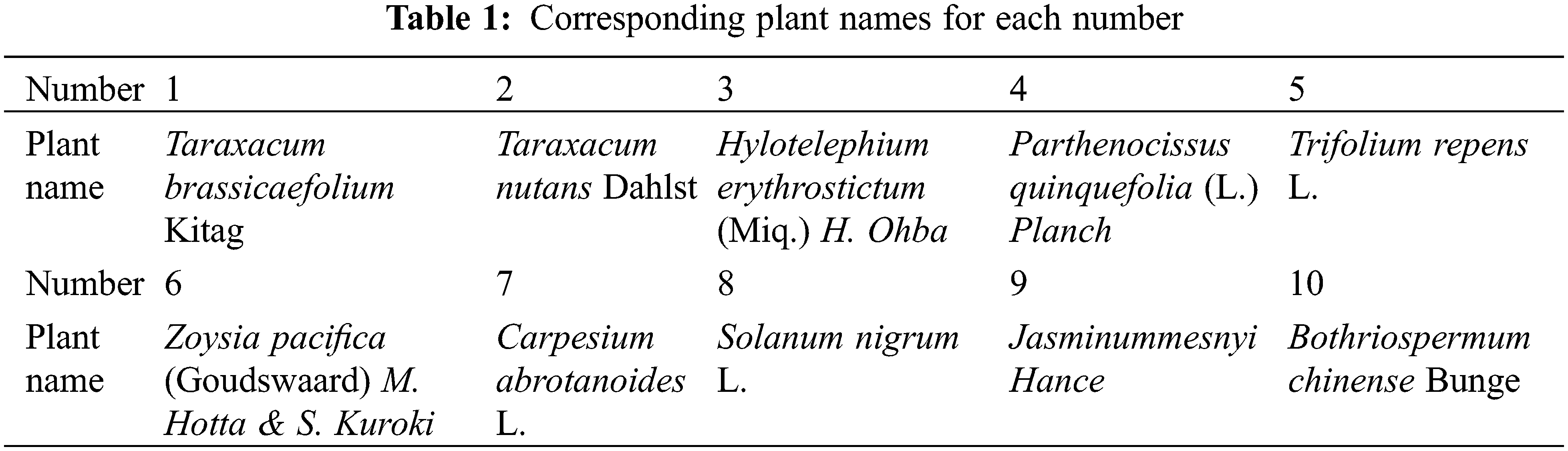
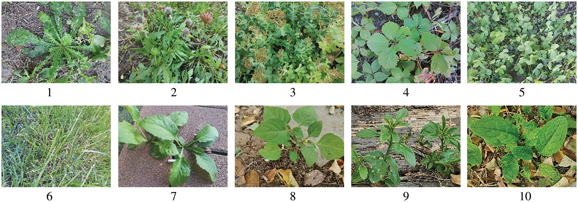
Figure 1: Images of 10 plant species

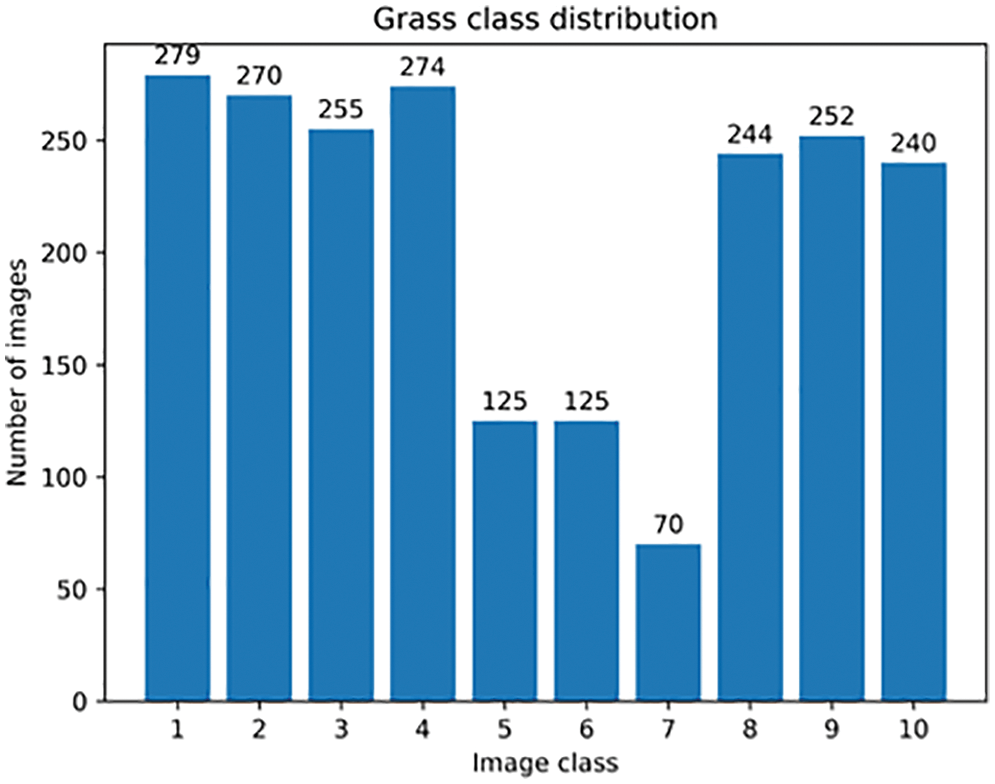
Figure 2: Distribution of the number of each plant image

2.1.2 Data Preprocessing

The purpose of data preprocessing is to enhance image data, reduce distorted data and features, and enhance image features relevant to further processing. The preprocessing subprocess receives an image as an input and generates a modified image as an output for the next step of feature extraction. Preprocessing operations usually include image noise reduction [34], random cropping, horizontal or vertical flipping, image brightness adjustment [35], etc. These methods can be applied in parallel or individually, or multiple times until the image quality meets the experimental requirements [36]. In this paper, the dataset was taken by cell phones, and the plant images were noisy, but using traditional filtering methods would increase the computational effort substantially and also cause the loss of some features, so no image denoising was done in this paper. To expand the data, the images are randomly cropped to 224 × 224 pixels. To enhance the robustness of the model, a horizontal flip operation is performed on the images. To speed up the convergence, the pixel points of the plant images are normalized. The plant image with the number 9 and the name Jasminummesnyi Hance is used as an example to demonstrate the image changes before and after data preprocessing, as shown in Fig. 3.

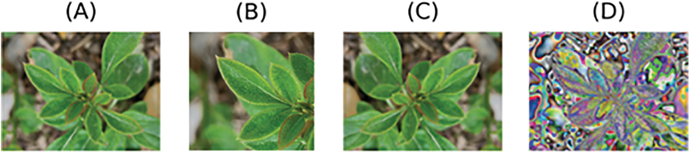
Figure 3: Image changes before and after data preprocessing. (A) original image; (B) random cropping of the image to 224 × 224 pixels; (C) random horizontal flipping operation of the image; (D) normalization of the pixel points of the image

2.2 Model Architecture

In the mobile scenario, there are many good lightweight networks to choose from, such as Google’s MobileNet series, Kuangsi’s ShuffleNet series, Huawei’s GhostNet, etc. Among these models, ShuffleNetV2 is widely used because of its clear and concise structure [37], as shown in Fig. 4 for ShuffleNetV2 1.0X, which is designed with MAC in mind at the beginning of the design, enabling a very low latency when deploying on mobile. Tests on the constructed dataset also validate its better generalization performance. However, sometimes some optimization of ShuffleNet is still needed to realize the use of ShuffleNet in embedded scenarios with lower computational resources or to use ShuffleNet as a backbone in lightweight detection frameworks. In this paper, we design a better model structure than the baseline version by improving ShuffleNetV2 version 1.0X, including two dimensions of improved accuracy and reduced computation.

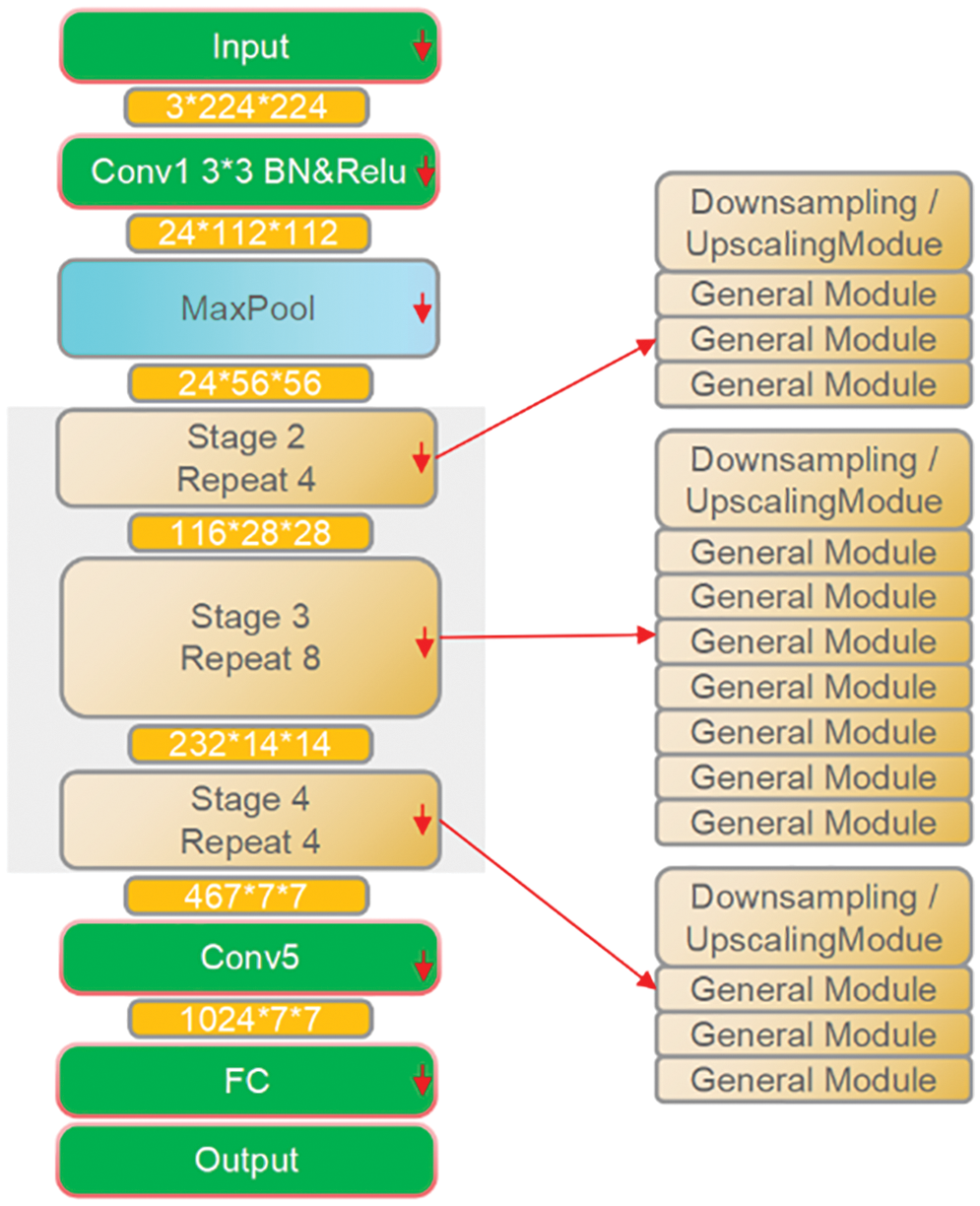
Figure 4: Architecture diagram of ShuffleNetV2 1.0X

2.2.1 Improving Accuracy

To improve the accuracy, we combine ShuffleNetV2 with SENet and SKNet attention mechanisms to obtain ShuffleNet_SE and ShuffleNet_SK networks, respectively. By adjusting the size of the depth-separable convolutional kernel in the downsampling of ShuffleNetV2, we obtain the ShuffleNet_K5 network by expanding all 3 * 3 depthwise convolutions in the downsampling to 5 * 5. The ShuffleNet_Ks4 network is obtained by expanding the depthwise convolution of 3 * 3 in the downsampled single branch to 4 * 4.

ShuffleNet_SE Network

Mainly, we borrow the channel attention mechanism in SENet [38] and apply it to ShuffleNetV2 to get the ShuffleNet_SE network, whose module structure is shown in Fig. 5.

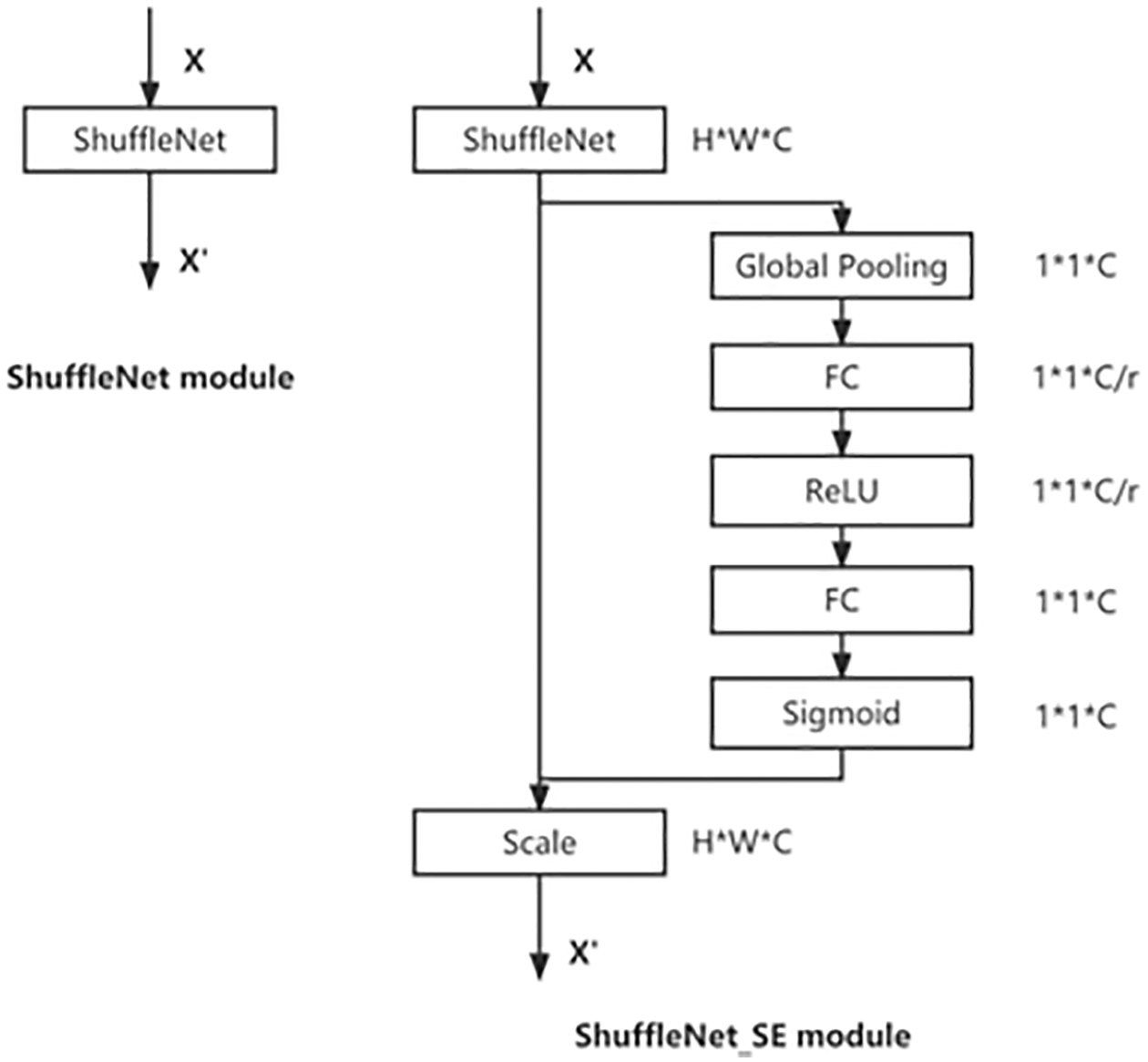
Figure 5: The schema of the original ShuffleNet module (left) and the ShuffleNet_SE module (right)

For each input X, there are two main operations: squeeze and excitation. Squeeze refers to compressing the spatial information of features by global average pooling, which compresses the original C * H * W dimensional information to C * 1 * 1. Excitation uses two fully connected layers, the first one reduces the dimensionality and downscales C * 1 * 1 to C/r * 1 * 1 (with ReLU activation), and the second FC layer maps the features back to C * 1 * 1 (without ReLU activation), and then after sigmoid, the weight coefficients of each channel are obtained. Then the weight coefficients are multiplied with the original output channel features of each channel to get a new weighted feature, called feature recalibration.

ShuffleNet_SK Network

We mainly borrowed from the attention mechanism in SKNet [39] for selecting the output of large or small convolutional kernels. The principle is shown in Fig. 6.

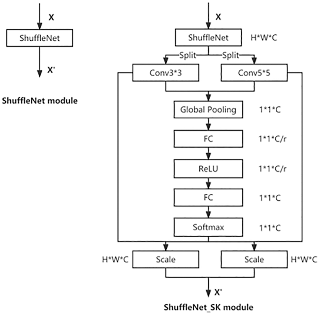
Figure 6: The schema of the original ShuffleNet module (left) and the ShuffleNet_SK module (right)

The new features U3 * 3 and U5 * 5 are obtained by passing feature X through the small convolution kernel (3 * 3) and the large convolution kernel (5 * 5), respectively. Then the two new features U are summed, and the weight vectors are obtained after the same squeeze and excitation as SENet. Finally, the weight vectors are multiplied with the corresponding U respectively and then summed to get the new features.

ShuffleNet_K5 Network

Looking at the distribution of the computation of ShuffleNetV2, the computation on the depthwise convolution is very small, and the main computation is on the 1 * 1 convolution. ShuffleNet_K5 replaces all the 3 * 3 depthwise convolutions with 5 * 5 depthwise convolutions. In the PyTorch implementation, the padding needs to be modified from 1 to 2, so that the output feature map can maintain the same resolution as the original. The principle is shown in Fig. 7.

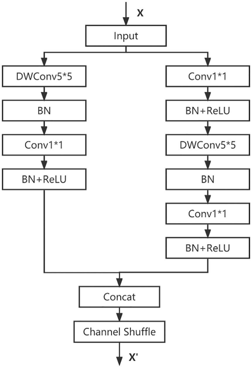
Figure 7: ShuffleNet_K5 network structure

ShuffleNet_Ks4 Network

ShuffleNet_Ks4 replaces the single branch 3 * 3 depthwise convolution with a 4 * 4 depthwise convolution in the downsampling, and in the PyTorch implementation, the padding size is set to 1 to ensure consistent input and output resolution of the feature map. The principle is shown in Fig. 8.

Figure 8: ShuffleNet_Ks4 network structure

2.2.2 Reducing Computational Effort

To reduce the computational effort, we optimized ShuffleNetV2 using convolutional cropping and CSP techniques, respectively. The insignificant 1 * 1 convolution in the ShuffleNetV2 block is cropped to obtain the ShuffleNet_LiteConv network. The network is reorganized using the CSP technique to obtain the ShuffleNet_CSP network.

ShuffleNet_LiteConv Network

By observing the blocks of ShuffleNetV2, it can be divided into two structures. One is the first block of each stage, which copies the input into two portions, extracting features by convolution of branch1 and branch2 respectively, and then concatenating together, as shown in Fig. 9A. Another common block splits the input into branch1 and branch2, and branch1 is directly concatenated with the part of branch2 that has been extracted by convolutional features, as shown in Fig. 9B.

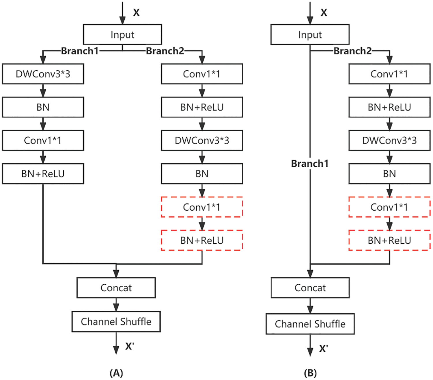
Figure 9: Block structure of ShuffleNet. (A) Downsampling Block; (B) General Block

Generally, 1 * 1 convolution is used before or after depthwise convolution for two purposes, one is to fuse the information between channels to compensate for the lack of depthwise convolution to fuse information between channels. The other is to downscale and upscale, such as the inverted residual module in MobilenetV2 [40]. As for the block in ShuffleNetV2, two 1 * 1 convolutions are used in branch2. Here it is for fusing the inter-channel information of depthwise convolution, and only one 1 * 1 convolution operation is needed, so for the convenience of clipping, the 1 * 1 convolution in the red dashed box of Fig. 9 is deleted, and the corresponding BN and RelU operations are also deleted.

ShuffleNet_CSP Network

We mainly draw on the network reorganization technique in CSPNet to comply with the gradient variability by integrating the feature maps at the beginning and end of the network phases. It also reduces parameters and computational effort. In addition, it improves accuracy and reduces inference time [41]. CSP (Cross Stage Partial) has been very successful on large networks. At each stage, CSP splits the input into two parts, one part goes through the original path, and the other part is a direct shortcut to the end of the stage and then concatenated together. This reduces the computational effort, enriches the gradient information, and reduces the reuse of gradients. Here CSP is introduced into ShuffleNetV2. And a certain streamlining of CSP is done by removing the CSP_Conv1 and CSP_Conv3 convolution operations from the red dashed box in Fig. 10 to implement the ShuffleNet_CSP version, and the network structure is shown in Fig. 10B.

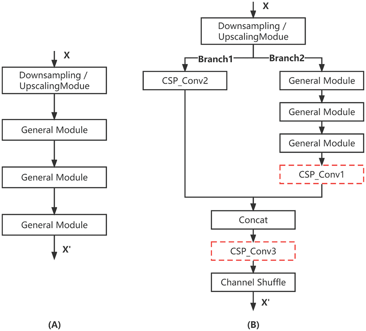
Figure 10: CSP network structure. (A) Original stage; (B) CSP stage

2.3 Model Training

To compare the effect of model improvement before and after, we take the comparison between ShuffleNetV2 (baseline) and ShuffleNet_SE as an example.

2.3.1 Experimental Environment Configuration

The experimental software environment is Windows10 (64-bit) operating system, Python language (Python 3.6), and PyTorch framework. The computer memory is 24 GB, equipped with Intel (R) Core (TM) i7-8550U CPU @ 1.80 GHz 1.99 GHz quad-core processor, and the graphics card is Nvidia MX150 with 4 GB of video memory.

2.3.2 Model Parameter Settings

The ShuffleNet_SE model is used as the standard for model parameter setting. The initial learning rate is 0.01, the learning rate decay mode is exponential decay, and the parameter is set to 0.9; the training period is set to 20, the batch size is set to 16, and the SGD algorithm is used to optimize the training process to avoid overfitting or falling into a local optimum. The image preprocessing method and training details of the experiments in this paper are all adopted in the same way.

Setting of Epoch

Epoch represents the number of times the dataset is trained completely, and the appropriate number of training times is important for the convergence of the model fit, especially when the data is too large, one epoch is not enough to update the weights, and when the parameter values are too large, overfitting will also occur. In this paper, the simulation is carried out for epoch values of 15, 20, and 30, respectively, and the results are shown in Table 2, with batch size set to 16. The corresponding curves are shown in Fig. 11. It can be seen that the model converges faster when the parameter is 20, and the accuracy of the validation set reaches 99.9%, so it is no longer meaningful to increase the parameter value.

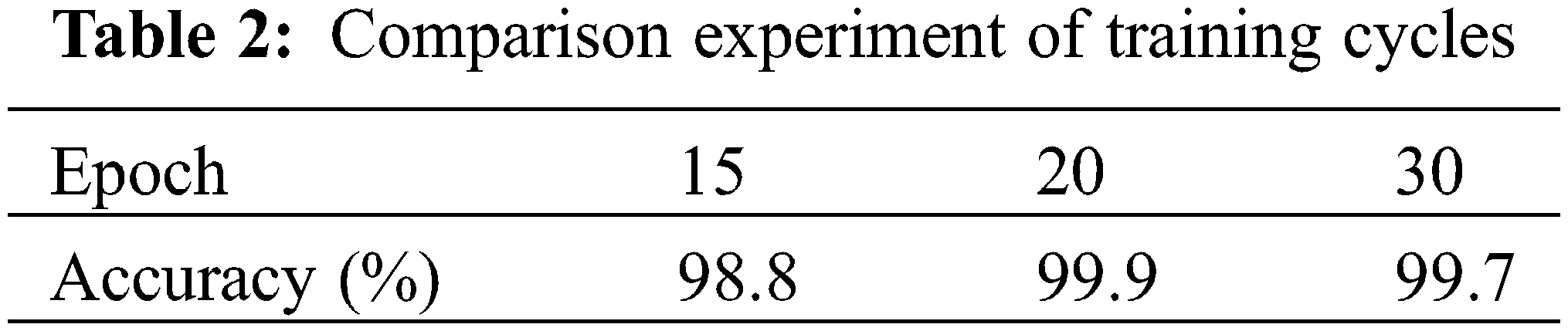
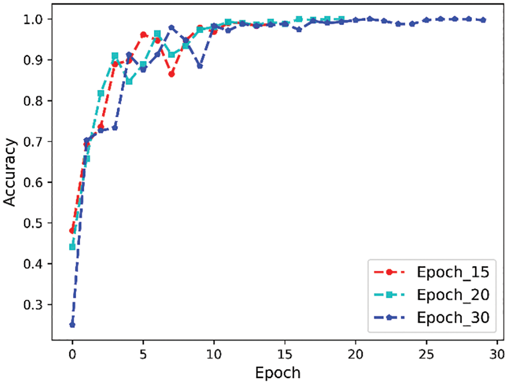
Figure 11: Epoch comparison experiment

3  Theory

3.1 Principle of Attention Mechanism and Derivation of Formula

The specific computation process of the attention mechanism can be summarized into two processes. The first is to calculate the weight coefficients based on the query and key. The second is to weight the summation of value based on the weight coefficients. The first process can be subdivided into two stages. The first stage calculates the similarity or relevance of both based on the query and key. The second stage normalizes the original score of the first stage. In this way, the computational process of attention can be abstracted into three stages as shown in Fig. 12.

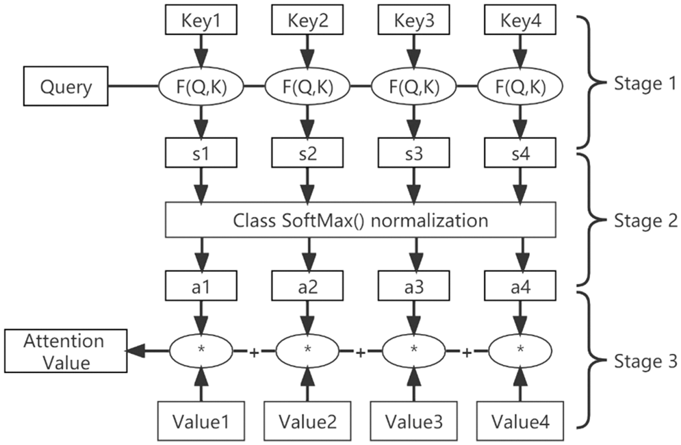
Figure 12: Three-stage calculation of the attention process

In the first stage, different functions and computer mechanisms can be introduced to calculate the similarity or correlation between a query and a certain keyi, based on the most common methods consisting of finding the vector dot product of the two to find the value, as shown in Eq. (1).

Similarity(Query,Keyi)=Query∗Keyi (1)

The scores generated in the first stage have different ranges of values depending on the specific method of generation. In the second stage, a softmax-like calculation is used to numerically transform the scores in the first stage. On the one hand, the scores in the first stage can be normalized to organize the original calculated scores into a probability distribution with the sum of all element weights being 1. On the other hand, it can also highlight more through the inherent mechanism of softmax weights of important elements. It is generally calculated using Eq. (2).

ai=Softmax(Simi)=eSimi∑j=1Lx⁡eSimi (2)

The calculation result ai in the second stage is the weight coefficient corresponding to valuei, and then the weighted summation is performed to obtain the attention value, as shown in Eq. (3).

Attention(Query,Source)=∑i=1Lx⁡ai×Valuei (3)

Through the above three stages of calculation, the attention value for the query can be found, and most of the current specific attention mechanism calculation methods are in line with the above three-stage abstract calculation process.

3.2 Model Evaluation Metrics

Precision-Recall is a metric used to evaluate the quality of the model output. It is a useful indicator of prediction success when the categories are unbalanced. In information retrieval, Precision is a measure of the relevance of results, while Recall is a measure of how many truly relevant results are returned. Accuracy is the difference between the average of each independent prediction and the known true value of the data. These metrics are defined as follows:

(1) If an instance is a positive class, but is predicted to be a positive class, it is a true positive class (True Positive, TP).

(2) If an instance is a negative class but is predicted to be a negative class, it is a true negative class (True Negative, TN).

(3) If an instance is a negative class, but is predicted to be a positive class, it is a false positive class (False Positive, FP).

(4) If an instance is a positive class, but is predicted to be a negative class, it is a false negative class (False Negative, FN).

Precision (P) is defined as the number of true positive classes (TP) over the number of true positive classes (TP) plus the number of false positive classes (FP), as shown in Eq. (4).

P=TPTP+FP (4)

Recall (R) is defined as the number of true positive classes (TP) over the number of true positive classes (TP) plus the number of false negative classes (FN), as shown in Eq. (5).

R=TPTP+FN (5)

Accuracy (A) is defined as the number of correctly classified samples as a percentage of the total number of samples, as shown in Eq. (6).

A=TP+TNTP+TN+FP+FN (6)

3.3 Loss Function

The loss function is used to evaluate the degree of inconsistency between the predicted value of the model Y^=f(x) and the true value Y. It is a non-negative real-valued function. It is usually represented by L(Y,f(x)) , and the smaller the loss function, the better the performance of the model. Let there is always a sample set of N samples as (X,Y)=(xi,yi),yi,i∈[1,N] is the true value of sample i, yi^=f(xi),i∈[1,N] is the predicted value of sample i, and f is the classification function. The total loss function is shown in Eq. (7).

L=∑i=1N⁡l(yi,yi^) (7)

4  Experimental Results and Discussion

4.1 Results

4.1.1 Model Evaluation

Precision Analysis

Precision is a measure of the relevance of the results, and the precision comparison curve is shown in Fig. 13. It can be seen that the final precision before the model improvement is 89% and the final precision after the model improvement is 90%.

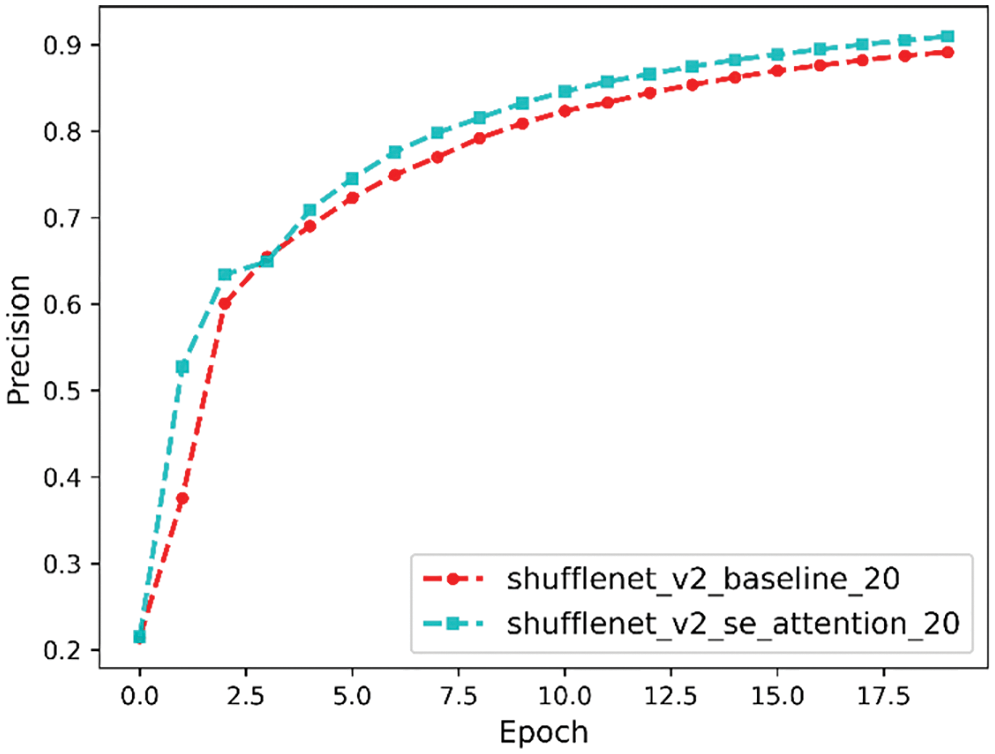
Figure 13: Precision comparison curve

Recall Analysis

Recall is a measure of how many truly relevant results are returned, and the recall comparison curve is shown in Fig. 14. It can be seen that the final recall before the model improvement is 88% and after the model improvement the final recall is 90%.

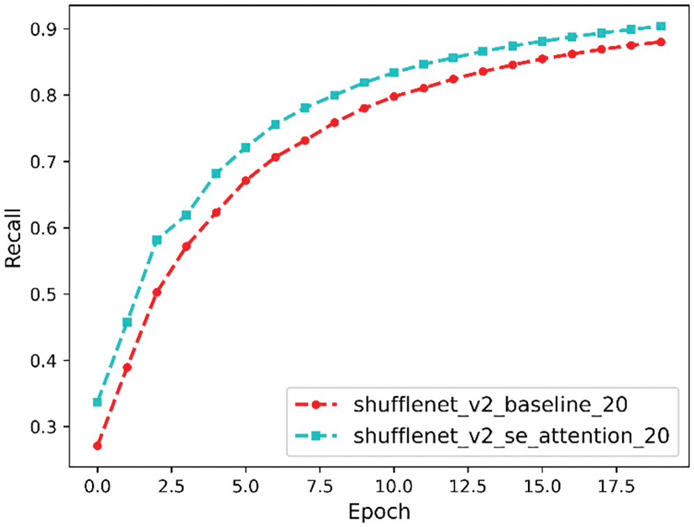
Figure 14: Recall comparison curve

Accuracy Analysis

Accuracy is our most common evaluation metric. Usually, a higher accuracy indicates a better model, and the accuracy comparison curve is shown in Fig. 15. From it, we can see that the final accuracy before model improvement is 97%, and the final accuracy after model improvement is 99%.

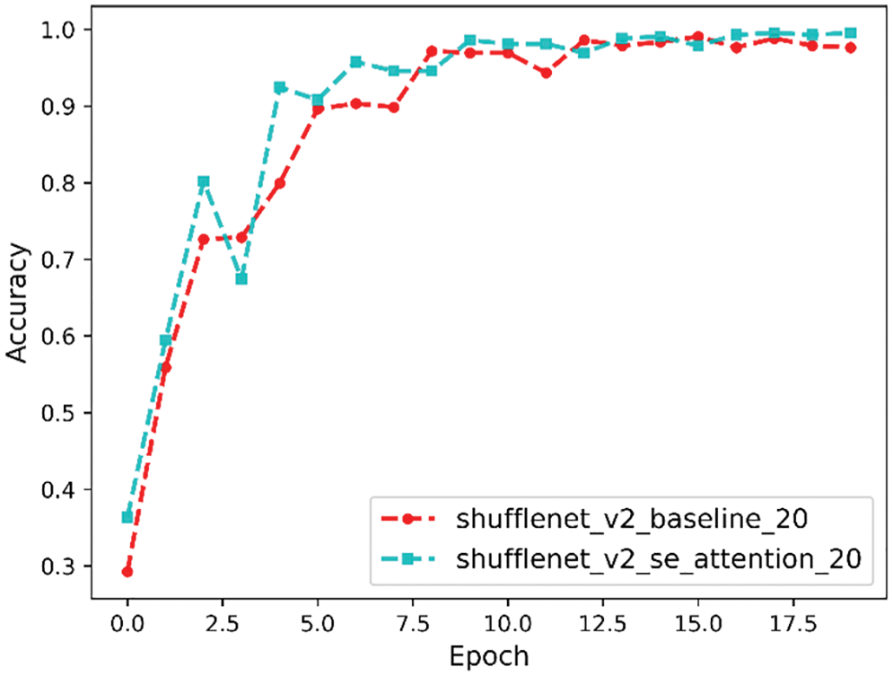
Figure 15: Accuracy comparison curve

Loss Analysis

The loss function is a metric used to evaluate the degree of inconsistency between the predicted value Y^=f(x) of the model and the true value Y. It is a non-negative real-valued function, which is usually denoted by L(Y,f(x)) . The smaller the loss function indicates the better the performance of the model. The loss value comparison curve is shown in Fig. 16. It can be seen that the loss value curve decreases faster after the model improvement than the baseline version, and the final loss value is smaller than that of the baseline version.

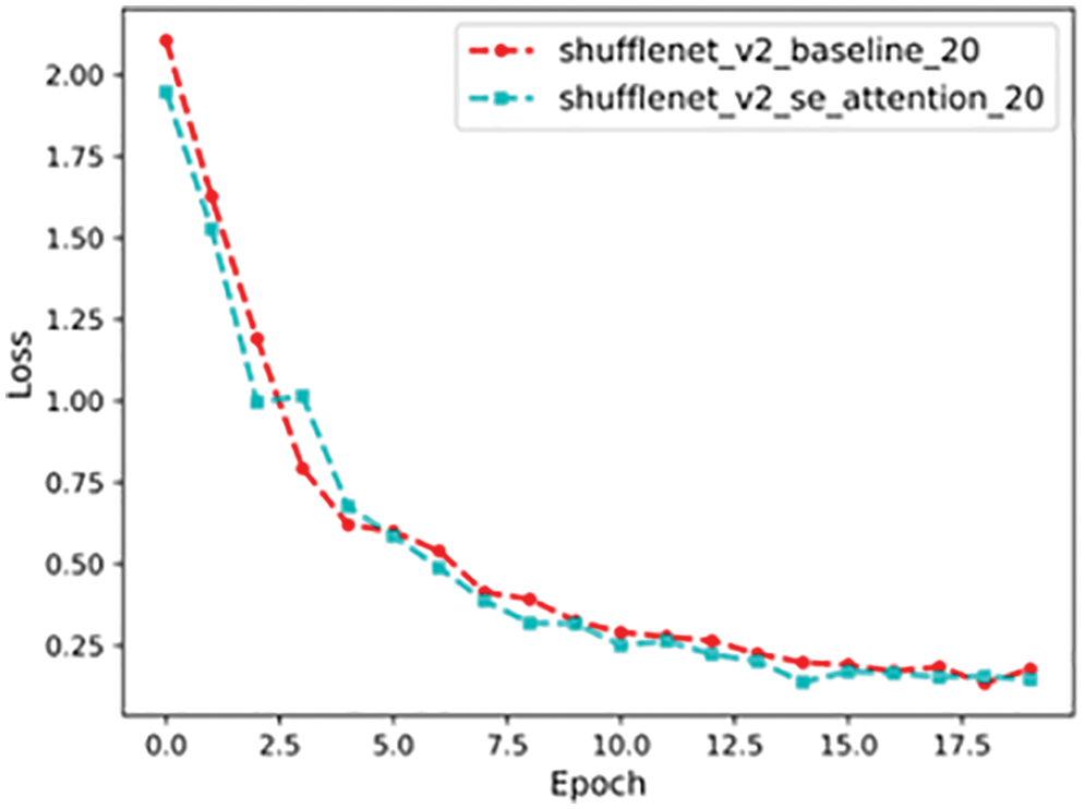
Figure 16: Loss value comparison curve

Confusion Matrix

Confusion matrix is a tool that is used to evaluate the accuracy of the classification results of each stacked generation during the algorithm learning process. As shown in Fig. 17, the confusion matrix of the current classification status of each category is listed after 20 overlapping generations, where the horizontal axis is the experimental predicted classification, and the vertical axis is the real classification, where the sum of the number of each row is the real number of the category. For example, the sum of the first row is 1,100, representing the real existence of 1,100 plant 0 categories, the diagonal line represents the model predicted correctly, while the other positions represent the prediction error. A confusion matrix can quickly help us to analyze the misclassification of each category, thus helping us to analyze the adjustment.

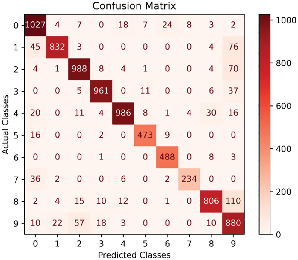
Figure 17: Confusion matrix

10-fold cross-validation

To better evaluate the performance of the models, we mixed the training and test sets and trained the models using the 10-fold cross-validation method, the core idea of which is to divide the dataset several times and average the results of multiple evaluations, thus eliminating the adverse effects caused by the imbalance of data division in a single division, the experimental results are shown in Fig. 18, from which we can see that the average accuracy of the six models has improved relative to the baseline version, among which the average precision of ShuffleNet_LiteConv and ShuffleNet_CSP models has been improved more obviously, and the optimization has been achieved in terms of model performance.

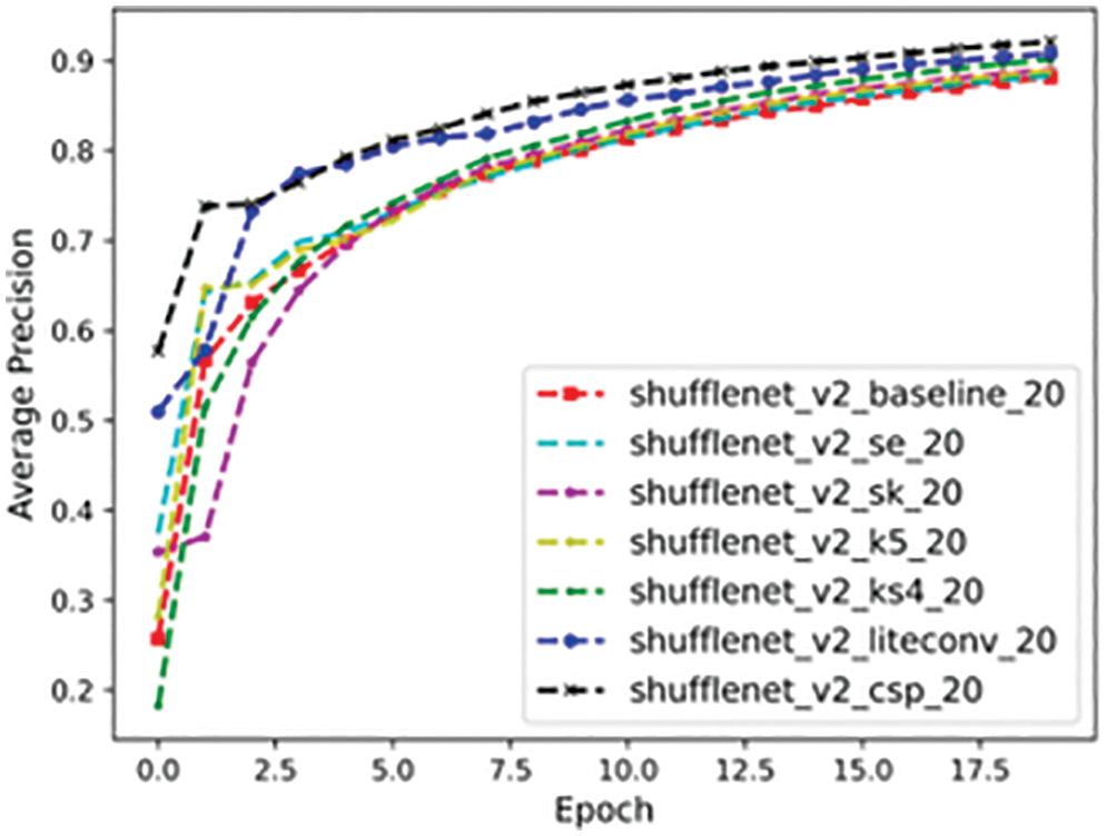
Figure 18: 10-fold cross-validation results of our model

4.1.2 Comparison of Different Models

ShuffleNet_SE, ShuffleNet_SK, ShuffleNet_K5, ShuffleNet_Ks4, ShuffleNet_LiteConv, and ShuffleNet_CSP were trained on the TJAU10 dataset respectively, and their final precision, parameter size, measured FLOPs, and model running time are compared with ShuffleNetV2 of baseline. The results are shown in Table 3.

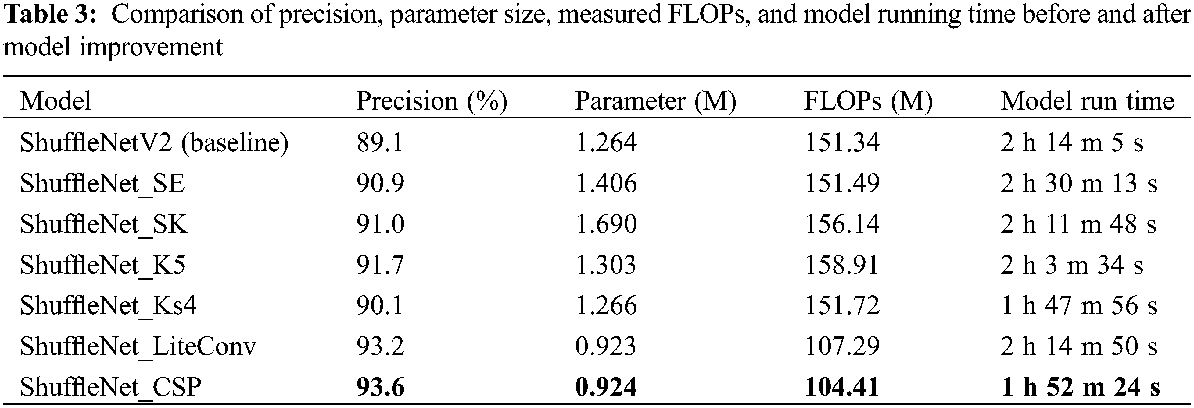
From the perspective of boosting accuracy, ShuffleNet_K5 has the best result, the model running time is shorter than both SE and SK with the addition of the attention mechanism, but the number of parameters and computation are elevated. ShuffleNet_Ks4 improves the precision over ShuffleNetV2 (baseline) with basically the same computation and parameter size of 1.1%, and the model running time is also reduced more significantly. It indicates that the gain of the attention mechanism is not obvious in the lightweight network, and not as high as the gain from directly boosting the convolution kernel of the depthwise convolution. In terms of reducing computation, the ShuffleNet_CSP network is the most effective as can be seen from Table 3, and the streamlined 1 * 1 convolution reduces the computation by about 31% without reducing the precision. The parameter size and model running time are reduced, and the precision improvement is also obvious. The main reason is that ShuffleNetV2 itself already uses the blocking process of splitting and then concatenating in the input channel, which is the same as CSP, except that CSP is based on a stage and ShuffleNetV2 is based on a block. In summary, if we want to improve the accuracy, expanding the convolution kernel is the easiest and most effective, and the computational effort is only increased by 5%. If we want to reduce the computational effort, then the best result is achieved by clipping the 1 * 1 convolution.

To select a more suitable improved model, the six improved network models were tested separately with other CNN models on the TJAU10 dataset under the same experimental conditions. The results of recognition accuracy on the test set are shown in Table 4. It can be seen that all six improved network models are better than the other CNN models. Among them, ShuffleNet_LiteConv recognition accuracy is the highest up to 98.3%, which is higher than the other five improved models, and the improvement is 9.6% higher than ShuffleNetV2 (baseline) model. Therefore, ShuffleNet_LiteConv was selected as the final recognition model in this study. Several plant images were selected for prediction, and Fig. 19 shows the results of ShuffleNet_LiteConv model for plant species recognition.

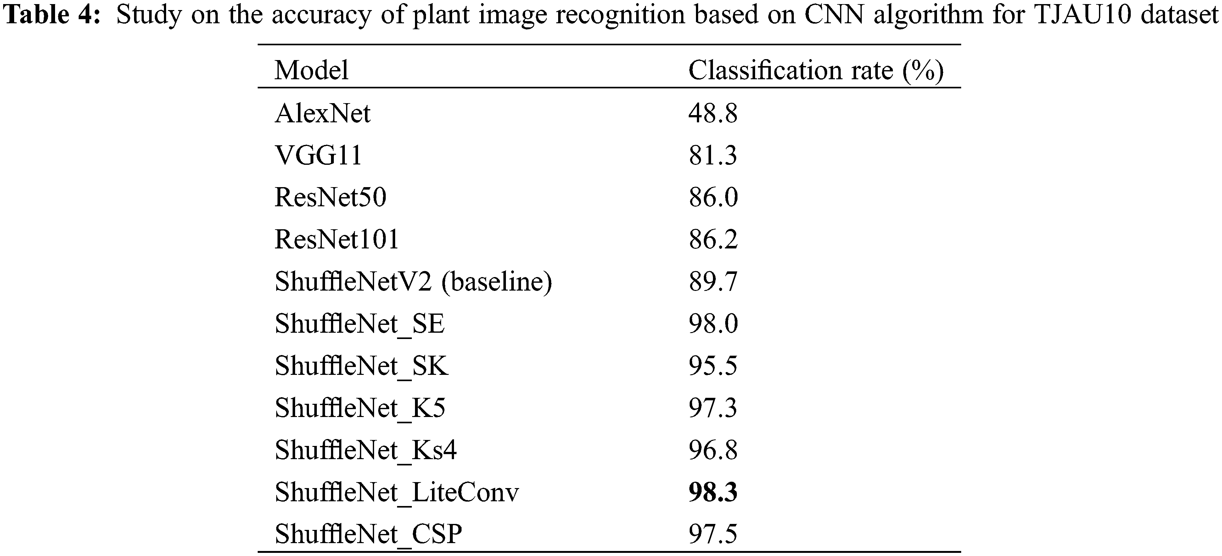
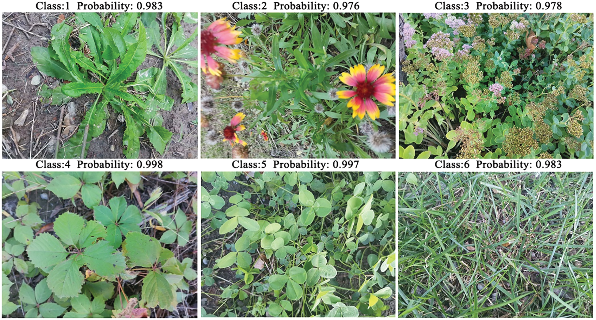
Figure 19: Recognition result

4.2 Discussion

The CNN-based approach for feature extraction and classification under the same architecture achieves good results because it has a convolutional input layer, which acts as a self-learning feature extractor that can learn the optimal features directly from the original pixels of the input image, and the integrated features learned are not limited to shape, texture, or color, but also extend to specific kinds of leaf features, such as structural split, leaf tip, leaf base, leaf margin types, etc. [42–44]. The shortcomings are the lack of actual training samples and the large amount of time required to train the network. Traditional plant species recognition methods are generally not applicable to plant images with a large number of species and complex backgrounds. CNN-based methods have made an important contribution to large-scale plant species recognition in natural environments [45].

This paper introduces a plant species recognition method based on an improved convolutional neural network and its importance. Among the model improvements, the ShuffleNet_K5 model is the best from the perspective of improving precision, with better model runtime than both the model with the attention mechanism SE and SK, but higher parameter size and computation. ShuffleNet_Ks4 improves precision by 1.1% over ShuffleNetV2 (baseline) with essentially the same parameter size and computational effort, and the model running time is the least among the four improved precision models. In terms of reducing computation, the ShuffleNet_CSP model has the most obvious effect, with reduced parameter size and model running time, and more obvious precision improvement, but the precision of plant image recognition on the overall test set is not as good as the ShuffleNet_LiteConv model. In general, each of the six models has its advantages and disadvantages, and all of them achieve the purpose of model optimization to different degrees. The deep learning algorithm based on the convolutional neural network can learn plant image features independently, reduce human intervention, exclude noise interference for natural background plant images, etc., and improve the image recognition rate.

Although the advantages of changing the network structure approach have been seen. However, there are many ways to modify the network structure to improve the generalization ability and reduce computation. For example, we can try to change the number of layers and width of the neural network, etc. They may also obtain better results.

5  Conclusion and Future Directions

Plants have a close relationship with human beings and the environment they live in. How to quickly identify unknown plants without relevant expertise is an important and difficult task because there are a large number of plant species with different leaves that vary greatly between species and are similar within species. With the development of the Internet, computer hardware and software, image processing, and pattern recognition techniques, automatic plant identification based on image processing techniques has become possible. In this paper, we present that CNNs can accurately classify plants in natural environments by improving the network structure for better feature extraction and reducing the complexity of the network with improved accuracy. Experiments show that the improved network can obtain better features, the classification accuracy of the improved model is up to 98.3%, the recognition precision reaches up to 93.6%, the highest increase in recognition precision is 5.1%, and the computational effort is reduced by about 31% compared to the original model. However, our method still has some drawbacks, such as the small variety of plant images for training and the lack of development of a visualization application platform. Therefore, in future work, plant image data of more species can be collected and an attempt can be made to deploy this lightweight model on mobile, embedded, and PC devices, respectively, to test the recognition of plant species in large-scale natural environments to improve the usage.

Authorship: The authors confirm contribution to the paper as follows: study conception and design: C.Y., T.L.; data collection: C.Y., S.S., F.G., R.Z.; analysis and interpretation of results: C.Y.; draft manuscript preparation: C.Y. All authors reviewed the results and approved the final version of the manuscript.

Funding Statement: This study was supported by the Key Project Supported by Science and Technology of Tianjin Key Research and Development Plan [Grant No. 20YFZCSN00220], Tianjin Science and Technology Plan Project [Grant No. 21YFSNSN00040], Central Government Guides Local Science and Technology Development Project [Grant No. 21ZYCGSN00590], and Inner Mongolia Autonomous Region Department of Science and Technology Project [Grant No. 2020GG0068].

Conflicts of Interest: The authors declare that they have no conflicts of interest to report regarding the present study.

References

 1.  Zhang, S., Huang, W., Huang, Y. (2020). Plant species recognition methods using leaf image: Overview. Neurocomputing, 408(12), 246–272. DOI 10.1016/j.neucom.2019.09.113. [Google Scholar] [CrossRef]

 2.  Pimm, S. L., Joppa, L. N. (2015). How many plant species are there, where are they, and at what rate are they going extinct? Annals of the Missouri Botanical Garden, 100(3), 170–176. DOI 10.3417/2012018. [Google Scholar] [CrossRef]

 3.  Zhao, Z. Q., Ma, L. H., Cheung, Y. (2015). ApLeaf: An efficient android-based plant leaf identification system. Neurocomputing, 151(1), 1112–1119. DOI 10.1016/j.neucom.2014.02.077. [Google Scholar] [CrossRef]

 4.  Yang, C. (2021). Plant leaf recognition by integrating shape and texture features. Pattern Recognition, 112(1), 107809. DOI 10.1016/j.patcog.2020.107809. [Google Scholar] [CrossRef]

 5.  Messaoud, S., Bouaafia, S., Maraoui, A. (2022). Deep convolutional neural networks-based hardware-software on-chip system for computer vision application. Computers & Electrical Engineering, 98(1), 107671. DOI 10.1016/j.compeleceng.2021.107671. [Google Scholar] [CrossRef]

 6.  Jang, G., Lee, J., Lee, J. G. (2020). Distributed fine-tuning of CNNs for image retrieval on multiple mobile devices. Pervasive and Mobile Computing, 64(7), 101134. DOI 10.1016/j.pmcj.2020.101134. [Google Scholar] [CrossRef]

 7.  Torres, H. R., Morais, P., Oliveira, B. (2022). A review of image processing methods for fetal head and brain analysis in ultrasound images. Computer Methods and Programs in Biomedicine, 215(3), 106629. DOI 10.1016/j.cmpb.2022.106629. [Google Scholar] [CrossRef]

 8.  Abumalloh, R. A., Nilashi, M., Ismail, M. Y. (2022). Medical image processing and COVID-19: A literature review and bibliometric analysis. Journal of Infection and Public Health, 15(1), 75–93. DOI 10.1016/j.jiph.2021.11.013. [Google Scholar] [CrossRef]

 9.  Alanne, K., Sierla, S. (2022). An overview of machine learning applications for smart buildings. Sustainable Cities and Society, 76(1), 103445. DOI 10.1016/j.scs.2021.103445. [Google Scholar] [CrossRef]

10. Zhang, S., Zhang, C., Huang, W. (2018). Integrating leaf and flower by local discriminant CCA for plant species recognition. Computers and Electronics in Agriculture, 155(12), 150–156. DOI 10.1016/j.compag.2018.10.018. [Google Scholar] [CrossRef]

11. Toğaçar, M., Ergen, B., Cömert, Z. (2020). Classification of flower species by using features extracted from the intersection of feature selection methods in convolutional neural network models. Measurement, 158, 107703. DOI 10.1016/j.measurement.2020.107703. [Google Scholar] [CrossRef]

12. Loddo, A., Loddo, M., di Ruberto, C. (2021). A novel deep learning based approach for seed image classification and retrieval. Computers and Electronics in Agriculture, 187(1), 106269. DOI 10.1016/j.compag.2021.106269. [Google Scholar] [CrossRef]

13. Tiwari, V., Joshi, R. C., Dutta, M. K. (2021). Dense convolutional neural networks based multiclass plant disease detection and classification using leaf images. Ecological Informatics, 63, 101289. DOI 10.1016/j.ecoinf.2021.101289. [Google Scholar] [CrossRef]

14. Lukic, M., Tuba, E., Tuba, M. (2017). Leaf recognition algorithm using support vector machine with Hu moments and local binary patterns. 2017 IEEE 15th International Symposium on Applied Machine Intelligence and Informatics (SAMI), pp. 000485–000490. Herl'any, Slovakia. DOI 10.1109/SAMI.2017.7880358. [Google Scholar] [CrossRef]

15. Wang, B., Gao, Y., Sun, C. (2017). Can walking and measuring along chord bunches better describe leaf shapes? 2017 IEEE Conference on Computer Vision and Pattern Recognition (CVPR), pp. 2047–2056. Honolulu, HI. DOI 10.1109/CVPR.2017.221. [Google Scholar] [CrossRef]

16. Alamoudi, S., Hong, X., Wei, H. (2020). Plant leaf recognition using texture features and semi-supervised spherical K-means clustering. 2020 International Joint Conference on Neural Networks (IJCNN), pp. 1–8. Glasgow, UK. DOI 10.1109/IJCNN48605.2020.9207386. [Google Scholar] [CrossRef]

17. Zhao, C., Chan, S. S. F., Cham, W. K. (2015). Plant identification using leaf shapes—A pattern counting approach. Pattern Recognition, 48(10), 3203–3215. DOI 10.1016/j.patcog.2015.04.004. [Google Scholar] [CrossRef]

18. Metre, V., Ghorpade, J. (2013). An overview of the research on texture based plant leaf classification. International Journal of Computer Science and Network, 2(3). DOI 10.48550/arXiv.1306.4345. [Google Scholar] [CrossRef]

19. Yuan, P., Qian, S., Zhai, Z. (2022). Study of chrysanthemum image phenotype on-line classification based on transfer learning and bilinear convolutional neural network. Computers and Electronics in Agriculture, 194(12), 106679. DOI 10.1016/j.compag.2021.106679. [Google Scholar] [CrossRef]

20. Guru, D. S., Sharath Kumar, Y. H., Manjunath, S. (2011). Textural features in flower classification. Mathematical and Computer Modelling, 54(3–4), 1030–1036. DOI 10.1016/j.mcm.2010.11.032. [Google Scholar] [CrossRef]

21. Lee, H. H., Hong, K. S. (2017). Automatic recognition of flower species in the natural environment. Image and Vision Computing, 61, 98–114. DOI 10.1016/j.imavis.2017.01.013. [Google Scholar] [CrossRef]

22. Yang, C., Yu, Q. (2019). Multiscale fourier descriptor based on triangular features for shape retrieval. Signal Processing: Image Communication, 71(4), 110–119. DOI 10.1016/j.image.2018.11.004. [Google Scholar] [CrossRef]

23. Salve, P., Yannawar, P., Sardesai, M. (2022). Multimodal plant recognition through hybrid feature fusion technique using imaging and non-imaging hyper-spectral data. Journal of King Saud University-Computer and Information Sciences, 34(1), 1361–1369. DOI 10.1016/j.jksuci.2018.09.018. [Google Scholar] [CrossRef]

24. Schmidhuber, J. (2015). Deep learning in neural networks: An overview. Neural Networks, 61(3), 85–117. DOI 10.1016/j.neunet.2014.09.003. [Google Scholar] [CrossRef]

25. Chang, H., Yang, M., Yang, J. (2016). Learning a structure adaptive dictionary for sparse representation based classification. Neurocomputing, 190(1), 124–131. DOI 10.1016/j.neucom.2016.01.026. [Google Scholar] [CrossRef]

26. Prieto, A., Prieto, B., Ortigosa, E. M. (2016). Neural networks: An overview of early research, current frameworks and new challenges. Neurocomputing, 214(12), 242–268. DOI 10.1016/j.neucom.2016.06.014. [Google Scholar] [CrossRef]

27. Kaviani, S., Sohn, I. (2021). Application of complex systems topologies in artificial neural networks optimization: An overview. Expert Systems with Applications, 180(5439), 115073. DOI 10.1016/j.eswa.2021.115073. [Google Scholar] [CrossRef]

28. Patil, S., Patra, B., Goyal, N. (2021). Recognizing plant species using digitized leaves-a comparative study. 2021 5th International Conference on Trends in Electronics and Informatics (ICOEI), pp. 1138–1143. Tirunelveli, India. DOI 10.1109/ICOEI51242.2021.9453003. [Google Scholar]

29. Wäldchen, J., Mäder, P. (2018). Plant species identification using computer vision techniques: A systematic literature review. Archives of Computational Methods in Engineering, 25(2), 507–543. DOI 10.1007/s11831-016-9206-z. [Google Scholar] [CrossRef]

30. Li, Q., Xiong, D., Shang, M. (2022). Adjusted stochastic gradient descent for latent factor analysis. Information Sciences, 588(1), 196–213. DOI 10.1016/j.ins.2021.12.065. [Google Scholar] [CrossRef]

31. Fjellström, C., Nyström, K. (2022). Deep learning, stochastic gradient descent and diffusion maps. Journal of Computational Mathematics and Data Science, 4(1), 100054. DOI 10.1016/j.jcmds.2022.100054. [Google Scholar] [CrossRef]

32. Mutlu, G., Acı, Ç. İ. (2022). SVM-SMO-SGD: A hybrid-parallel support vector machine algorithm using sequential minimal optimization with stochastic gradient descent. Parallel Computing, 113(4), 102955. DOI 10.1016/j.parco.2022.102955. [Google Scholar] [CrossRef]

33. Ren, L. H., Ye, Z. F., Zhao, Y. P. (2020). A modeling method for aero-engine by combining stochastic gradient descent with support vector regression. Aerospace Science and Technology, 99, 105775. DOI 10.1016/j.ast.2020.105775. [Google Scholar] [CrossRef]

34. Tian, C., Fei, L., Zheng, W. (2020). Deep learning on image denoising: An overview. Neural Networks, 131(11), 251–275. DOI 10.1016/j.neunet.2020.07.025. [Google Scholar] [CrossRef]

35. Li, G., Yang, Y., Qu, X. (2021). A deep learning based image enhancement approach for autonomous driving at night. Knowledge-Based Systems, 213(1), 106617. DOI 10.1016/j.knosys.2020.106617. [Google Scholar] [CrossRef]

36. Veerendra, G., Swaroop, R., Dattu, D. S. (2022). Detecting plant Diseases, quantifying and classifying digital image processing techniques. Materials Today: Proceedings, 51(4), 837–841. DOI 10.1016/j.matpr.2021.06.271. [Google Scholar] [CrossRef]

37. Zhang, X., Zhou, X., Lin, M. (2018). ShuffleNet: An extremely efficient convolutional neural network for mobile devices. 2018 IEEE/CVF Conference on Computer Vision and Pattern Recognition (CVPR), pp. 6848–6856. Salt Lake City, UT, USA. DOI 10.1109/CVPR.2018.00716. [Google Scholar] [CrossRef]

38. Hu, J., Shen, L., Albanie, S. (2019). Squeeze-and-excitation networks. IEEE Transactions on Pattern Analysis and Machine Intelligence, 42(8), 2011–2023. DOI 10.1109/TPAMI.2019.2913372. [Google Scholar] [CrossRef]

39. Li, X., Wang, W., Hu, X. (2019). Selective kernel networks. 2019 IEEE/CVF Conference on Computer Vision and Pattern Recognition (CVPR), pp. 510–519. Long Beach, CA, USA. DOI 10.1109/CVPR.2019.00060. [Google Scholar] [CrossRef]

40. Sandler, M., Howard, A., Zhu, M., Zhmoginov, A., Chen, L. C. (2018). MobileNetV2: Inverted residuals and linear bottlenecks. 2018 IEEE/CVF Conference on Computer Vision and Pattern Recognition (CVPR), pp. 4510–4520. Salt Lake City, UT, USA. DOI 10.1109/CVPR.2018.00474. [Google Scholar] [CrossRef]

41. Wang, C. Y., Liao, H., Wu, Y. H. (2020). CSPNet: A new backbone that can enhance learning capability of CNN. 2020 IEEE/CVF Conference on Computer Vision and Pattern Recognition Workshops (CVPRW), pp. 1571–1580. Seattle, WA, USA. DOI 10.1109/CVPRW50498.2020.00203. [Google Scholar] [CrossRef]

42. Tavakoli, H., Alirezazadeh, P., Hedayatipour, A. (2021). Leaf image-based classification of some common bean cultivars using discriminative convolutional neural networks. Computers and Electronics in Agriculture, 181, 105935. DOI 10.1016/j.compag.2020.105935. [Google Scholar] [CrossRef]

43. Subeesh, A., Bhole, S., Singh, K. (2022). Deep convolutional neural network models for weed detection in polyhouse grown bell peppers. Artificial Intelligence in Agriculture, 6, 47–54. DOI 10.1016/j.aiia.2022.01.002 S2589721722000034. [Google Scholar] [CrossRef]

44. Xu, W., Zhao, L., Li, J. (2022). Detection and classification of tea buds based on deep learning. Computers and Electronics in Agriculture, 192(33), 106547. DOI 10.1016/j.compag.2021.106547. [Google Scholar] [CrossRef]

45. Sachar, S., Kumar, A. (2021). Survey of feature extraction and classification techniques to identify plant through leaves. Expert Systems with Applications, 167(4), 114181. DOI 10.1016/j.eswa.2020.114181. [Google Scholar] [CrossRef]