Improving the Accuracy of Vegetation Index Retrieval for Biomass by Combining Ground-UAV Hyperspectral Data–A New Method for Inner Mongolia Typical Grasslands

1  Introduction

The aboveground biomass (AGB) of grasslands is an important indicator for the sustainable use of grassland resources and assessment of the livestock carrying capacity [1,2]. As an important predictor, AGB can reflect vegetation growth status and gross primary product and is one of the important manifestations of constant grassland quality and grassland carbon sequestration capacity [3,4]. Rapid and accurate estimation of grassland AGB is crucial for regional grassland management and sustainable development [5,6], making it a research hotspot in the field of the grassland ecosystem. The traditional field survey methods can achieve high-precision results in estimating grassland biomass. However, this process is highly destructive, with a small range of applications and high labor, material, and time costs [7–9].

Remote sensing technology allows rapid, efficient, and dynamic observation of grassland vegetation at a macroscopic scale. By establishing regression models between field measurement values and vegetation indices, the estimates of regional grassland AGB can be quickly obtained [10–12]. Vegetation index (VI) is a linear or nonlinear combination of two or more spectral bands. It can reduce or eliminate the influence of background noise on the spectral information of grassland vegetation canopy, thus enhancing the estimation of vegetation structure [13]. Therefore, it has been widely used in the field of remote sensing inversion of grassland biomass. Zhao et al. [14] calculated vegetation indices such as the Normalized Difference Vegetation Index (NDVI) and Enhanced Vegetation Index (EVI) using Moderate-resolution Imaging Spectroradiometer (MODIS) data and A regression model was established with aboveground biomass to invert the aboveground biomass and changes of Xilingol Grassland in Northern China. Liang et al. [15] calculated 12 vegetation indices such as NDVI, EVI and Ratio Vegetation Index (RVI) to establish a regression model of alpine grassland biomass in the Three-River Headwaters Region. The results showed that NDVI had the best correlation with AGB of alpine grassland, and the model accuracy was the best. John et al. [16] established a rule-based regression tree model based on the vegetation index obtained from MODIS-adjusted reflectance data to invert the spatial and temporal distribution of AGB in Mongolia and Inner Mongolia grasslands in China. Although these studies have obtained accurate AGB estimates using statistical models based on vegetation indices, there are still some shortcomings. When the original spectral information of canopy vegetation is directly used to calculate the vegetation index to invert AGB, the model is easily saturated. Therefore, it is necessary to deeply mine the original spectral information and analyze the characteristic parameters to improve the accuracy of AGB inversion.

The traditional multispectral vegetation indices are limited to the characteristic bands of red, near-red, and mid-infrared. These vegetation indices have the disadvantages of small band numbers, large bandwidths, and restricted wavelength positions, which cannot accurately reflect biomass characteristics [17,18]. Hyperspectral remote sensing, on the other hand, has a high spectral resolution and spectral information in hundreds of bands. It provides detailed and continuous spectral profiles and solves problems that cannot be addressed in multispectral broadband studies [19–21]. In the study of non-imaging spectroscopy, Zhang et al. [22] measured the spectra of four types of grass (including Leymus chinensis, Stipa capillata, Carex pediformis, and Cleistogenes) based on a ground ASD spectrometer in Xilingol, Inner Mongolia. Four hyperspectral feature parameters were selected through correlation analysis and principal component analysis. In addition, a neural network model was used to identify grass species, with an accuracy of up to 80%. Through correlation analysis and regression analysis, Kong et al. [9] developed a multi-scale remote sensing inversion model of alpine grassland biomass based on ground-measured spectral data and dry biomass. The results showed that the original bands at 550, 680, 860, and 900 nm and their combined forms were significantly correlated with biomass. The remote sensing biomass estimation model based on the normalized values of green peak reflectance and red valley reflectance and two spectral features of NDVI exhibited a high inversion accuracy, with R2 of 0.869. Ulan-Tuya et al. [23] used ASD spectral data to extract 13 hyperspectral feature variables with ground sample data to construct a model. The results showed that the correlation coefficient of the ratio between reflectance, blue-edge area, and red-edge area of the red valley reached 0.86. Moreover, the correlation coefficient between the Atmospherically Resistant Vegetation Index (ARVI) and grassland biomass reached 0.85, which was the highest among the eight vegetation indices. The development of UAV imaging technology offers new possibilities for hyperspectral remote sensing. Its hyperspectral camera has low cost and excellent efficiency, allowing rapid and efficient acquisition of hyperspectral imaging data with high resolution through sub-cloud image acquisition [24–27]. On this basis, relevant studies have been conducted by scholars. Yang et al. [28] used UAV hyperspectral data to estimate maize biomass. The Kappa coefficient was 0.69 after fitting with the Convolutional Neural Networks (CNN) model, with higher prediction accuracy by combining spectral and image information. Li et al. [29] used UAV to acquire hyperspectral imaging data of the potato canopy at two growth stages to establish AGB and crop yield prediction models. The R2 of the fitted model for the four narrow-band vegetation indices was 0.9. In order to develop models for estimating fresh and dry biomass, Wengert et al. [30] collected UAV hyperspectral data in eight grassland sites in North Hesse, Germany. The yield distribution map was developed with the best model, providing new technical support for AGB monitoring with high prediction accuracy. There have been many studies on the estimation of grassland AGB based on ground remote sensing and low-altitude UAV remote sensing, but few studies have combined the two. The single remote sensing data source inversion of grassland biomass has deficiencies in accuracy and plant information extraction richness, which will affect the accuracy of the inversion results. Therefore, it is necessary to combine multi-source data to monitor grassland growth.

In addition to high spectral resolution and rich information, hyperspectral remote sensing data is also an important means to monitor grassland conditions. However, the hyperspectral data has many bands, and the spectral information may have disadvantages such as invalidity, redundancy, and overlap, resulting in unstable full-band inversion models and difficulties in improving model accuracy [31]. Therefore, the selection of key wavelength variables is essential. In the above studies, several scholars used vegetation indices or a combination of vegetation indices and analysis methods to estimate AGB production [32,33]. Although good inversion accuracy was achieved, the original spectral information was not deeply mined, making it difficult to further improve the prediction performance of the model by filtering, redundancy, and collinearity information. Furthermore, inner Mongolia grassland is characterized by wide area and spatial heterogeneity. In order to quickly understand the grassland conditions across regions, it is necessary to construct the model in different regions.

Therefore, establishing an AGB estimation model based on hyperspectral data at the regional scale is important for the deep mining of spectral information [34].

Currently, there are two main types of modeling inversion methods for biomass. One is the statistical modeling method, which uses spectral reflectance or some transformation of reflectance (e.g., vegetation index) as the independent variable, biomass obtained from field trials as the dependent variable, and establishes an inversion model based on the correlation between the two, and is widely used in studies of inverted biomass with the advantages of being easy to implement and simple and straightforward [35]. Although the statistical method is simple in structure and easy to compute, the difference in sensitivity of the method to vegetation type, soil background, and climatic influences, as well as a certain degree of saturation of vegetation indices in the inversion process, results in a relatively poor generalisability of the model; The second is the physical modeling method, which is based on the non-Lambertian characteristics of the vegetation canopy, and simulates the radiative transfer process within the canopy to achieve the inversion of biomass based on the consideration of the mechanism of light and foliage action, so the model does not change according to the different vegetation types, and the applicability is relatively good. However, the physical modeling method is relatively complex, the model requires many input parameters and some of them are not easy to obtain, and the inversion process is relatively difficult [36,37].

The saturation phenomenon of vegetation indices results from a significant decrease in the sensitivity of vegetation indices to changes in biomass under conditions of high vegetation cover, most typically in the case of NDVI, which usually constrains the accuracy of models [38]. In order to solve this problem, some scholars have studied the improvement of the vegetation index. Huete et al. [39] proposed SAVI, which reduces the disturbance of soil and vegetation canopy background. Liu et al. [40] introduced blue and green light bands to construct a moderated normalized vegetation index (ANDVI) containing four spectral bands, blue, green, red and near-infrared, which increased the universality and robustness compared to NDVI. Some scholars constructed biomass estimation models with multiple vegetation index characteristics, Gao et al. [41] compared the potential of the multivariate linear regression model and univariate nonlinear model in AGB estimation, and the results showed that the multivariate model has a better accuracy, but due to the multivariate covariate problem, the multivariate model is prone to overfitting phenomenon, and there are some deficiencies in the stability of the model. This study aimed to analyze the hyperspectral curve of grassland canopy in typical grassland of Inner Mongolia by ground remote sensing data, screen out sensitive bands, and calculate vegetation index, so as to establish an AGB inversion model combining ground non-imaging and UAV imaging. This would allow to improve the inversion accuracy of biomass vegetation index and achieve accurate and rapid estimation of grassland AGB in the region. The results can provide a theoretical basis for the strategic adjustment and management optimization of grassland ecosystems in Inner Mongolia. The specific objectives were as follows:

1.   Grassland canopy spectral characterization was conducted. It involves the first- and second-order derivative changes of the raw spectra, logarithmic changes, trilateral characterization, and correlation analysis with dry and fresh weights of AGB to screen out sensitive bands.

2.   Based on the above sensitive bands, four narrow-band vegetation indices were established. In addition, the remote sensing estimation models of ground hyperspectral and UAV imaging hyperspectral were developed for the air-ground experiment of AGB in typical grasslands of Inner Mongolia.

3.   The determination coefficient (R2), root mean square error (RMSE), and estimated relative error (REE) were used to verify the accuracy of the inversion model. Finally, the AGB monitoring method suitable for typical grassland in Inner Mongolia was obtained.

2  Materials and Methods

2.1 Research Area

The research area is in a typical grassland in Xilingol League, Inner Mongolia Autonomous Region, China. The research site is the Grassland Ecology Research Base of Inner Mongolia University (N44°12.621′, E116°15.446′), Elevation is about 900 m.a.s.l. which has a temperate semi-arid climate with an average annual temperature of 3.5°C, an average annual precipitation of 270 mm, and an average precipitation of 229 mm from May to September. The research area has abundant grassland resources, favorable livestock conditions, and typical grassland vegetation, with the soil type of chestnut-calcium soil. The most common plants include Leymus chinensis, Stipa spartea, and Cleistogenes squarrosa [42,43].

2.2 Data Source

Field quadrat data were collected in the study area in July and August 2021. First, a 1 m × 1 m sample plot was established for each treatment plot, followed by random sampling with three replicates in each sample plot. The plant species, total AGB, and the total height of each species in the community were recorded, with 66 sample squares investigated. Finally, the plants of each quadrat were cut off and brought back to the laboratory to weigh the fresh weight. To take the dry weight, samples were put in an oven to 65°C until constant weight was reached. The dried samples were then weighted.

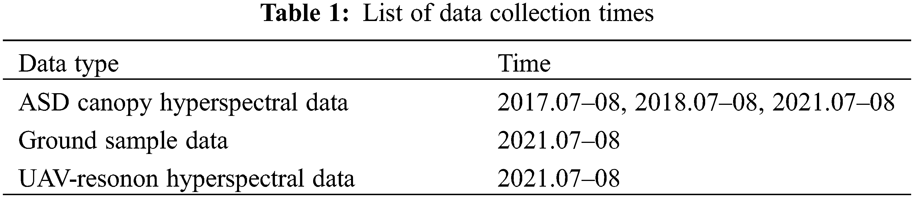
The ASD canopy spectra were divided into two time periods for data collection, which are referenced in Table 1. To obtain canopy reflectance of grassland communities, spectral data were collected from each quadrat using an ASD FieldSpec4 spectrometer. The data was collected between 10 a.m. and 2 p.m. in cloudless, breezy weather. During the measurement, the view angle of the spectrometer was 25°, and the sensor probe was placed vertically downward. To ensure the validity of the spectral data, 10 spectral data were set as one unit before data collection. For each spectral data collected, 10 canopy reflectance spectral curves were automatically recorded in the instrument, and the average value was automatically calculated as the final reflectance data. Three measurements were performed directly above each sample target to exclude abnormal spectral data [44].

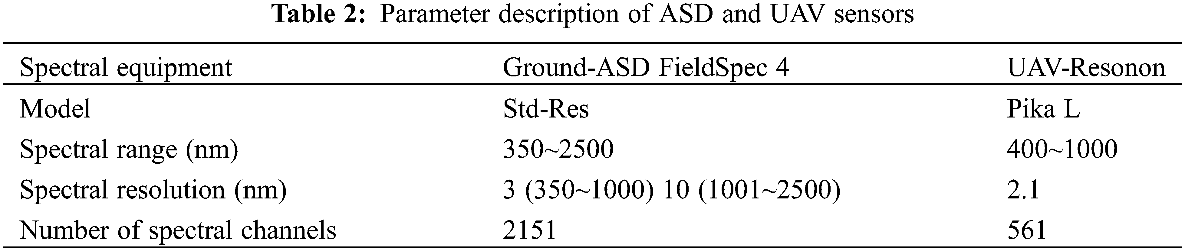
UAV remote sensing data and ground-based ASD spectral data were simultaneously collected in July and August 2021; the parameters of the two different spectroscopic devices were described in Table 2. Hyperspectral remote sensing data of grassland in the research area were obtained by UAV, along with the data of 107 ASD grassland canopy reflectance sample points and the AGB data of 54 sample squares corresponding to the field test as ground verification data.

The UAV used in this study was a DaJiang Innovations (DJI, Uav manufacturer) Matrice 600 Pro with an A3 professional flight controller (Fig. 1a). Flight tasks were created and executed in grid mode in DJI Ground Station Pro, and image acquisition tasks were performed in autonomous mode. The DJI Ronin MX was used to carry an airborne hyperspectral imaging component that keeps the camera at the lowest point during UAV flight. The weight of the platform was 10 kg, the maximum load was 5 kg, and the flight time was 20 min. The flight height was set to 120 m, speed 4 m/s, overlap rate 30%, and spatial resolution 4.5 cm. Then, the UAV was taken off to an open test environment, and the flight was controlled automatically and manually. During the initial and final alignment phases, the test environment was kept open, and the roll and pitch angles of the UAV were kept at 0° to ensure a good alignment.

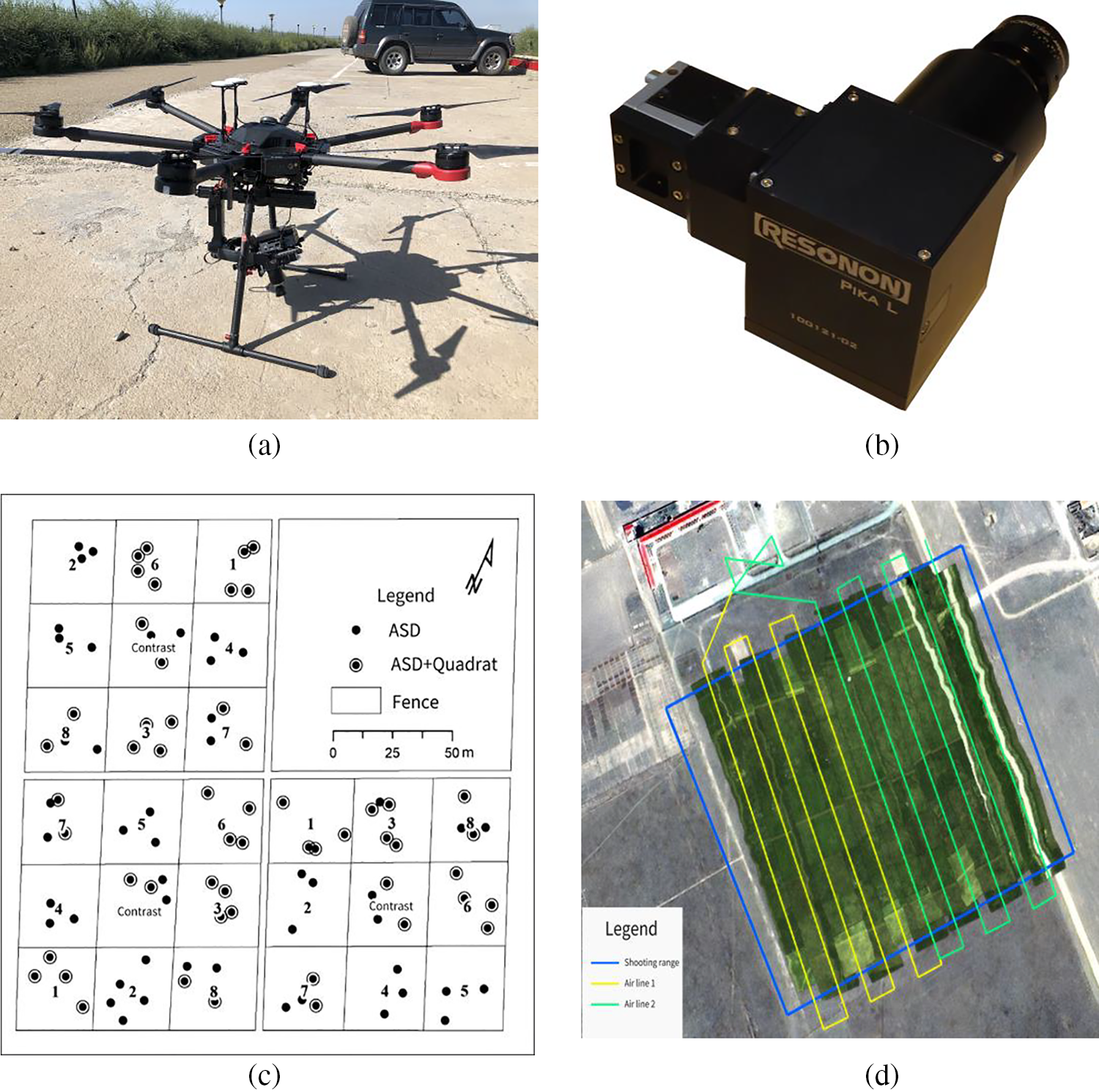
Figure 1: Hyperspectral platform based on UAV. (a) UAV used in the research. (b) Hyperspectral camera; (c) Distribution of field monitoring sample points (The study area was divided into 3 blocks with 9 plots in each block. The ‘1–7’ plot represented different grazing gradients, the ‘8’ plot was mowing, and the ‘contrast’ was blank control.); (d) UAV flight route

Due to the small sample area, the Real-time kinematic (RTK, coordinate setting) measurement system was used for sample point positioning, and the distribution of field measurement points was shown in Fig. 1c. Two flight routes were preset for data collection (Fig. 1d). The flight was automatically controlled using the GS PRO software of DJI UAV. Through the Resonon Ground Station software of the hyperspectral camera (Fig. 1b), relevant flight parameters and sample range data were imported and uploaded to the camera computer, enabling the collaboration of the UAV and camera.

The geometric correction and orthorectification of Resonon data require high-resolution images as reference data, and the DJI Genie 4 image data were collected simultaneously. According to the sample area, the DJI GO 4 software was used to set the route height to 80 m. The route was generated automatically, and the image overlap rate was set to 50% to obtain true color images with a spatial resolution of 2 cm.

2.3 Data Pre-Processing

Highly accurate control points were obtained by collecting sample coordinates and sample plot fence inflection coordinates to fine-tune DJI Genie 4 and Resonon hyperspectral images. The coordinates were imported into the computer through the electronic handbook of RTK. Then, the sample point location map and the boundary map of the fence were generated in ArcMap software, as shown in Fig. 1c.

The camera on the DJI Genie 4 Pro UAV features a 1-inch 20-megapixel image sensor, allowing it to capture 4K/60 fps video and still photos at 14 fps. The DJI GO 4 software controlled the automatic flight to obtain true color images of the sample area. Afterward, the images were processed in PhotoScan software to export orthophoto and Digital Elevation Model (DEM) stitching results (Fig. 2a).

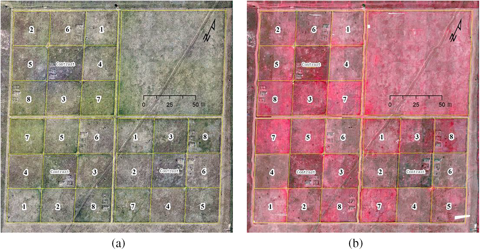
Figure 2: Hyperspectral image data. (a) Mosaic correction image of DJI Genie 4 Pro; (b) Hyperspectral image data of sample plot

Resonon hyperspectral raw data requires pre-processing, such as radiance conversion geometric correction, which can be completed in Spectronon Pro software. When performing the radiance conversion, the raw data were first subjected to dark current correction to convert the K-Type hyperspectral data to radiance brightness values that can be recognized by ENVI image processing software. Next, the average reflectance value was calculated by bringing the data of dark current correction and standard whiteboard reflectance into the equation to obtain the data for each image element. The reflectance data of each cell were averaged as the final reflectance value:

Reflectance=D1∗D2D3 (1)

where Reflectance represents the reflectance of image data elements; D1 is the radiant luminance value of the image element; D2 is the standard whiteboard reflectance; D3 is the radiant luminance value of the whiteboard.

Reflectance conversion was performed using the spectral data measured by ground-based ASD. With the ASD FieldSpec spectrometer, the spectral curve of the reflectance of the pre-arranged target was measured. Afterward, the radiance data were converted into reflectance images in Spectronon Pro software based on the spectral data measured by ASD. The geometric correction of the image data started with a coarse geometric correction of the hyperspectral image data. The correction was performed using the Georectify Airborne Datacube tool in the Spectronon Pro software based on the positioning data collected by the inertial guide on the sensor. As a result, there were large distortions and offsets in the image. The coarse-corrected images were further subjected to fine geometry correction. Based on the true color images taken by DJI Genie 4, the control points were manually selected using the Georeferencing tool of the ArcMap software to output high-precision image data. Finally, the whole image of the sample area was mosaicked by the Mosaic tool of ArcMap software (Fig. 2b).

2.4 Spectral Analysis Method of Grassland Canopy

When analyzing grass canopy spectra, the spectral data need to be transformed to obtain the characteristics of the absorption-reflection spectra of the monitored objects, thus enabling their hybrid spectral decomposition and spectral matching [45,46].

The derivative transform is a commonly used hyperspectral transform method. In addition to the pre-processing of raw spectral data, first-order, second-order, derivative, and logarithmic transformations are the main ways to process hyperspectral data [47,48]. The derivative spectral transformation can attenuate or eliminate background signals, mitigate the effects of atmospheric scattering, and improve the contrast of different absorption features [49].

First-order derivative spectrum:

ρ′(λi)=dρ(λi)dλ=ρ(λi+1)−ρ(λi−1)2△λ (2)

Second-order derivative spectrum:

ρ′′(λi)=d2ρ(λi)dλ2=ρ′(λi+1)−ρ′(λi−1)2△λ=ρ(λi+2)−2ρ(λi)+ρ(λi−2)4(△λ)2 (3)

where λi is the wavelength value of band i; ρ(λi) is the spectral value of wavelength λi; λ is the difference between wavelength λi−1 and λi .

The pseudo-absorption coefficient refers to the absorption characteristics of the ground biomass, which can be reflected by the log(1/ ρ ) transformation of the original spectrum. General vegetation has low original spectral reflectance in the visible region. After logarithmic transformation, the spectral differences in the visible region can be enhanced, and the effect of multiplicative factors in lighting conditions can be reduced, as expressed by the following equations [50]:

[log⁡ρ(λi)]′=dlog⁡ρ(λi)dλ=1ρ(λi)ln⁡10.dρ(λi)dλ (4)

[log⁡(1/ρ)]′=dlog⁡[1/ρ(λi])dλ=−1ρ(λi)ln⁡10.dρ(λi)dλ(5)

where λi is the wavelength value of band i; ρ(λi) is the spectral value of wavelength λi (e.g., reflectance and transmittance).

2.5 Correlation Analysis

Current inversion studies measure the accuracy of remote sensing inversion values using statistical metrics. The Pearson correlation ri refers to the linear correlation coefficient between the two data sets. A large value of ri indicates a better linear correlation between the two sets of variables. The value ranges between [−1, 1], with a negative sign indicating a negative correlation and a positive sign indicating a positive correlation [51,52]. The corresponding equation is as follows [53]:

ri=Cov(R,Biomass)D(R)D(Biomass))=∑n=1N⁡(Rni−R¯i)(Biomassn−Biomass¯)∑n=1N⁡(Rni−Ri¯)2∑n=1N⁡(Biomassn−Biomass¯)2 (6)

where ri is the single correlation coefficient between vegetation dry/fresh weight biomass (Biomass) and hyperspectral variables (denoted by R) or canopy reflectance; i represents the band number; Rni is the hyperspectral variable (or canopy reflectance value) of vegetation fresh biomass in band i of the nth sample; R¯i is the average of vegetation dry/fresh biomass in band i of the N sample.

2.6 Model Construction and Evaluation

This study used the Generalized Linear Model (GLM) to establish a functional relationship between sample data and vegetation indices, enabling the regression analysis of grassland AGB and vegetation indices.

The accuracy of the AGB inversion model was assessed using RMSE, REE, and R2 with a sample retention rate of 20%. The R2 also reflects the goodness of fit, with a value closer to 1 indicating a better fit between the actual measurements and the simulated values [54,55]. Regression analysis is based on correlation analysis, which transforms the correlation of the variables into a functional relationship. In addition, smaller RMSE and REE suggest higher accuracy of model estimation and smaller errors between the measured and simulated values [56]. The specific equation is as follows [57]:

RMSE=∑(Yi−Yi′)2N (7)

REE=∑[(Yi−Yi′)/Yi′]2N (8)

R2=∑(y^i−y¯)2∑(yi−y¯)2 (9)

where Yi is the actual AGB (fresh weight); Yi′ is the estimated AGB; N is the sample size.

3  Results

3.1 Analysis of Hyperspectral Characteristics of Grassland Canopy

3.1.1 The Original Reflection Spectrum Curves in Different Periods

When water vapor absorption in the atmosphere affects the scaling of the reference and target spectra, slight random fluctuations (i.e., noise) can produce large fluctuations in the spectrum [58]. In this study, the typical grassland canopy spectral reflectance data in Inner Mongolia were affected by water vapor in the band range of 1350–1420 nm, 1800–1950 nm, and 2380–2500 nm. The field spectral reflectance curves in the above three ranges were heavily affected by the noise, with anomalous spectral data and large inversion errors. Therefore, the data within these three ranges were excluded, and the remaining spectral curve was divided into three discontinuous segments (Fig. 3a).

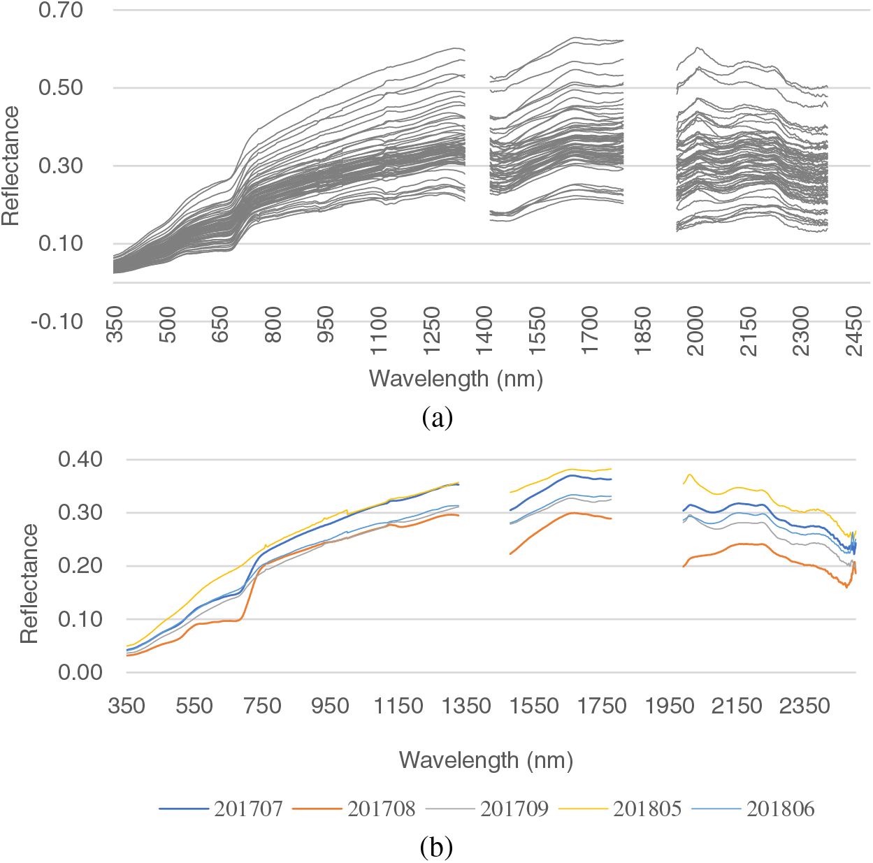
Figure 3: Original reflection spectrum curve. (a) Canopy reflectance curve of grassland in some sample plots; (b) Grassland canopy reflectance curve in different months

The canopy reflectance curves of the grassland after exclusion show the spectral patterns of green vegetation. However, the peaks and valleys of some curves are insignificant, which is caused by the variability in the composition of grass plant species, vegetation cover, and non-uniform grass growth. After eliminating the invalid spectral curves, the final grass canopy reflectance curves of different months were obtained (Fig. 3b).

The original spectral curves exhibit no green light reflection peaks and red light absorption peaks in May, June, and September. The plants were in the re-greening period in May and June. In September, they were disturbed by the mowing period and the bare soil, resulting in no significant spectral reflectance characteristics. In contrast, the spectral characteristics are significant in July and August due to the continuous growth of the grass community. During this period, new leaves kept growing, with increasing biomass and leaf area index. The increased photosynthetic capacity of the plant population and the promoted absorption of blue and red light gradually decreased the reflectance of blue and red light areas. The reflectance of the green light region formed a small reflection peak (green peak) and an absorption valley (red valley). With the increase of AGB and the leaf area index, the reflectance in the near-infrared region continuously increases, forming a wave peak at 675–760 nm with a significant and gentle change in reflectance. The reflectance decreases significantly in the near-infrared band between 1418 and 1530 nm, with an absorption valley near 1460 nm and an absorption peak near 1660 nm. In the shortwave infrared region, the reflectance continuously decreases until the stabilization of the grass community.

These results indicate that July and August are the best time to collect field data for remote sensing inversion of typical grasslands in Inner Mongolia. However, there are no significant reflection spectral features in May, June, and September due to the influence of soil and anthropogenic activities, leading to more uncertainties in remote sensing inversion.

3.1.2 Spectral Derivative Transformation Curves of Typical Grasslands in Different Periods

After the first-order derivative transformation of the original spectral reflectance, the “double peaks”, “red edge” and “blue edge” of the canopy spectrum appear in July and August (Fig. 4a), with a larger amplitude of the red edge and a smaller amplitude of the blue edge. However, the spectral curves in May, June, and September are affected by biomass and leaf area, and the “peaks” and “valleys” of reflectance in the visible and near-infrared regions are insignificant. These results suggest that the first-order derivative spectra can well eliminate the effect of soil background on the canopy spectra.

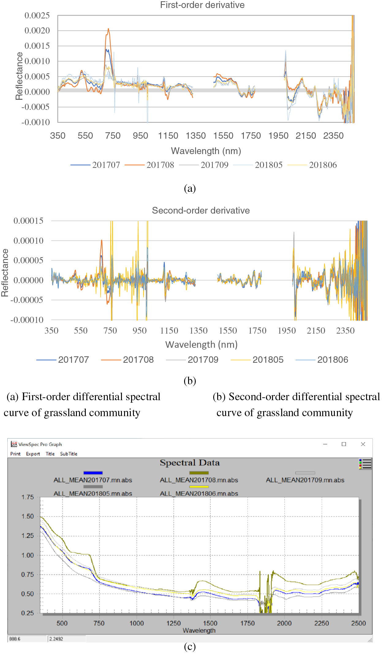
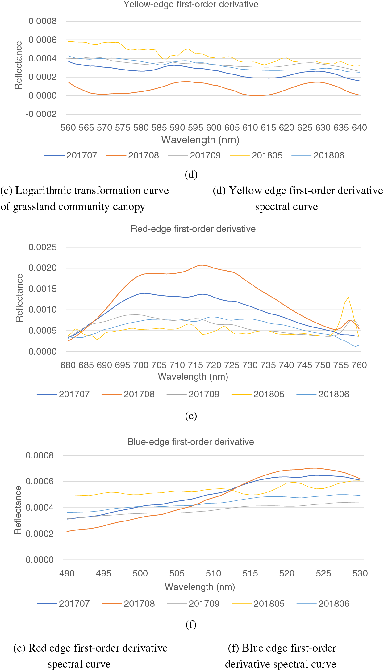
Figure 4: Canopy spectral derivative conversion curves and trilateral feature analysis images of typical grassland in different periods

The second-order differential transformed spectra curves show similar trends in July and August, with a significant difference at 719 nm. The changes in May, June, and September are basically the same, exhibiting no regular variations (Fig. 4b). The minor second-order differences in the reflectance of the grass canopy spectra suggest that the second-order derivative spectra can completely or largely eliminate the background noise spectrum. However, the actual field background spectra are more complex and can be eliminated using higher derivative spectra.

The logarithmic transformation enhances the variability of the spectral features in the visible region while reducing the influence of multiplicative factors due to different lighting conditions (Fig. 4c). In July and August, a clear peak is observed in the visible region for spectral reflectance, while no significant pattern occurs in the near-infrared region. It indicates that the reflectance amplitude in the visible region of the original spectrum is low. After spectral transformation, more significant amplitude differences occur in the visible region.

3.1.3 Trilateral Characteristics of Typical Grasslands in Different Periods

The parameters based on the spectral position mainly include “blue edge”, “yellow edge”, and “red edge” (called “trilateral”), reflecting important spectral features of the vegetation. The “red edge” refers to the transition region from red to near-infrared light, with wavelengths ranging from 680 to 760 nm and first-order derivatives. The “blue edge” refers to the transition region from blue to green light, with wavelengths ranging from 490 to 530 nm and first-order derivatives. The “yellow edge” refers to the transition zone between green and red lights, with wavelengths ranging from 560 to 640 nm and first-order derivatives. The first- and second-order derivatives for July and August were used to extract the grass spectral parameters, as shown in Fig. 4.

The first-order derivative spectral curves of the red edge show inconsistent trends in different periods (Fig. 4e). The spectral reflectance increases in July and August and decreases after reaching the peak, with “double peaks” at 701 and 717 nm. In addition, no significant changes were observed in June, July, and September. The reason may be that May and June are in the stages of grass growth with small plant canopy areas. The “double peak” phenomenon is insignificant due to the soil background. September is in the late stage of grass growth, at which the leaves begin to turn yellow and fall off, and the “double peak” phenomenon gradually diminishes. The first-order derivative spectra of the blue edge also show a trend of first increasing and then decreasing in July and August, with a significant peak at 524 nm (Fig. 4f). No significant changes were observed in June, July, and September. The first-order derivative spectra of the yellow edges show “double peaks” at 589 and 628 nm in July and at 593 and 628 nm in August (Fig. 4d). No significant changes are observed in June, July, and September.

3.1.4 Correlation Analysis of Biomass and Reflectance

As shown in Fig. 5, dry biomass and vegetation canopy reflectance negatively correlated with the 350–716 nm band, with a correlation coefficient of −0.441 at 678 nm. A positive correlation was observed on the 717–1350 nm band, and a plateau appeared on the 744–966 nm band. All correlation coefficients were above 0.25, with an average of 0.291 and a maximum value of 0.302 at 887 nm. Two peaks appeared on the 967–1350 band, with correlation coefficients of 0.324 at 1090 nm and 0.332 at 1291 nm, respectively. A negative correlation was observed on the 1421–1601 nm band, with the minimum correlation coefficient of −0.140 at 1460 nm. A positive correlation was observed on the 1602–1800 nm band, with the maximum correlation coefficient of 0.188 at 1661 nm. A negative correlation was observed on the 1951–2350 nm band.

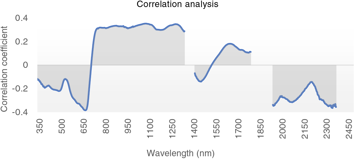
Figure 5: Correlation coefficient between dry AGB and grassland canopy spectra

The minimum negative correlation coefficient appeared at 678 nm in the red band, and the maximum positive correlation coefficient appeared at 887 nm in the NIR band.

3.2 The Estimation Model of the Ground Spectrum and UAV Imaging Spectrum Was Constructed

3.2.1 Analysis of Resonon Hyperspectral Data and Grassland Canopy Spectral Characteristics

As shown in Fig. 6a, figure shows the spectral reflectance curves of grassland canopy collected by ground-based ASD and UAV remote sensing, where the trends of hyperspectral information are generally consistent. However, the UAV data are slightly higher than the ASD on the green light band. The different geometric positions of the target, sensor, and sun for the two remote sensing platforms result in different reflectance distribution functions in both directions. Research has demonstrated that the bidirectional reflectance distribution function significantly affects low-altitude UAV data. Furthermore, different spectral response functions may also cause differences.

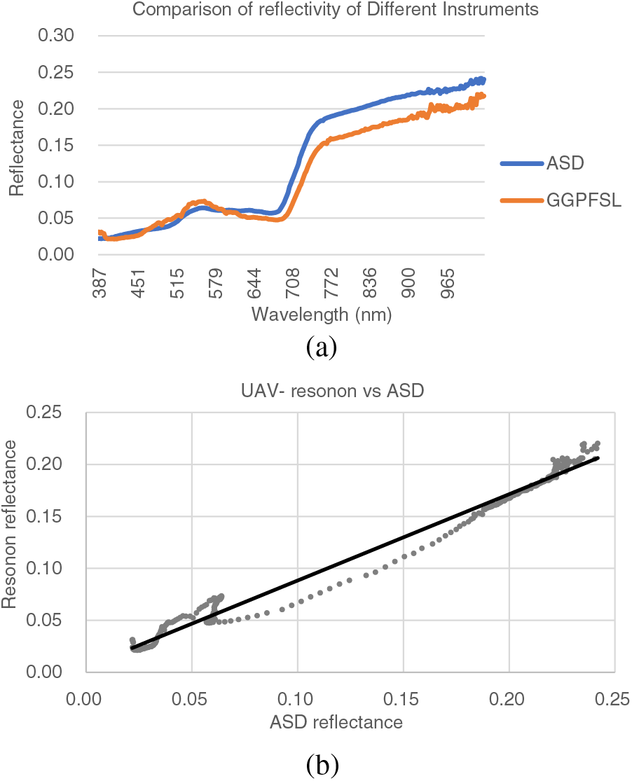
Figure 6: Comparison of ASD and UAV spectral reflectance analyses. (a) Original spectral reflectance curve of grassland canopy with the two instruments; (b) Reflectance comparison between ASD and Resonon hyperspectral data

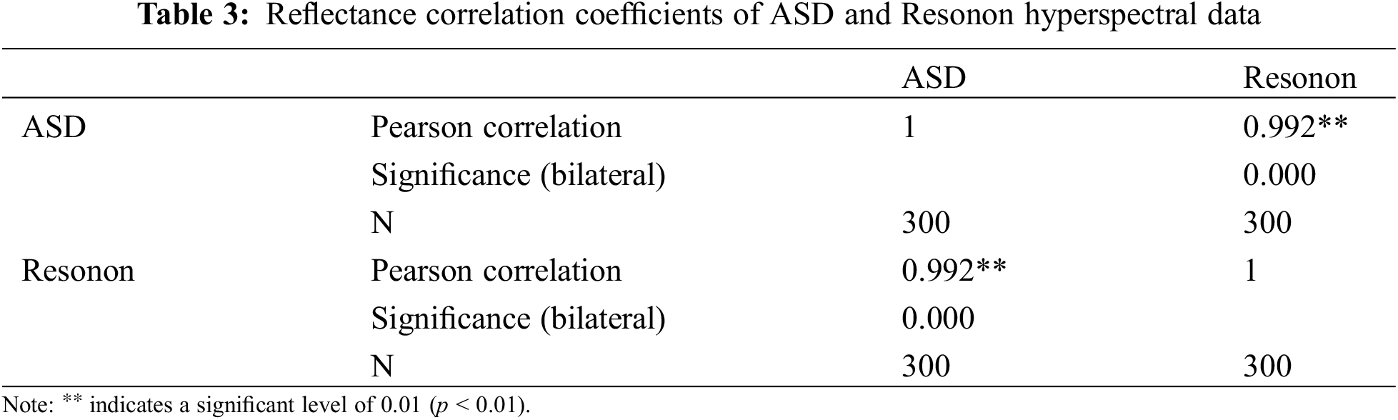
Comparison between the UAV Resonon hyperspectral data and the ground-based ASD spectral reflectance of grassland canopy suggested a significant correlation between the two sensor spectral data (Fig. 6b). This result was verified by Pearson correlation analysis, with correlation coefficients of 0.99 or above, the results were shown in Table 3.

3.2.2 Sensitive Band Selection

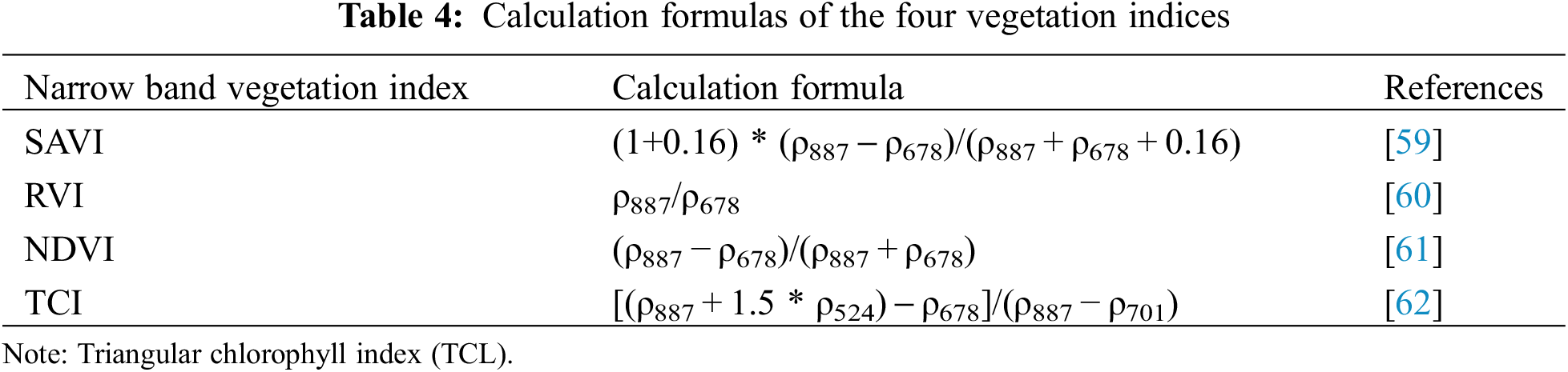
Sensitive bands were screened by ASD grassland canopy spectral analysis and hyperspectral feature correlation analysis. The red edge band was 701 nm, the blue edge band was 524 nm, the red light band was 678 nm, and the NIR band was 887 nm. On this basis, the narrow-band vegetation index was calculated. In the three-edge feature analysis, significant peaks were observed at 701 nm on the red edge and 524 nm on the blue edge. In the correlation analysis between biomass and raw spectra, the minimum negative correlation coefficient was observed at 678 nm, and the maximum positive correlation coefficient was observed at 887 nm. Based on the sensitive bands, four vegetation indices were selected for hyperspectral yield estimation in this study. The establishment of vegetation index was shown in Table 4.

3.2.3 Correlation Analysis of ASD/Resonon Data and AGB Dry/Fresh Weights

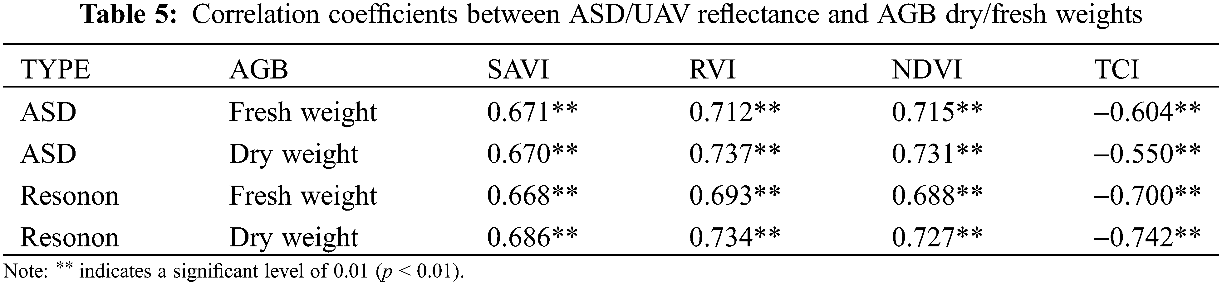
The following results were obtained from the correlation analysis (Table 5). A significant correlation was obtained between grassland biomass and vegetation indices extracted from ASD and Resonon data. Regarding the ASD reflectance-based vegetation indices, the fresh weight of aboveground standing biomass showed the strongest correlation with NDVI, with a correlation coefficient of 0.715. The dry weight of aboveground standing biomass exhibited the strongest correlation with RVI, with a correlation coefficient of 0.737. In terms of the vegetation indices extracted from the Resonon data, SAVI, RVI, and NDVI were positively correlated with the aboveground fresh/dry biomass, with RVI having the largest correlation coefficients of 0.693 and 0.734. TCI showed negative correlations with the aboveground fresh/dry biomass, with correlation coefficients of −0.700 and −0.742.

3.2.4 Estimation Models of ASD/Resonon Data with AGB Dry/Fresh Weights

The GLM model was used to develop the best-fit model. The results showed that the goodness of fitting between ASD canopy reflectance-based vegetation indices and AGB fresh weight was NDVI > RVI > SAVI > TCI. The exponential model constructed with NDVI as the independent variable had the highest R2 of 0.549. The goodness of fitting between ASD canopy reflectance-based vegetation indices and AGB dry weight was RVI > NDVI > SAVI > TCI. The exponential model constructed with RVI as the independent variable had the highest R2 of 0.587 (Table 6). After the model accuracy validation, the following results were obtained. ASD canopy reflectance-based vegetation indices and AGB dry/fresh weights exhibited strong correlations. The validation models selected the model with the highest fitting R2 and prediction R2 for ASD hyperspectral estimation of AGB dry/fresh weight. According to the comparative analysis between the measured and predicted fresh weight of aboveground standing biomass based on the four vegetation index models, the optimal performance ranked as SAVI > NDVI > RVI > TCI (Fig. 7).

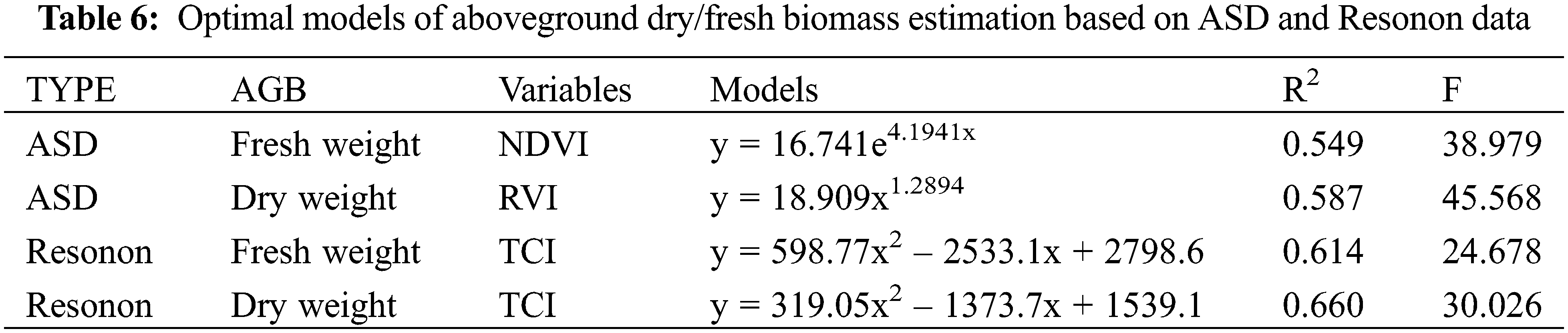
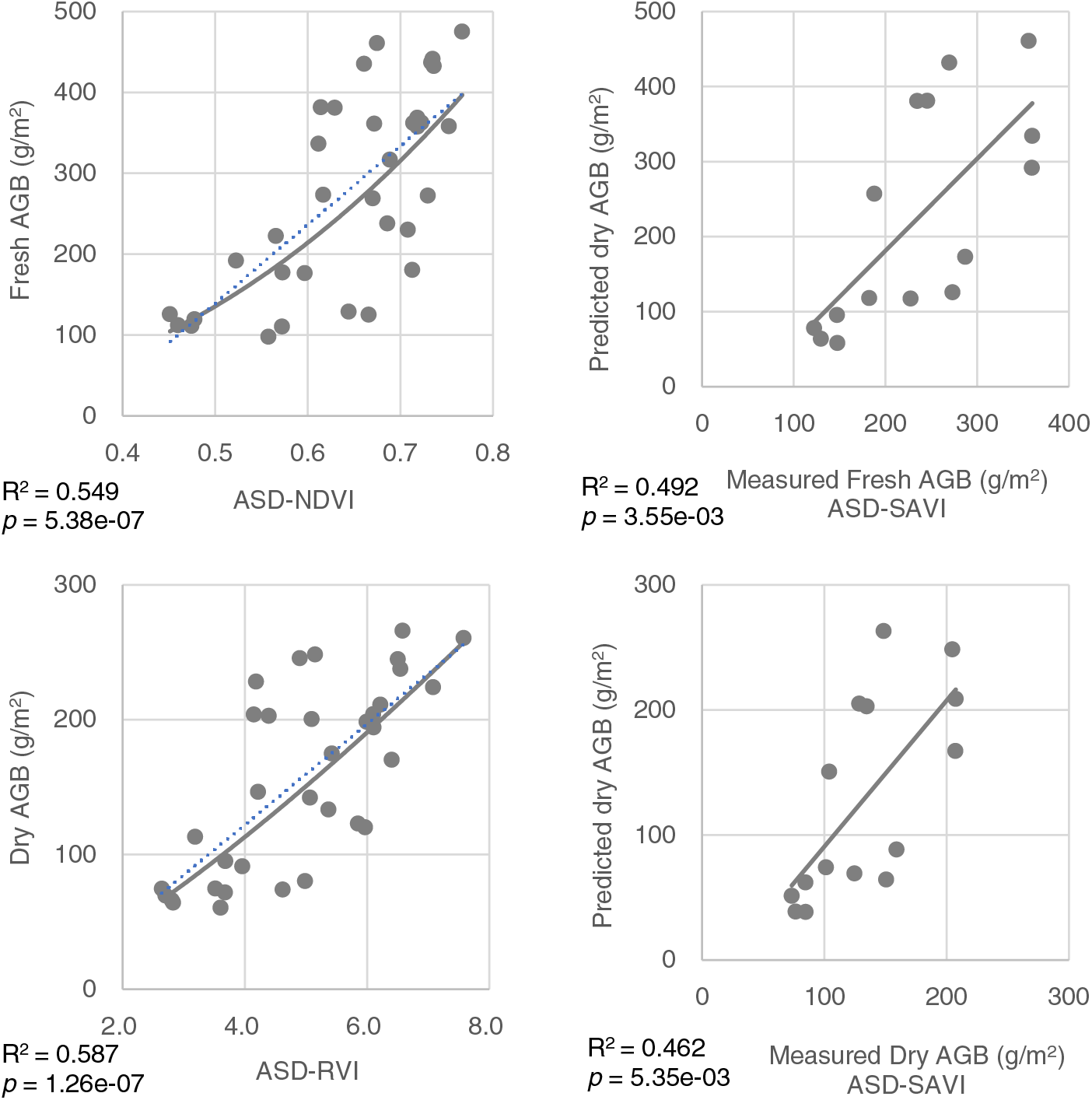
Figure 7: Optimal fitting model and validation model of dry/fresh AGB and ASD canopy reflectance

According to the previous section, the Resonon hyperspectral vegetation indices significantly correlated with AGB dry/fresh weights. On this basis, the AGB dry/fresh weight GLM fitting model was established. The results showed that the goodness of fitting between the four Resonon data-based vegetation indices and AGB fresh weights was TCI > RVI > NDVI > SAVI. Among them, the quadratic function model with TCI as the independent variable was optimal, with an R2 of 0.614. The goodness of fitting of the GLM models built with the four vegetation indices and AGB dry weight was TCI > RVI > NDVI > SAVI. The optimal model fitted with the TCI vegetation index was a quadratic model with an R2 of 0.660. This result was consistent with the fitting results of AGB fresh weight. The following results were obtained from model validation. The model with the highest fitting R2 and prediction R was selected for Resonon hyperspectral estimation of AGB fresh weight. According to the comparative analysis between the measured and predicted dry weight of aboveground standing biomass based on the four vegetation index models, the optimal performance was SAVI > RVI > EDVI > TCI (Fig. 8).

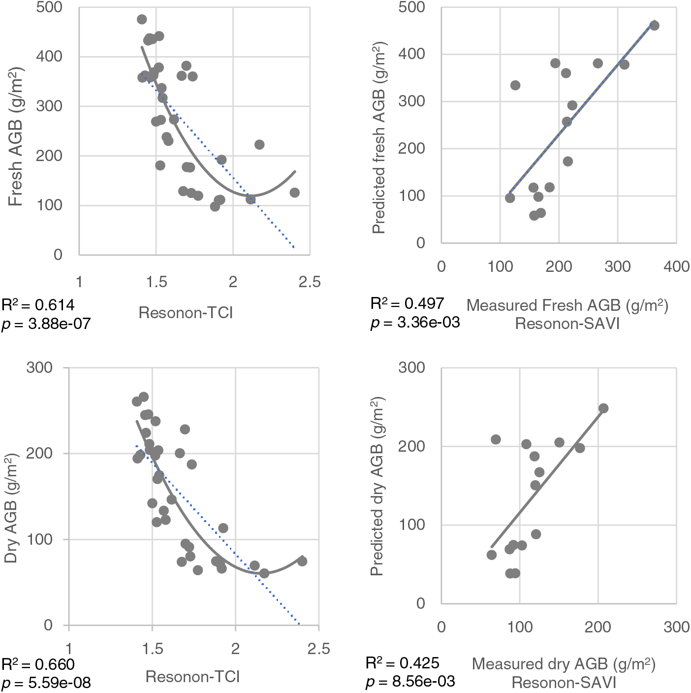
Figure 8: Best fit model and validation model of dry/fresh AGB and resonon reflectance data

According to the modeling analysis between ASD/Resonon hyperspectral data and AGB fresh/dry weights, SAVI, NDVI, RVI, and TCI were significantly correlated with aboveground standing biomass. Regression analysis was conducted based on the data of 54 sample points collected in the field (excluding 5 outliers), and the estimation model was established, where the number of test samples was 34 and 15, respectively. According to the comparison between the fitted and predicted results, the best inversion models in all generalized linear simulations of aboveground standing biomass were those with SAVI as the variable:

(1) Resonon data with AGB fresh weight: y = 33.952e4.526x, with the fitting R2 of 0.488, the prediction R2 of 0.449, and the RMSE and REE of 105.75 and 0.62, respectively.

(2) Resonon data with AGB dry weight: y = 17.962e4.672x, with the fitting R2 of 0.542, the prediction R2 of 0.424, and the RMSE and REE of 57.03 and 0.65, respectively.

(3) ASD hyperspectral data with AGB fresh weight: y = 1203.5x2.0469, with the fitting R2 of 0.474, the prediction R2 of 0.412, and the RMSE and REE of 123.28 and 0.53, respectively.

(4) ASD hyperspectral data with AGB dry weight: y = 16.468e4.5684x, with the fitting R2 of 0.461, the prediction R2 of 0.461, and the RMSE and REE of 104.63 and 0.79, respectively.

Among all variables, SAVI was the best, making it suitable for hyperspectral remote sensing inversion modeling of typical grasslands in Inner Mongolia. The best SAVI model was used to invert the dry weight distribution of AGB, and the results were shown in Fig. 9.

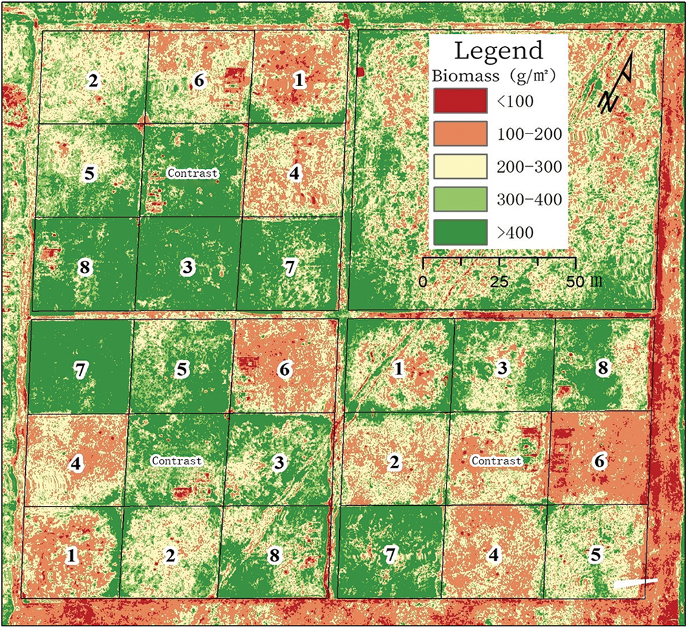
Figure 9: Spatial distribution of dry AGB predicted by SAVI based on the resonon data

4  Discussion

4.1 Mixed Spectral Analysis of Grassland Canopy

The spectral reflectance of grassland canopy is a mixed spectrum, and its complexity depends on factors such as vegetation type, vegetation coverage, growth period, atmosphere, and soil background [63]. In the visible region, plant chlorophyll was an important factor affecting reflectivity. As shown in Fig. 3a, the spectral curve shows a “steep slope” shape in the red edge region of 675–760 nm, indicating that the spectral characteristics are closely related to the biophysical parameters of grassland. During the growth and development period of grassland, significant spectral characteristics of vegetation were observed in July and August, while the plants in May and June were affected by the re-greening period. The influence of the weeding period in September and the interference of the soil background resulted in no significant spectral reflection characteristics on the spectral curve. After the derivative transformation of the original spectrum, a significant “double peak” phenomenon was observed in July and August on the first-order differential curve, accompanied by “red edge” and “blue edge” phenomena. However, the red edge radiation value was larger, and the blue edge radiation value was smaller, suggesting that the first-order derivative spectrum of the grassland community canopy can well eliminate the influence of soil background. As shown in Fig. 4b, the spectral curves of July and August after the second-order differential transformation are close in the spectral range, indicating that the second-order derivative spectrum can completely or basically eliminate the background noise. The logarithmic transformation can enhance the difference of spectral characteristics in the visible region, but no significant rule was observed in the near-infrared region.

“Red edge” is an important parameter to characterize the chlorophyll content of vegetation and a critical index to describe the health status of vegetation [64]. The “red edge” phenomenon refers to the strong absorption of visible light in the red band by vegetation chlorophyll, and the “vegetation climbing” phenomenon appears in the spectral range of the strong reflection near-infrared band (about 680–750 nm). It is the most significant spectral feature that distinguishes green vegetation from other ground objects, and it is also the “inflection point” of the first derivative of hyperspectral in this interval. Tang et al. [65] identified a significant correlation between hyperspectral “red edge” parameters and rice aboveground fresh/dry biomass and leaf area index. Feng et al. [66] established models for estimating winter wheat yield using a single vegetation index and a combination of the vegetation index and red edge parameters. The results showed that the combination of the vegetation index and red edge parameters achieved improved yield estimation compared to using the vegetation index alone. This result further validated the importance of the “red edge” parameter in extracting hyperspectral features. This study conducted the derivative transformation and hyperspectral characteristic variable correlation analysis of the grassland canopy spectrum. Based on the analysis results, the sensitive bands were selected. The red edge band was 701 nm, the blue edge band was 524 nm, the red light band was 678 nm, and the near-infrared band was 887 nm.

4.2 Analysis of Model Inversion Accuracy

Compared with traditional multispectral remote sensing data, hyperspectral remote sensing data exhibit higher spectral resolution and more spectral information, enabling the identification of many problems that cannot be solved by multispectral broadband studies. However, due to a large number of hyperspectral data and high band dimensions, the full-band inversion model is unstable with low accuracy. The selection of sensitive bands and their optimal combinations are the keys to the accuracy of the fitting model. Yang et al. [67] proposed a sensitive band of nitrogen concentration in potato plants by band optimization algorithm in the field test areas of Siziwang Banner and Wuchuan County, Inner Mongolia. The blue-violet light in the band range of 400–450 nm and the red edge band in the band range of 690–720 nm were used to establish the vegetation index to estimate the nitrogen concentration of potato plants, which improved the index sensitivity in the diagnosis of high nitrogen concentration. Zhang et al. [68] used the continuous projection algorithm and the regression coefficient method to extract the 690–720 nm spectral information of the visible and near-infrared bands. The sensitive bands of rape at different growth stages were obtained. Kim et al. [69] monitored the corn canopy nitrogen fertilizer experimental field by hyperspectral technology. The results showed that the more sensitive bands were 800, 650, and 550 nm. As shown in Table 4, the vegetation index constructed by ASD non-imaging hyperspectral data and UAV imaging hyperspectral data was significantly correlated with AGB fresh/dry weight. The estimation model integrates ground hyperspectral and UAV imaging spectrometer data. The comparison between fitting R2 and verifying R2 shows that the AGB in dry weight form fits the inversion model better. The UAV imaging hyperspectral shows better goodness of fitting with the AGB estimation model. Li et al. [29] used low-altitude UAVs to measure the spectra of potatoes at different growth stages. The two narrow-band vegetation indices selected by the characteristic bands were combined to predict the AGB. Taking the typical desert shrub area in Inner Mongolia as an example, Peng et al. [26] developed an improved method and used UAV RGB (red, green, and blue) images to simultaneously extract three feature metrics to estimate AGB. Mowll et al. [70] used a combination of UAV-derived data sets to generate a vegetation index and micro-terrain model. A random forest algorithm was adopted to estimate grassland AGB, and a more accurate estimation model was obtained.

In this study, four (NDVI, RVI, TCI, SAVI) vegetation indices of ground and airborne hyperspectral were calculated based on sensitive bands, and the AGB inversion models of typical grasslands in Inner Mongolia were established, respectively, and the model results showed that the nonlinear fitting accuracies of the four vegetation index models were higher than that of the linear fitting, which indicated that the four index-fitting models were affected by different degrees of supersaturation problems [71]. By comparing the fitting R2 it was found that the TCI and RVI vegetation index construction models had better accuracy, but comparing the fitting results of the inversion models with the measured results, the SAVI model validation R2 was 0.424, and the NDVI model validation R2 was 0.353, which improved the estimation accuracy by 20%, and compared with TCI and RVI, the estimation accuracies were improved by 46% and 14%, respectively. Therefore, the SAVI vegetation index model was finally found to be the optimal AGB inversion model were the best. This is consistent with the findings of many scholars (Zhang et al. [72], Zhen et al. [73]). Compared with the NDVI index, the SAVI index introduces a soil adjustment factor L, which further reduces the effect of soil background changes on the vegetation index, and also reduces the effect of insufficient accuracy of the inversion model caused by the easy saturation of the NDVI index in areas with high vegetation cover.

4.3 Discussion on Uncertainty Factors of Remote Sensing Inversion

Grassland biomass inversion using remote sensing faces many uncertainties. Some potential improvements are summarized as follows. (1) There are uncertainties in remote sensing image acquisition. Different remote sensing platforms and the physical parameters of the sensors can result in differences in obtained remote sensing data. (2) The spatial resolution refers to the size of the actual ground area represented by each image element on the remote sensing image. For example, the MODIS 1,2 band image element area is 250 m × 250 m. Regardless of size, only one DN value was recorded for each image element. In the case of small and diverse surface biomass classes, a higher spatial resolution allows for the acquisition of cleaner image elements. Considering the diverse grassland types in northern China, remote sensing images with low spatial resolution can hardly meet the accuracy requirements, and the rapid acquisition of high spatial resolution data has become a challenging problem. (3) The band location, bandwidth, and spectral response function of different sensors jointly determine the amount of radiation energy acquired on a sensor band. Therefore, using sensors with different parameters for ground biomass monitoring inevitably leads to uncertainties due to the different resolutions of the sensor spectra. (4) Uncertainties can be caused by radiometric calibration and atmospheric correction. Therefore, what was observed by different remote data sources is only one aspect.

The modeling method in this study was five GLM functions, which was relatively simple, and the model fitting accuracy was influenced by sample data quantity and quality. In contrast, machine learning and deep learning algorithms with higher fault tolerance can help solve the non-vulnerable fitting problem. Therefore, methods such as artificial neural networks and random forests will be considered in future research to improve model accuracy [74]. Furthermore, to improve the accuracy of grassland biomass inversion models, more influencing factors should be considered to improve vegetation index methods and establish more representative feature variables when extracting hyperspectral feature variables and selecting vegetation indices. Moreover, some studies showed that combining laser technology, microwave sensor technology, and optical remote sensing can effectively improve inversion accuracy [75]. These features will be considered in our future studies.

5  Conclusion

This study integrated ground-based hyperspectral and airborne hyperspectral data for remote sensing inversion of typical grassland biomass in Inner Mongolia. Sensitive bands were screened by ASD grassland canopy spectral analysis and hyperspectral feature correlation analysis. As a result, four hyperspectral vegetation indices, SAVI, NDVI, RVI, and TCI, were established. By analyzing the goodness of fitting between ground/airborne hyperspectral vegetation indices and aboveground standing biomass (fresh/dry weight), the model with SAVI as the independent variable was the best. The exponential equation for UAV hyperspectral data and the dry weight of aboveground standing biomass had the best fitting result, where y = 17.962e4.672x, the fitting R2 was 0.542, the prediction R2 was 0.424, and the RMSE and REE were 57.03 and 0.65, respectively.

The accuracy of estimating grassland AGB through inversion from multi-source remote sensing data depends on the spectral characteristics of the grassland canopy, the selection of data sources, multi-source data fusion, etc. These aspects were important development directions for remote sensing-based grassland biomass inversion in the future.

Acknowledgement: We acknowledge editors and reviewers for their positive and constructive comments and suggestions. Thank the grassland ecology research base of Inner Mongolia University for providing experimental sites.

Funding Statement: This study was supported by the Basic Research Business Fee Project of Universities Directly under the Inner Mongolia Autonomous Region (JY20220108), the Inner Mongolia Autonomous Region Natural Science Foundation Project (2022LHMS03006), the Inner Mongolia University of Technology Doctoral Research Initiation Fund Project (DC2300001284), and the Inner Mongolia Autonomous Region Natural Science Foundation Project (2021MS03082).

Author Contributions: Wang Ruochen drafted and revised the manuscript. Wang Xiumei proposed the concept of this study and reviewed the manuscript. Dong Jianjun conducted on-site experiments and collected image data. Jin Lishan and Sun Yuyan completed subsequent experiments. Wang Ruochen, Wang Xiumei, and Dong Jianjun analyzed and interpreted the results. Taogetao Baoyin reviewed the completed manuscript and provided good suggestions during the manuscript revision stage. All authors have read and approved the final manuscript.

Availability of Data and Materials: The datasets analysed during the current study are available from the corresponding author on reasonable request.

Ethics Approval: Not applicable.

Conflicts of Interest: The authors declare that they have no conflicts of interest to report regarding the present study.

References

1. Yang Y, Wang J, Chen Y, Cheng F, Liu G, He Z. Remote-sensing monitoring of grassland degradation based on the GDI in Shangri-La. Remote Sens. 2019;11(24):3030. [Google Scholar]

2. Lyu X, Li X, Gong J, Li S, Dou H, Dang D, et al. Remote-sensing inversion method for aboveground biomass of typical steppe in Inner Mongolia. Ecol Indic. 2021;120:106883. [Google Scholar]

3. Conant RT, Cerri CE, Osborne BB, Paustian K. Grassland management impacts on soil carbon stocks: a new synthesis. Ecol Appl. 2017;27(2):662–8. [Google Scholar] [PubMed]

4. Huang W, Li W, Xu J, Ma X, Li C, Liu C. Hyperspectral monitoring driven by machine learning methods for grassland above-ground biomass. Remote Sens. 2022;14(9):2086. [Google Scholar]

5. Zhang X, Niu J, Buyantuev A, Zhang Q, Dong J, Kang S, et al. Understanding grassland degradation and restoration from the perspective of ecosystem services: a case study of the Xilin River Basin in Inner Mongolia. Sustain. 2016;8(7):594. [Google Scholar]

6. Wijesingha J, Astor T, Schulze-Brüninghoff D, Wengert M, Wachendorf M. Predicting forage quality of grasslands using UAV-borne imaging spectroscopy. Remote Sens. 2020;12(1):126. [Google Scholar]

7. Bao N, Li W, Gu X, Liu Y. Biomass estimation for semiarid vegetation and mine rehabilitation using worldview-3 and sentinel-1 SAR imagery. Remote Sens. 2019;11(23):2855. [Google Scholar]

8. Batistoti J, Marcato-Junior J, Ítavo L, Matsubara E, Gomes E, Oliveira B, et al. Estimating pasture biomass and canopy height in Brazilian savanna using UAV photogrammetry. Remote Sens. 2019;11(20):2447. [Google Scholar]

9. Kong B, Yu H, Du R, Wang Q. Quantitative estimation of biomass of alpine grasslands using hyperspectral remote sensing. Rangeland Ecol Manag. 2019;72(2):336–46. [Google Scholar]

10. Yue J, Feng H, Jin X, Yuan H, Li Z, Zhou C, et al. A comparison of crop parameters estimation using images from UAV-mounted snapshot hyperspectral sensor and high-definition digital camera. Remote Sens. 2018;10(7):1138. [Google Scholar]

11. Zhou X, Zheng HB, Xu XQ, He JY, Ge XK, Yao X, et al. Predicting grain yield in rice using multi-temporal vegetation indices from UAV-based multispectral and digital imagery. ISPRS J Photogramm. 2017;130:246–55. [Google Scholar]

12. Tao H, Feng H, Xu L, Miao M, Long H, Yue J, et al. Estimation of crop growth parameters using UAV-based hyperspectral remote sensing data. Sens. 2020;20(5):1296. [Google Scholar]

13. Liang B, Liu X, Hao Y, Chu B, Tang Z. Extraction of vegetation biomass in desert areas based on 5 vegetation indices. Res Arid Areas. 2023;40(4):647–54 (In Chinese). [Google Scholar]

14. Zhao F, Xu B, Yang X, Jin Y, Li J, Xia L, et al. Remote sensing estimates of grassland aboveground biomass based on MODIS net primary productivity (NPPa case study in the Xilingol grassland of Northern China. Remote Sens. 2014;6(6):5368–86. [Google Scholar]

15. Liang T, Yang S, Feng Q, Liu B, Zhang R, Huang X, et al. Multi-factor modeling of above-ground biomass in alpine grassland: a case study in the three-river headwaters region. Remote Sens Environ. 2016;186:164–72. [Google Scholar]

16. John R, Chen J, Giannico V, Park H, Xiao J, Shirkey G, et al. Grassland canopy cover and aboveground biomass in Mongolia and Inner Mongolia: spatiotemporal estimates and controlling factors. Remote Sens Environ. 2018;213:34–48. [Google Scholar]

17. Wang P, Wan R, Yang G. Research progress on wetland plant classification and biomass inversion based on multi-source remote sensing data. Wetland Sci. 2017;15(1):114 (In Chinese). [Google Scholar]

18. Liu YN. Research on estimating aboveground biomass and net primary productivity of forests based on multi-source remote sensing data. J Surveying Mapp. 2020;49(12):1641. [Google Scholar]

19. Feng R, Zhang Y, Wu JW, Ji RP, Yu WY, Wang PJ. Research progress on drought remote sensing monitoring based on multispectral and hyperspectral data. Disaster Sci. 2019;34(1):162–6 (In Chinese). [Google Scholar]

20. Fernández-Habas J, Cañada MC, Moreno AMG, Leal-Murillo JR, Gonzalez-Dugo MP, Oar B, et al. Estimating pasture quality of Mediterranean grasslands using hyperspectral narrow bands from field spectroscopy by random forest and PLS regressions. Comput Electron Agric. 2022;192:106614. [Google Scholar]

21. Wang Z, Ma Y, Zhang Y, Shang J. Review of remote sensing applications in grassland monitoring. Remote Sens. 2022;14(12):2903. [Google Scholar]

22. Zhang FH, Huang MX, Zhang J, Bao G, Bao YH. A study on using hyperspectral identification of grassland species–taking the Xilingol grassland as an example. Surveying Mapp Bull. 2014;7:66–9 (In Chinese). [Google Scholar]

23. Ulan Tuya, Bao G, Wu Y, Huang MX, Hang YL, Bao YH. Research on hyperspectral remote sensing estimation of aboveground biomass in grasslands. J Inner Mongolia Norm Univ (Natural Sci Chin Edition). 2015;5:660–6 (In Chinese). [Google Scholar]

24. Cao Y, Jiang K, Wu J, Yu F, Du W, Xu T. Inversion modeling of japonica rice canopy chlorophyll content with UAV hyperspectral remote sensing. PLos One. 2020;15(9):e0238530. [Google Scholar]

25. Song QJ, Cui X, Zhang YY, Meng BP, Gao JL, Xiang YX. Research on grassland vegetation coverage based on small unmanned aerial vehicles and modis data–taking gannan prefecture as an example. Grassl Sci. 2017;34(1):40–50 (In Chinese). [Google Scholar]

26. Mao P, Qin L, Hao M, Zhao W, Luo J, Qiu X, et al. An improved approach to estimate above-ground volume and biomass of desert shrub communities based on UAV RGB images. Ecol Indic. 2021;125:107494. [Google Scholar]

27. Peciña MV, Bergamo TF, Ward RD, Joyce CB, Sepp K. A novel UAV-based approach for biomass prediction and grassland structure assessment in coastal meadows. Ecol Indic. 2021;122:107227. [Google Scholar]

28. Yang W, Nigon T, Hao Z, Paiao GD, Fernández FG, Mulla D, et al. Estimation of corn yield based on hyperspectral imagery and convolutional neural network. Comput Electron Agric. 2021;184:106092. [Google Scholar]

29. Li B, Xu X, Zhang L, Han J, Bian C, Li G, et al. Above-ground biomass estimation and yield prediction in potato by using UAV-based RGB and hyperspectral imaging. ISPRS J Photogramm. 2020;162:161–72. [Google Scholar]

30. Wengert M, Wijesingha J, Schulze-Brüninghoff D, Wachendorf M, Astor T. Multisite and multitemporal grassland yield estimation using UAV-borne hyperspectral data. Remote Sens. 2022;14(9):2068. [Google Scholar]

31. Liu X, Wang H, Cao Y, Yang Y, Sun X, Sun K, et al. Comprehensive growth index monitoring of desert steppe grassland vegetation based on UAV hyperspectral. Front Plant Sci. 2023;13:1050999. [Google Scholar] [PubMed]

32. Fu S, Zhang YH, Li JL, Wang ZM, PL, Feng QS. The impact of different vegetation indices and drone altitude on the accuracy of grassland coverage estimation. Grassl Sci. 2021;38(1):11–9 (In Chinese). [Google Scholar]

33. Xu C, Liu W, Zhao D, Hao Y, Xia A, Yan N, et al. Remote sensing-based spatiotemporal distribution of grassland aboveground biomass and its response to climate change in the Hindu Kush Himalayan Region. Chinese Geogr Sci. 2022;32(5):759–75 (In Chinese). [Google Scholar]

34. Rajakumari S, Mahesh R, Sarunjith KJ, Ramesh R. Building spectral catalogue for salt marsh vegetation, hyperspectral and multispectral remote sensing. Reg Stud Mar Sci. 2022;53:102435. [Google Scholar]

35. Zhao YH, Hou P, Jiang JB, Jiang Y, Zhang B, Bai JJ, et al. Progress in quantitative inversion research methods for vegetation ecological remote sensing parameters. J Rem Sens. 2021;25(11):2173–97. [Google Scholar]

36. Darvishzadeh R. Hyperspectral remote sensing of vegetation parameters using statistical and physical models. ITC Dissertation. 2008;152:2–8. [Google Scholar]

37. Cai QK. Hyperspectral remote sensing inversion of winter wheat leaf area index and chlorophyll content. China: Water Resources and Hydropower Publishing House; 2019. p. 2–3 (In Chinese). [Google Scholar]

38. Yang PW, Fu G, Li YL, Zhou YT, Shen ZX. Estimating aboveground biomass of alpine grasslands in northern Tibet using multispectral cameras. Grassl Sci. 2014;7:1211–7 (In Chinese). [Google Scholar]

39. Huete AR. A soil-adjusted vegetation index (SAVI). Remote Sens Environ. 1988;25(3):295–309. [Google Scholar]

40. Liu ZY, Huang JF, Wang FM, Wang Y. Adjusted normalized vegetation index for estimating rice leaf area index. Chin Agric Sci. 2008;41(10):3350–6 (In Chinese). [Google Scholar]

41. Gao ML, Zhao WJ, Gong ZN, He XH. Inversion of vegetation biomass in the Yellow River wetland based on environmental satellite data. J Ecol. 2013;33(2):542–53. [Google Scholar]

42. Lyu X, Li X, Gong J, Wang H, Dang D, Dou H, et al. Comprehensive grassland degradation monitoring by remote sensing in Xilinhot, Inner Mongolia. China Sustain. 2020;12(9):3682. [Google Scholar]

43. Yan M, Zuo HJ, Zhang Y. The characteristics of the rejuvenation of Stipa grandis on the Xilinhot grassland and its relationship with meteorological factors. J Ecol Environ. 2019;28(7):1307–12. [Google Scholar]

44. Karakoc A, Karabulut M. Ratio-based vegetation indices for biomass estimation depending on grassland characteristics. Turk J Bot. 2019;43(5):619–33. [Google Scholar]

45. Kong JX, Zhang ZC, Zhang J. Plant species classification and identification based on multi-source remote sensing data: research progress and prospects. Biodivers. 2019;27(7):796. [Google Scholar]

46. Pfitzner K, Bartolo R, Whiteside T, Loewensteiner D, Esparon A. Multi-temporal spectral reflectance of tropical savanna understorey species and implications for hyperspectral remote sensing. Int J Appl Earth Observ Geoinform. 2022;112:102870. [Google Scholar]

47. Chen C, Du JM, Yang HY. Extraction and analysis of hyperspectral characteristics of vegetation in desertified grasslands of Inner Mongolia. Opt Instru. 2018;40(6):42–7 (In Chinese). [Google Scholar]

48. Gao S, Lin J, Ma T, Wu JG, Zheng JH. Spectral feature extraction and analysis of Artemisia annua on the Bayinbuluke grassland in Xinjiang. Remote Sens Technol Appl. 2018;33(5):908–14 (In Chinese). [Google Scholar]

49. Tsai F, Philpot W. Derivative analysis of hyperspectral data. Remote Sens Environ. 1998;66(1):41–51. [Google Scholar]

50. Huang JF, Wang FM, Wang XZ. Experimental study on rice hyperspectral remote sensing. China: Zhejiang University Press; 2010. p. 1–2 (In Chinese). [Google Scholar]

51. Alckmin GT, Lucieer A, Rawnsley R, Kooistra L. Perennial ryegrass biomass retrieval through multispectral UAV data. Comput Electron Agric. 2022;193:106574. [Google Scholar]

52. Liu Y, Feng H, Yue J, Li Z, Jin X, Fan Y, et al. Estimation of aboveground biomass of potatoes based on characteristic variables extracted from UAV hyperspectral imagery. Remote Sens. 2022;14(20):5121. [Google Scholar]

53. Chen Q, Yang J, Yan R, Li N, Jia Z. Analysis of NDVI Variation characteristics of different vegetation types in desert areas—A case study of alxa league. Chin J Grassl. 2022;44:17–28 (In Chinese). [Google Scholar]

54. Matese A, Berton A, Chiarello V, Dainelli R, Nati C, Pastonchi L, et al. Determination of riparian vegetation biomass from an unmanned aerial vehicle (UAV). For. 2021;12(11):1566. [Google Scholar]

55. Liu Y, Feng H, Yue J, Fan Y, Jin X, Zhao Y, et al. Estimation of potato above-ground biomass using UAV-based hyperspectral images and machine-learning regression. Remote Sens. 2022;14(21):5449. [Google Scholar]

56. Jacon AD, Galvao LS, Dalagnol R, dos Santos JR. Aboveground biomass estimates over Brazilian savannas using hyperspectral metrics and machine learning models: experiences with Hyperion/EO-1. Gisci Remote Sens. 2021;58(7):1112–29. [Google Scholar]

57. Yi Q, Huang JF, Wang XZ, Qian Y. Research on Hyperspectral remote sensing estimation model for corn chlorophyll. Sci Technol Bull. 2007;23(1):83–7 (In Chinese). [Google Scholar]

58. Zhang S, Bai Y, Liu Q, Tong DM, Xu ZT, Zhao N, et al. Estimating winter wheat yield in Shandong Province using remote sensing vegetation index and CASA model. Spectrosc Spect Anal. 2021;41(1):257–64 (In Chinese). [Google Scholar]

59. Dong QL, Lin H, Sun H, Qiu L, Zhang Y. Applicability of multi-source remote sensing data fusion method in wetland classification. J Cent South Univ For Technol. 2013;(1):52–7 (In Chinese). [Google Scholar]

60. Gao XL, Wang XQ. The application of multi-source remote sensing data in vegetation identification and extraction. Resour Sci. 2008;(1):153–8 (In Chinese). [Google Scholar]

61. Crasto N, Hopkinson C, Forbes DL, Lesack L, Marsh P, Spooner I, et al. A LiDAR-based decision-tree classification of open water surfaces in an Arctic delta. Remote Sens Environ. 2015;164:90–102. [Google Scholar]

62. Zhou XM, Zheng NS, Qi Y, Chen S. Using GPS-R remote sensing technology to invert vegetation biomass. Surveying Mapp Bull. 2018;1:129–32 (In Chinese). [Google Scholar]

63. Gitelson AA, Viña A, Arkebauer TJ, Rundquist DC, Keydan G, Leavitt B. Remote estimation of leaf area index and green leaf biomass in maize canopies. Geophys Res Lett. 2003;30(5):1248. [Google Scholar]

64. Liu JH, Zhang T. The impact of grazing disturbance on the vegetation characteristics and soil nutrients of typical grasslands in Xilingol. J Ecol Environ. 2017;26(12):2016. [Google Scholar]

65. Tang YL, Wang RC, Huang JF. Study on hyperspectral and red edge characteristics of rice under different nitrogen supply levels. J Remote Sens. 2004;8(2):185–92. [Google Scholar]

66. Feng H, Tao H, Fan Y, Liu Y, Li Z, Yang G, et al. Comparison of winter wheat yield estimation based on near-surface hyperspectral and UAV hyperspectral remote sensing data. Remote Sens. 2022;14(17):4158. [Google Scholar]

67. Yang HB, Li Y, Yin H, Li F. Remote sensing estimation of nitrogen content in potato plants based on a new combination spectral index. Soil. 2022;54(2):385–95. [Google Scholar]

68. Zhang XL, Liu F, Nie PC, He Y, Bao YD. Rapid detection of nitrogen content and distribution in rapeseed leaves using hyperspectral imaging technology. Spectrosc Spect Anal. 2014;34(9):2513–8. [Google Scholar]

69. Kim Y, Reid JF, Zhang Q. Fuzzy control of multi-spectral imaging sensor for detecting crop nitrogen stress. IFAC Proc. 2001;34(11):28–33. [Google Scholar]

70. Mowll W, Blumenthal DM, Cherwin K, Smith A, Symstad AJ, Vermeire LT, et al. Climatic controls of aboveground net primary production in semi-arid grasslands along a latitudinal gradient portend low sensitivity to warming. Oecol. 2015;177:959–69. [Google Scholar]

71. Guo CF, Chen ZW, Zhang ZG. Research on remote sensing estimation of forage above-ground biomass based on optimal model selection. Acta Agrestia Sin. 2021;29(5):946 (In Chinese). [Google Scholar]

72. Zhang JL, Zhang L, Zhang XH, Li JY, Yuan XJ. Inversion of aboveground biomass of desert shrub vegetation in the Junggar Basin. J Xinjiang Agric Univ. 2019;3:202–9 (In Chinese). [Google Scholar]

73. Zhen Z, Chen S, Yin T, Chavanon E, Lauret N, Guilleux J, et al. Using the negative soil adjustment factor of soil adjusted vegetation index (SAVI) to resist saturation effects and estimate leaf area index (LAI) in dense vegetation areas. Sens. 2021;21(6):2115. [Google Scholar]

74. Gao J, Meng B, Liang T, Feng Q, Ge J, Yin J, et al. Modeling alpine grassland forage phosphorus based on hyperspectral remote sensing and a multi-factor machine learning algorithm in the east of Tibetan Plateau. ISPRS J Photogramm. 2019;147:104–17. [Google Scholar]

75. Morais TG, Jongen M, Tufik C, Rodrigues NR, Gama I, Fangueiro D, et al. Characterization of portuguese sown rainfed grasslands using remote sensing and machine learning. Precision Agric. 2023;24(1):161–86. [Google Scholar]