
 Submit a Paper
 Propose a Special lssue
 Open Access
ARTICLE

Numerical Simulations of the Flow Field around a Cylindrical Lightning Rod
1 State Grid Ningxia Ultra High Voltage Co., Ltd., Yinchuan, 750000, China
2 School of Electrical Engineering, Xi’an Jiaotong University, Xi’an, 710049, China
* Corresponding Author: Bo He. Email:
Structural Durability & Health Monitoring 2024, 18(1), 19-35. https://doi.org/10.32604/sdhm.2023.042944
Received 17 June 2023; Accepted 11 September 2023; Issue published 11 January 2024
 View Full Text
 Download PDF
Abstract
As an important lightning protection device in substations, lightning rods are susceptible to vibration and potential structural damage under wind loads. In order to understand their vibration mechanism, it is necessary to conduct flow analysis. In this study, numerical simulations of the flow field around a 330 kV cylindrical lightning rod with different diameters were performed using the SST k-ω model. The flow patterns in different segments of the lightning rod at the same reference wind speed (wind speed at a height of 10 m) and the flow patterns in the same segment at different reference wind speeds were investigated. The variations of lift coefficient, drag coefficient, and vorticity distribution were obtained. The results showed that vortex shedding phenomena occurred in all segments of the lightning rod, and the strength of vortex shedding increased with decreasing diameter. The vorticity magnitude and the root mean square magnitudes of the lift coefficient and drag coefficient also increased accordingly. The time history curves of the lift coefficient and drag coefficient on the surface of the lightning rod exhibited sinusoidal patterns with a single dominant frequency. For the same segment, as the wind speed increased in a certain range, the root mean square values of the lift coefficient and drag coefficient decreased, while their dominant frequencies increased. Moreover, there was a proportional relationship between the dominant frequencies of the lift coefficient and drag coefficient. The findings of this study can provide valuable insights for the refined design of lightning rods with similar structures.Keywords
Nomenclature
| U (z) | Mean wind speed at a height of z (m) |
| U10 | Mean wind speed at a height of 10 m (reference wind speed) |
| α | Roughness exponent |
| I (z) | Turbulence intensity at a height of z (m) |
| I10 | Turbulence intensity at a height of 10 m |
| Cl | Lift coefficient |
| Cd | Drag coefficient |
| Fl | Lift force acting on the cylinder surface |
| Fd | Drag force acting on the cylinder surface |
| ρ | Density of the medium |
| v | Incoming velocity |
| D | Diameter of the cylinder |
| H | Length of the cylinder |
Lightning rods, as crucial devices for dissipating lightning energy within substations, are the fundamental and critical component of lightning protection systems. They directly affect the safe operation of substations and the stability of power supply systems. Common lightning rod structures are composed of interconnected circular steel rods with varying diameters, forming slender and elongated structures with high flexibility. Wind loads can easily induce frequent and intense vibrations in such flexible structures, leading to component brittleness, cracks, and potential fractures at the joints of lightning rod segments [1–3]. Under the action of wind loads, circular steel rod structures not only experience vibrations in the windward direction but also exhibit regular vortex shedding in low wind speeds, resulting in transverse wind-induced vibrations. The mechanism behind transverse wind-induced vibrations in circular steel rod structures is highly complex, involving dynamic characteristics, geometric shape, size, and particularly the flow characteristics as air flows around the circular steel rods. The variation in diameter along the height of the lightning rod exacerbates the complexity of the flow. Therefore, it is necessary to analyze the flow characteristics of different segments of the lightning rod.
Regarding the flow around a stationary cylinder under uniform inflow, several scholars have conducted theoretical and experimental research. Von Karman theoretically proved that after fluid flows past a cylinder, a wake consisting of alternating shedding vortices, resembling a street, is formed. This phenomenon is known as the Karman vortex street [4]. In the early 20th century, the German physicist Prandtl defined the boundary layer theory in his paper on “Fluid Motions with Minimal Friction” presented at the Third International Congress of Mathematicians in Heidelberg. He also provided an analytical solution for the Alembert mechanism [5]. Some scholars [6–9] analyzed single cylinders with Reynolds numbers ranging from Re = 40 to Re = 9500 using various methods. They monitored relevant data such as lift and drag coefficients to determine the influence of different Reynolds numbers on the flow characteristics around the cylinder. Loc et al. [10] used a difference scheme to solve the momentum conservation equation for two-dimensional flow around a cylinder. They obtained initial characteristic data for the flow around a cylinder and found minimal differences between their results and experimental parameters. Kusyumov et al. [11] conducted numerical research on three-dimensional unsteady flow around a cylinder with a Reynolds number of 3900 using the Navier–Stokes equations. Nguyen et al. [12] employed a semi-Lagrangian-Lagrangian method to numerically simulate the flow around a cylinder, providing detailed characteristics of these flow phenomena. Kumar et al. [13] analyzed the influence of turbulent free inflow on flow around a cylinder under low Reynolds numbers. Yuce et al. [14] conducted numerical analysis of flow around cylinders and square cylinders, discovering that changes in Reynolds numbers affect the turbulence intensity of the wake.
In this study, ANSYS Fluent was used as the simulation platform, and the SST k-ω turbulence model was employed to analyze the flow around segments of a 330 kV circular steel lightning rod with different diameters at the same wind speed. Additionally, the flow around a single segment was analyzed at different wind speeds. The study obtained the variations of lift and drag coefficients for each segment, transient flow field vorticity distributions, and flow field velocity vectors. These findings provide a basis for the refined design of such lightning rods.
2 Modeling and Simulation Setup
2.1 Modeling and Boundary Conditions
A 330 kV circular lightning rod in the northwest China consists of five steel tube segments with different diameters. These segments are numbered from bottom to top as DXZ-1, BLZ-1, BLZ-2, BLZ-3, and BLZ-4, as shown in Fig. 1.
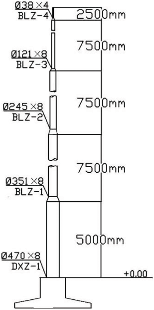
Figure 1: Structure diagram of the independent lightning rod
In order to simulate the three-dimensional flow around the lightning rod in a wind field, the computational grid for the entire structure can reach a scale of billions of grid cells when the grid resolution meets the accuracy requirements of the viscous sublayer calculation. This requires significant computational resources and time. Therefore, in this study, the three-dimensional flow around the lightning rod structure is approximated by simulating the flow around five cylinders with different diameters.
The computational domains corresponding to each segment of the lightning rod are shown in Fig. 2. D represents the diameter of the corresponding segment. The distance from the center of the cylinder to the upper and lower boundaries is set to 7D. The distance from the center of the cylinder to the inlet boundary is set to 10D, while the distance to the outlet boundary is set to 25D. The length of the cylinder, which corresponds to the thickness of the computational domain, is set to D. Similar boundary conditions are applied to the computational domains of different segments: the inlet boundary is set as a velocity inlet, the outlet boundary is set as an outflow, and the cylinder walls are set as no-slip walls. The remaining boundaries are set as symmetries.
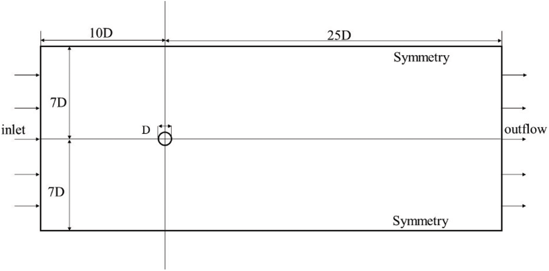
Figure 2: Schematic diagram of the flow field computational domain
Based on the terrain roughness of the area where the 330 kV lightning rod is located, it can be determined that it belongs to the Class B terrain according to the “Load code for the design of building structures” (GB 50009-2012) in China. According to the expression (1) for the power law wind speed profile in the “Load code for the design of building structures” (GB 50009-2012) [15], the corresponding wind speed at a given height can be calculated as follows:
where α is taken as 0.15 for Class B terrain.
To simulate and analyze the flow field for different segments at the same reference wind speed and for the same segment at different reference wind speeds, the following parameters were set, as shown in Table 1.

The surrounding region of the circular tube and the wake region are the key areas of concern for the flow simulation around the lightning rod. The grid division in the near-wall region of the circular tube significantly affects the accuracy of the calculation results. Therefore, appropriate grid division is required for these areas. In this study, the Y+ value is used to control the boundary layer grid division.
The Y+ value is a dimensionless number that measures the height of the first layer. For the SST k-ω model, it is recommended that the Y+ value should not exceed 1.0. Therefore, in this study, the Y+ value is set to 1.0 for subsequent calculations to ensure accuracy.
The process of calculating the height of the first layer based on the Y+ value is as follows [16]:
1. Calculate the Reynolds number:
2. Calculate the wall friction coefficient:
3. Calculate the wall shear stress:
4. Calculate the friction velocity:
5. Calculate the height of the first grid layer:
Where ρ represents the fluid density (with a value of 1.225 kg/m3), v is the incoming velocity, l is the characteristic dimension, and μ is the dynamic viscosity coefficient (with a value of 1.79 × 10⁻⁵ Pa).
Considering the distribution characteristics of the flow field and the required computational accuracy [17], the flow field region around the lightning rod is divided into surrounding region, near-wall region, and wake region. A hexahedral-dominant method is employed for grid generation. The grid is locally refined in the critical areas around the circular tube and in the wake region. In the near-wall region of the circular tube, boundary layer grids are generated, with the height of the first layer determined by the previous calculation using the Y+ value.
2.3 Turbulence Model and Simulation Setup
Roughly speaking, turbulence is generated due to the instability of the system during fluid flow. Generally, in two-equation models, the k-epsilon (k-ε) model is suitable for simulating fully-developed turbulence away from the wall, while the k-omega (k-ω) model provides good accuracy and stability for simulation in the near-wall region. The SST k-ω turbulence model used in this study combines the advantages of these two models. By using a blending function, the k-ω model is employed near the wall, while the k-ε model is used in free shear layer and the region away from the wall. The SST k-ω model exhibits good computational performance and has been widely applied in engineering [18,19].
According to the “Load code for the design of building structures” (GB 50009-2012), an empirical formula is provided for the along-wind turbulence intensity [15]:
For different types of terrains (A, B, C, D), the values of I10 are 0.12, 0.14, 0.23, and 0.29, respectively. By using Eq. (2), the turbulence intensity at the midpoint of each segment of the lightning rod in B-class terrain can be calculated, as shown in Table 2.

In this paper, the SIMPLE algorithm is initially used for steady-state calculations. The initial iteration steps are set to 300, which may vary depending on the convergence. Once the flow has sufficiently developed, the PISO algorithm is used for transient calculations to obtain the temporal variations of the physical quantities. The convergence criteria are set as follows: continuity residual of 10−4, velocity residual of 10−6, turbulent kinetic energy residual of 10−5, and turbulent dissipation rate residual of 10−5.
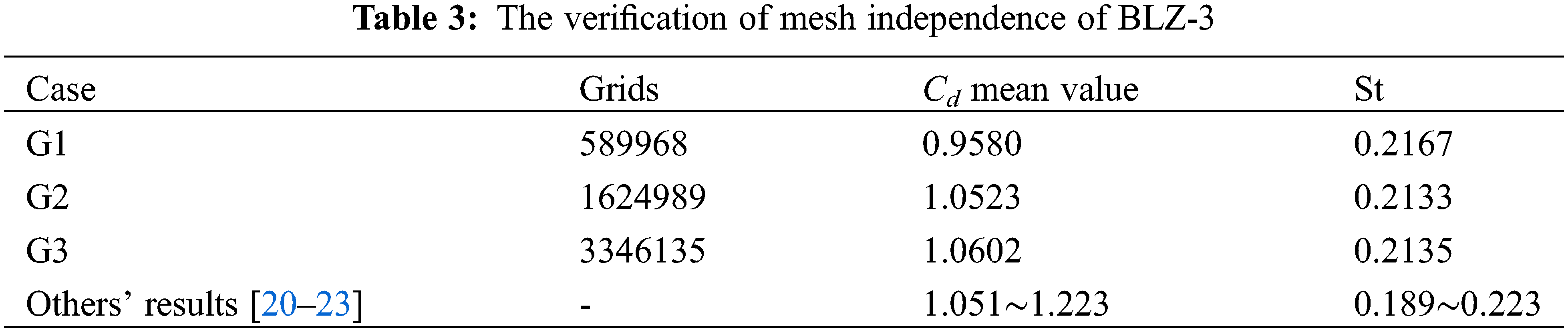
2.4 The Verification of Mesh Independence
The verification of mesh independence of BLZ-3 is taken as an example here. As shown in Table 3, three sets of mesh were employed to the simulation of BLZ-3 under the same parameters. The mean value of drag coefficient Cd and Strouhal number St were obtained and compared with experiment and simulation results of others. It can be observed that the numerical simulation results of case G2 and G3 are in good agreement with others’ results, and the differences between the calculated results of G2 and G3 are relatively small. Therefore, it can be considered that the grid accuracy of G2 meets the computational requirements. Consequently, G2 is adopted as the final grid for the BLZ-3 segment.
3.1 Vortex Shedding Phenomenon
Figs. 3a–3e illustrate the vortex contour maps for the BLZ-4, BLZ-3, BLZ-2, BLZ-1, and DXZ-1 sections at a reference wind speed of 5 m/s, which are obtained using the Q-criterion.
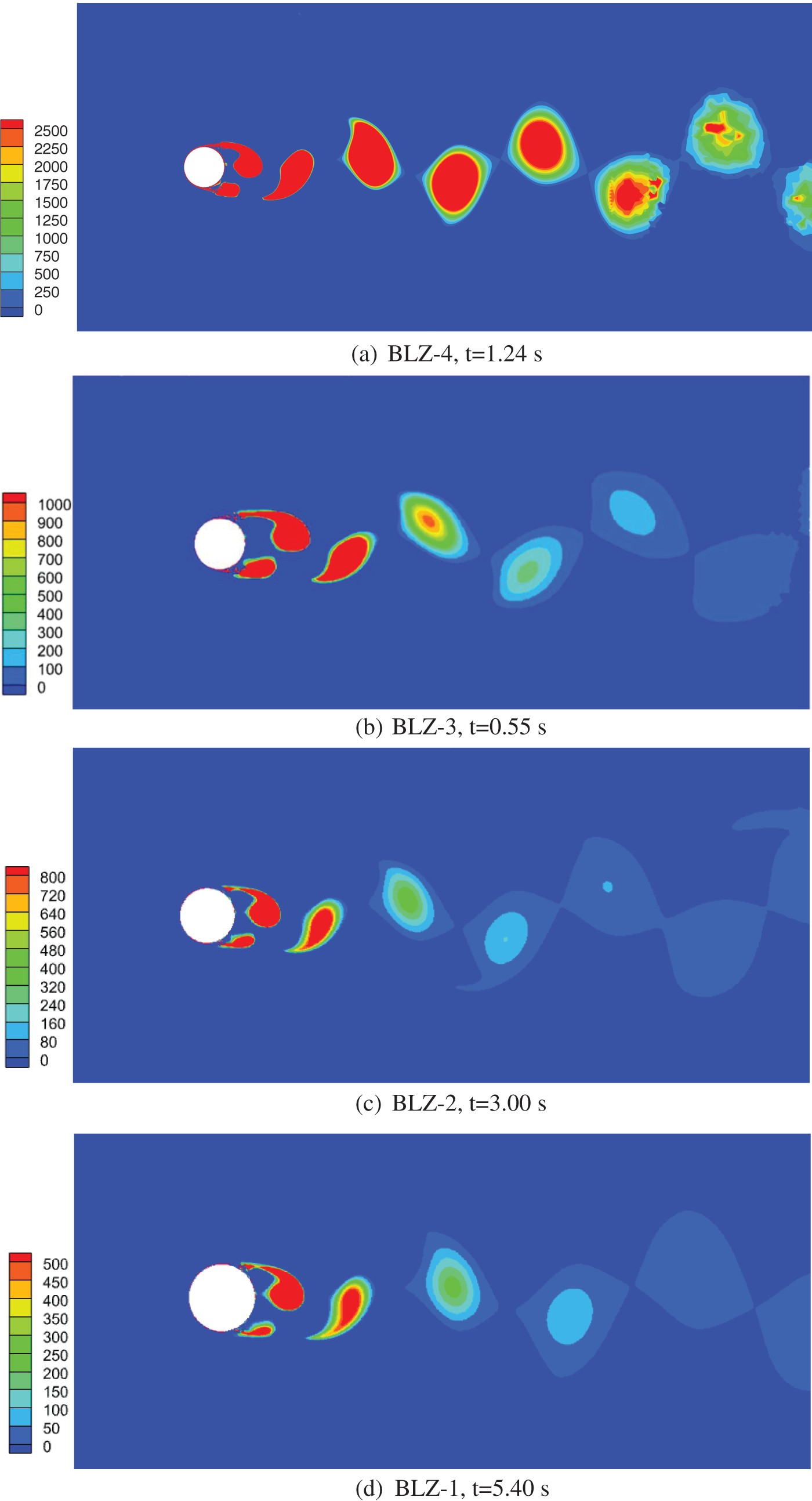
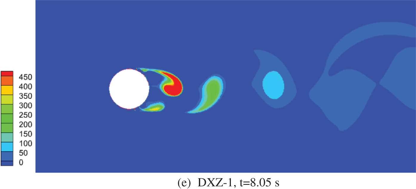
Figure 3: Vortex contour maps of lightning rod sections
It can be concluded from figures above that:
(1) In Fig. 3, a regular pattern of alternating and staggered vortical structures can be observed in the wake region behind the cylinder. This indicates the formation of organized vortex shedding.
(2) The vortices in the wake region exhibit a gradual increase in size and a decrease in vorticity magnitude. This suggests that energy dissipation occurs as the vortices move downstream.
(3) Comparing these five figures, it can be observed that as the diameter of the cylinder decreases, the magnitude of vorticity increases, indicating a stronger vortex shedding phenomenon.
Additionally, Figs. 4a–4e provide velocity vector maps at corresponding time frames for the sections of the lightning rod, allowing for a comparative analysis of the flow patterns.
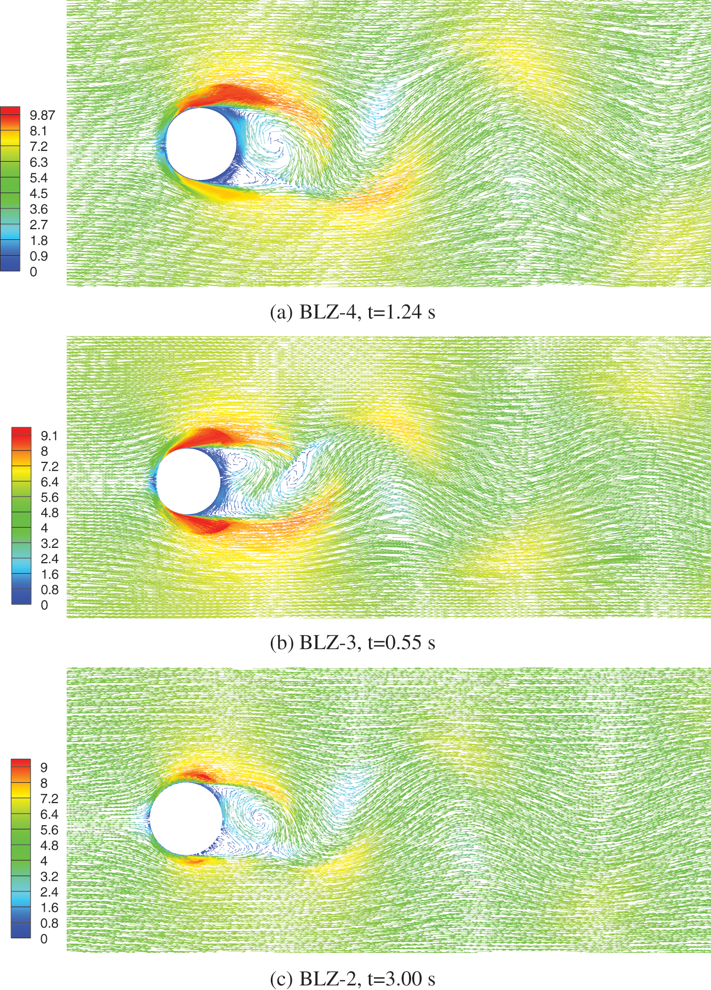
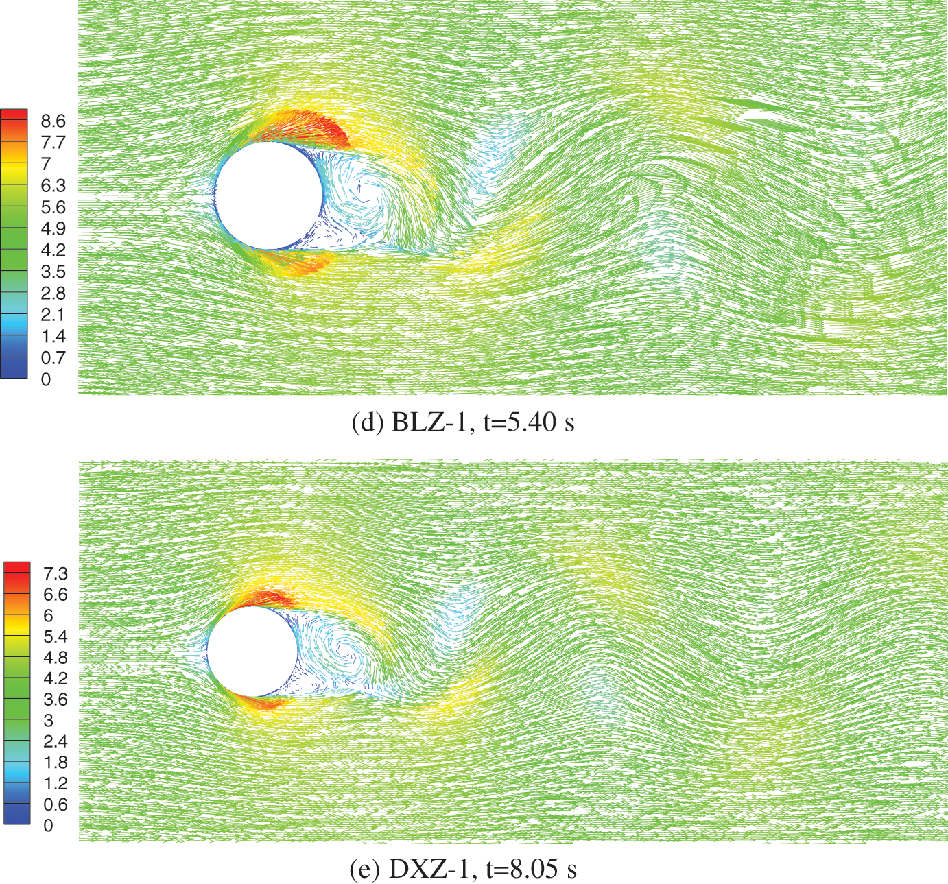
Figure 4: Speed vector maps of lightning rod sections
The following observations can be made from Fig. 4:
(1) After the airflow reaches the surface of the cylinder, the airflow velocity at the top of the windward surface becomes zero. This point is called the stagnation point. Subsequently, the airflow splits into two streams along the upper and lower surfaces of the cylinder.
(2) As the airflow passes along the windward half of the cylinder’s surface, the velocity increases continuously and exceeds the incoming wind speed. On the leeward half of the cylinder’s surface, the velocity decreases continuously, and a reverse flow region can be observed.
(3) On the leeward side of the lightning rod, vortices are formed due to the airflow, and with the progression of time, the shedding of vortices occurs.
3.2 Lift and Drag Coefficient Analysis
The lift coefficient Cl and drag coefficient Cd are important parameters that characterize the effect of flow on a cylinder. They are defined as follows:
Under the condition of a reference wind speed of 5 m/s, the flow analysis is conducted for each segment of the lightning rod. This allows us to obtain the time history curves of the drag coefficient and the lift coefficient (Figs. 5a–5e) for each segment. The drag coefficient is calculated according to Eq. (3), while the lift coefficient is calculated according to Eq. (4).
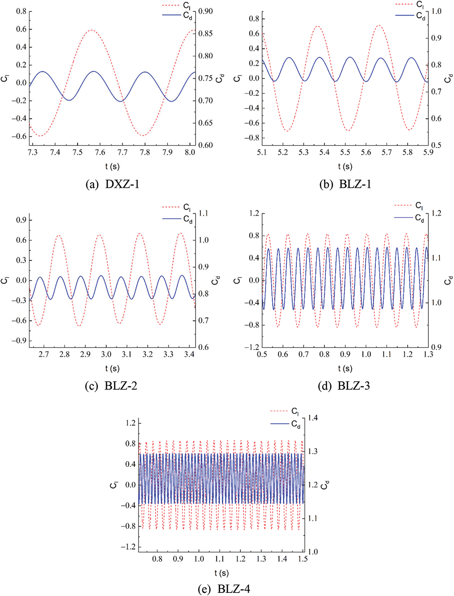
Figure 5: Time history curve of lift and drag coefficients for different segments
From Figs. 5a–5e, it can be observed that both the drag coefficient and the lift coefficient exhibit stable sinusoidal waveforms over time. Additionally, the lift and drag coefficient curves for different diameter cylinders show different frequencies.
By analyzing the time history curves of the drag coefficient and lift coefficient for each segment of the lightning rod after reaching a stable state, we can obtain their mean values and RMS magnitudes. Furthermore, by performing a fast Fourier transform on the time history curves of the drag coefficient and lift coefficient, we can obtain the frequencies of the lift and drag coefficients for each segment, as shown in Table 4.

From Table 4, it can be observed that from DXZ-1, BLZ-1, BLZ-2, BLZ-3 to BLZ-4, the mean value, RMS magnitude, and frequency of the drag coefficient, as well as the RMS magnitude and frequency of the lift coefficient, increase with the decrease in diameter of the lightning rod segments. Furthermore, the frequencies of the drag coefficients for different segments are approximately twice the frequencies of the lift coefficients.
Based on the numerical analysis of the lift and drag coefficients for different segments of the lightning rod at the same reference wind speed, further analysis is conducted on the variation characteristics of the lift and drag coefficients for the same lightning rod segment at different reference wind speeds. Figs. 6a–6d show the lift coefficient, drag coefficient curves, and their spectral analysis for the BLZ-3 segment at reference wind speeds of 5, 10, 15, and 20 m/s, respectively. Table 5 provides additional parameters of the flow around the segment under these conditions, including the Reynolds number, root mean square values of the lift and drag coefficients, and the vortex shedding frequency of the cylinder.
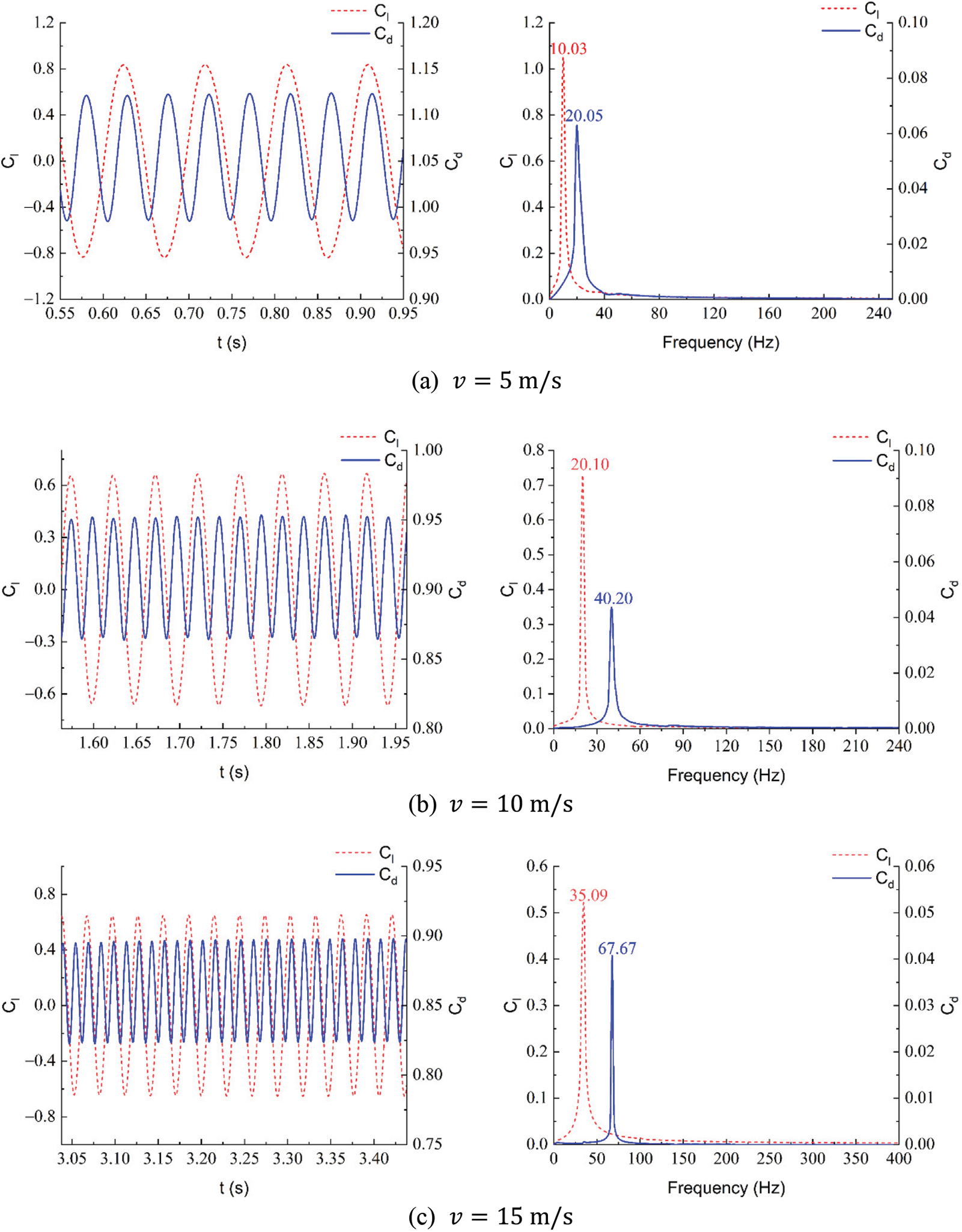
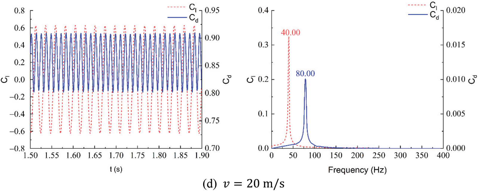
Figure 6: Time histories and frequency analysis of lift and drag coefficients at different wind speed

From the time-domain curves in Fig. 6, it can be observed that after reaching a stable state, the lift and drag coefficients on the surface of the cylinder exhibit oscillatory variations. This is due to the shedding of vortices, which leads to pressure fluctuations in the flow field and consequently causes the forces on the cylinder surface to oscillate. The lift coefficient fluctuates sinusoidally around zero, while the drag coefficient fluctuates sinusoidally around a value greater than zero.
Further analysis of the frequency characteristics of the lift and drag coefficients under different wind speeds reveals that the lift and drag coefficient curves approximate sinusoidal waves with complete periodicity. They exhibit a single dominant peak frequency, and the peak frequency of the drag coefficient is approximately twice that of the lift coefficient. According to Table 5, as the wind speed increases, the vortex shedding frequency, which is also the frequency of the drag coefficient, increases. Moreover, as the wind speed increases from 5 to 20 m/s, the root mean square values of the lift and drag coefficients decrease.
The same parameters of flow around other segments at different reference wind speeds were also investigated and listed below in Table 6, from which similar conclusions could be drawn.

3.3 The Relationship of Lift Coefficient, Drag Coefficient, and Vorticity Distribution
In this section, the time-history curves of lift and drag coefficients for the BLZ-3 segment at a reference wind speed of 5 m/s are presented in Fig. 7, along with the corresponding vorticity distribution at key time frames shown in Figs. 8a–8d, to illustrate their relationships.
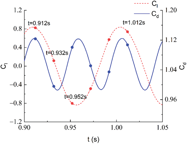
Figure 7: Lift coefficient and drag coefficient of BLZ-3
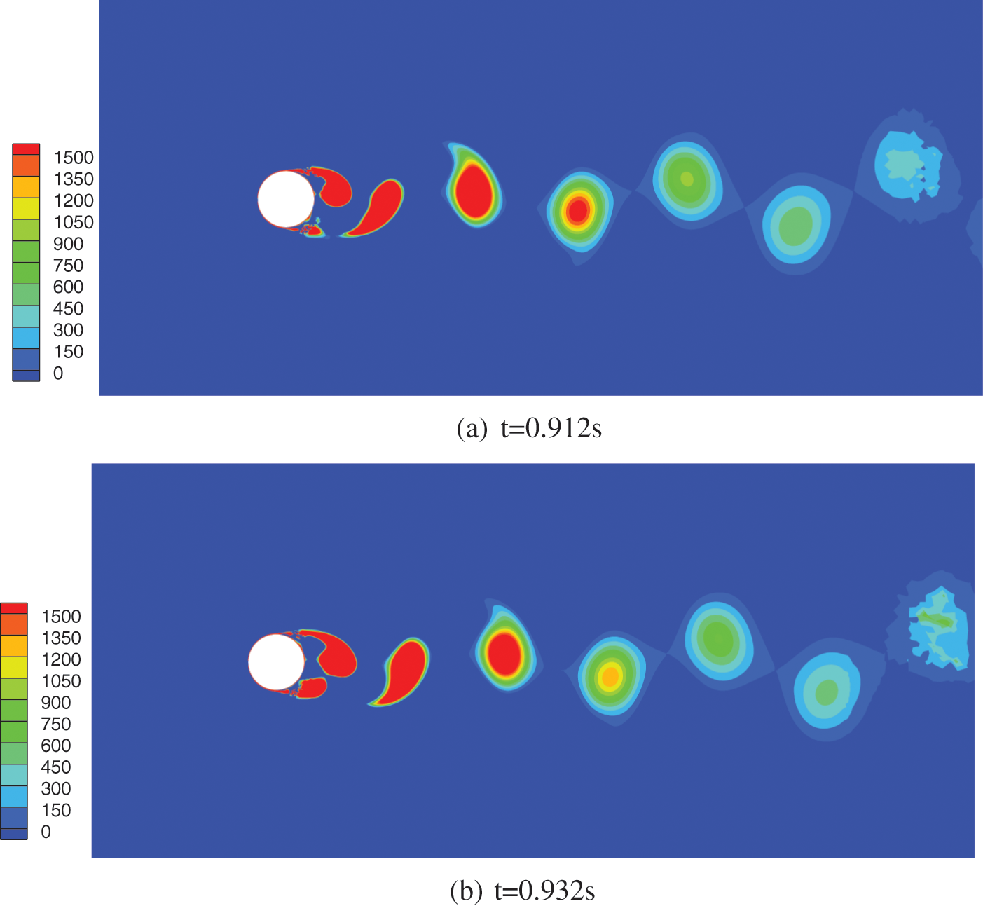
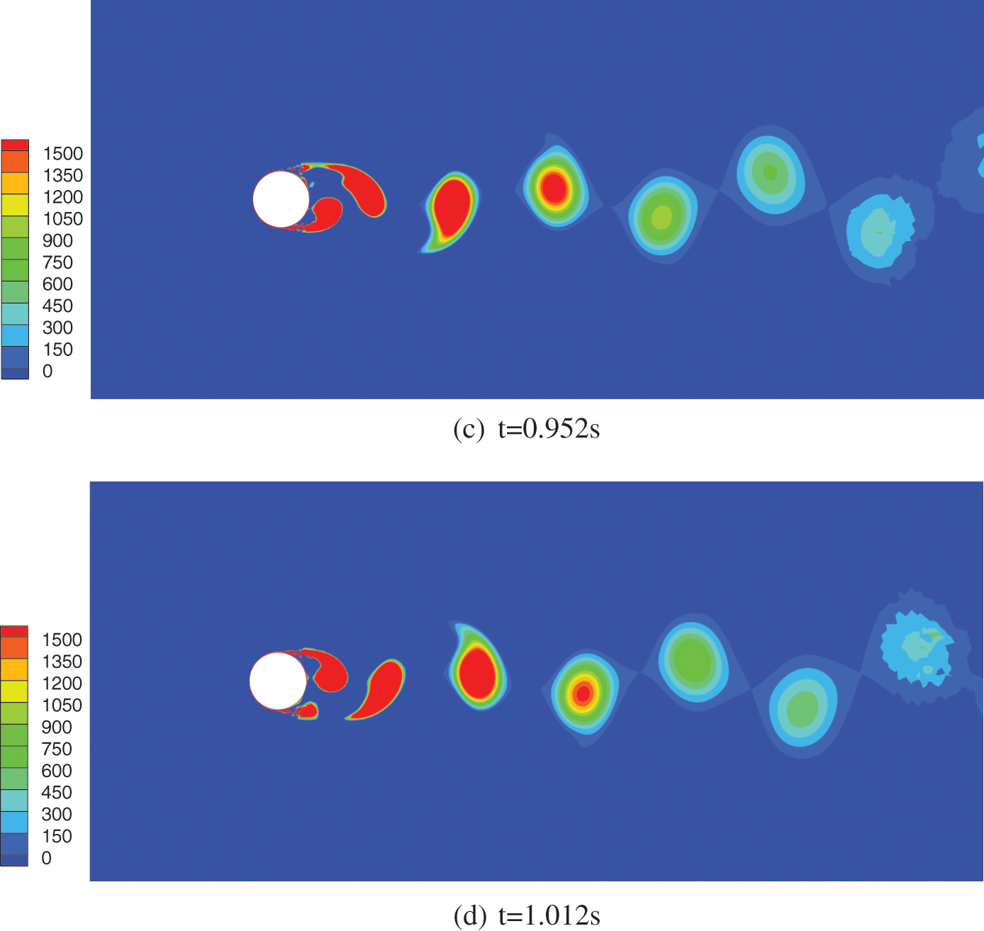
Figure 8: Vorticity distribution of BLZ-3 at corresponding timeframe
At t = 0.912 s, vortex shedding occurs on the lower side of the cylinder, resulting in both lift and drag coefficients reaching their peak values. Subsequently, both coefficients start to decrease. At t = 0.932 s, no vortex shedding is observed on the cylinder’s lateral surface, and the drag coefficient reaching its minimum value while the lift coefficient continues to decrease. At t = 0.952 s, vortex shedding occurs on the upper side of the cylinder, causing the drag coefficient to reach its peak value again, and the lift coefficient to reach its minimum value. Finally, at t = 1.012 s, vortex shedding occurs again on the lower side of the cylinder, and both lift and drag coefficients once again reach their peak values.
It can be observed that when vortex shedding occurs on the cylinder’s lateral surface, the drag coefficient reaches its peak value, while the corresponding lift coefficient alternates between peak and trough values. The time difference between two vortex shedding events on one side of the cylinder corresponds to one cycle of the lift coefficient.
In this paper, numerical simulations were conducted using the computational fluid dynamics method with ANSYS Fluent. The flow field around a 330 kV cylindrical lightning rod was simulated to investigate and compare the lift and drag coefficients of different sections of the lightning rod at the same reference wind speed of 5 m/s, and the variations of lift and drag coefficients for the same lightning rod section at different reference wind speeds were analyzed. The following main conclusions were drawn:
1. The presence of the cylindrical steel tube obstructs incoming flow, causing velocity redistribution in the flow field. This leads to higher velocities on the tube’s lateral sides and lower velocities on the windward and leeward surfaces, creating vortex shedding in the wake region.
2. All sections of the lightning rod demonstrate vortex shedding phenomena. The shedding of vortices results in the oscillation of lift and drag coefficients on the lightning rod surface. The time-domain curves of lift and drag coefficients exhibit sinusoidal patterns with a single peak frequency.
3. Segments with smaller diameters exhibit more pronounced vortex shedding, higher vortex intensities, and larger root mean square magnitudes of lift and drag coefficients at the same reference wind speed.
4. In a certain range, increasing wind speed leads to reduced root mean square values of lift and drag coefficients.
Acknowledgement: None.
Funding Statement: This study was supported by State Grid Ningxia Electric Power Co., Ltd. under Grant 5229CG220006 and Natural Science Foundation of Ningxia Province under Grant 2022AAC03629.
Author Contributions: The authors confirm contribution to the paper as follows: study conception and design: Wei G, Bo H; simulations: Jiazheng M, Mengqin H; analysis and interpretation of results: Yanliang L, Xuqiang W, Jiazheng M, Mengqin H; draft manuscript preparation: Jiazheng M, Mengqin H. All authors reviewed the results and approved the final version of the manuscript.
Availability of Data and Materials: The data that support the findings of this study are available from the corresponding author, upon reasonable request.
Conflicts of Interest: The authors declare that they have no conflicts of interest to report regarding the present study.
References
1. Zhao, G., Li, J., Zhang, M., Yi, Y. (2022). Experimental study on the bearing capacity and fatigue life of lightning rod structure joints in high-voltage substation structures. Thin-Walled Structures, 175, 109282. [Google Scholar]
2. Huang, Z., Shu, Y. (2019). Research on P-Δ effect increase coefficient of independent steel tube lightning rods in substation. IOP Conference Series: Earth and Environmental Science, 310(3), 032073. [Google Scholar]
3. Chen, G., Chen, Y., Chen, Y., Ji, S. (2020). Dynamics modeling and experimental modal analysis of bolt loosening for lightning rod. Journal of Vibroengineering, 22(3), 657–671. [Google Scholar]
4. Zandbergen, P. J., Dijkstra, D. (1987). Von Kármán swirling flows. Annual Review of Fluid Mechanics, 19(1), 465–491. [Google Scholar]
5. O’Malley, R. E. (2014). Ludwig prandtl’s boundary layer theory. In: Historical developments in singular perturbations. Switzerland: Springer, Cham. [Google Scholar]
6. Bouard, R., Coutanceau, M. (2006). The early stage of development of the wake behind an impulsively started cylinder for 40 < Re < 104. Journal of Fluid Mechanics, 101(3), 583–607. [Google Scholar]
7. Travin, A., Shur, M., Strelets, M., Spalart, P. (2000). Detached-eddy simulations past a circular cylinder. Flow, Turbulence and Combustion, 63(1), 293–313. [Google Scholar]
8. Mathupriya, P., Chan, L., Hasini, H., Ooi, H. (2018). Numerical study of flow characteristics around confined cylinder using OpenFOAM. International Journal of Engineering & Technology, 7(4), 617–623. [Google Scholar]
9. Chadwick, E., Christian, J., Chalasani, K. (2018). Using eulerlets to model steady uniform flow past a circular cylinder. European Journal of Computational Mechanics, 27(5–6), 469–478. [Google Scholar]
10. Loc, T., Bouard, R. (1985). Numerical solution of the early stage of the unsteady viscous flow around a circular cylinder: A comparison with experimental visualization and measurements. Journal of Fluid Mechanics, 160, 93–117. [Google Scholar]
11. Kusyumov, A. N., Kusyumov, S. A., Mikhailov, S. A., Romanova, E. V. (2021). Numerical simulation of 3D flow over a circular cylinder. Journal of Physics: Conference Series, 2057(1), 012072. [Google Scholar]
12. Nguyen, V. L., Degawa, T., Uchiyama, T., Takamure, K. (2019). Numerical simulation of bubbly flow around a cylinder by semi-Lagrangian–Lagrangian method. International Journal of Numerical Methods for Heat & Fluid Flow, 29(12), 4660–4683. [Google Scholar]
13. Kumar, V., Singh, M., Thangadurai, M., Chatterjee, P. K. (2019). Effect of free stream turbulence on flow past a circular cylinder at low reynolds numbers. Journal of the Institution of Engineers (IndiaSeries C, 100(1), 43–58. [Google Scholar]
14. Yuce, M. I., Kareem, D. A. (2016). A numerical analysis of fluid flow around circular and square cylinders. Journal AWWA, 108(10), E546–E554. [Google Scholar]
15. Ministry of Housing and Urban-Rural Development (2012). Load code for the design of building structures: GB 50009-2012. China: China Architecture & Building Press (In Chinese). [Google Scholar]
16. Zhou, J. Z., Xu, X. P., Chu, W. J., Zhu, Z. C., Chen, Y. H. et al. (2013). Analysis and simulation of the fluid field in thermal water-jet nozzle based on ANSYS FLUENT & ICEM CFD. Applied Mechanics and Materials, 423–426, 1677–1684. [Google Scholar]
17. Stringer, R. M., Zang, J., Hillis, A. J. (2014). Unsteady RANS computations of flow around a circular cylinder for a wide range of Reynolds numbers. Ocean Engineering, 87, 1–9. [Google Scholar]
18. Fan, J., Zhang, X., Cheng, L., Cen, K. (1997). Numerical simulation and experimental study of two-phase flow in a vertical pipe. Aerosol Science and Technology, 27(3), 281–292. [Google Scholar]
19. Tian, Y., Gao, Z., Jiang, C., Lee, C. H. (2022). A correction for Reynolds-averaged-Navier-Stokes turbulence model under the effect of shock waves in hypersonic flows. International Journal for Numerical Methods in Fluids, 95(2), 313–333. [Google Scholar]
20. Schewe, G. (1983). On the force fluctuations acting on a circular cylinder in crossflow from subcritical up to transcritical Reynolds numbers. Journal of Fluid Mechanics, 133, 265–285. [Google Scholar]
21. Norberg, C. (2003). Fluctuating lift on a circular cylinder: Review and new measurements. Journal of Fluid Mechanics, 17(1), 57–96. [Google Scholar]
22. Achenbach, E. (1971). Influence of surface roughness on the cross-flow around a circular cylinder. Journal of Fluid Mechanics, 46(2), 321–335. [Google Scholar]
23. Li, C. Z., Zhang, X. S., Hu, X. F., Li, W., You, Y. X. (2018). Study on multi-column flow characteristics under high Reynolds number. Chinese Journal of Theoretical and Applied Mechanics, 50(2), 233–243 (In Chinese). [Google Scholar]
Cite This Article
 Copyright © 2024 The Author(s). Published by Tech Science Press.
This work is licensed under a Creative Commons Attribution 4.0 International License , which permits unrestricted use, distribution, and reproduction in any medium, provided the original work is properly cited.
 Downloads
 Citation Tools