Research on Narrowband Line Spectrum Noise Control Method Based on Nearest Neighbor Filter and BP Neural Network Feedback Mechanism

1  Introduction

There are two different noise control strategies for noise pollution: passive control and active control. Passive noise control, also known as passive noise control, refers to the use of insulation, muffling, sound insulation and other passive methods to attenuate noise [1]. Active noise control (ANC), also known as active noise control is a noise elimination technology based on the principle of acoustic superposition phase elimination. It works on the principle that the ANC system generates an anti-noise with equal amplitude and opposite phase to the main noise, which is superimposed and canceled at the error microphone to achieve the noise reduction effect [2].

Generally speaking, ANC is used to adjust the control weights of the adaptive filter by minimizing the error signal. FxLMS is the most well-known adaptive filtering algorithm in the field of ANC. The algorithm works by first estimating the secondary path from the secondary source to the error microphone, and then using the estimated secondary path to filter the reference signal as the input to the controller, effectively reducing the effect of the secondary channel [3]. FxLMS has the advantages of small computation, easy implementation, and robustness, but the traditional fixed-step FxLMS suffers from the shortcomings of mutual constraints of convergence speed and steady-state error [4]. Therefore, many new adaptive algorithms are proposed in order to make up for the shortcomings of traditional adaptive filtering algorithms, improve the control performance of ANC systems, and meet diversified control requirements. Among them, the improvement of the traditional FxLMS and the application of deep learning are two hot spots.

The research of adaptive filtering algorithm and the application of neural network are the hot research topics in the field of active noise control in recent years [5]. In order to reduce the performance limitations of traditional adaptive filtering algorithms such as FxLMS and meet the needs of different scenarios, many improved adaptive filtering algorithms, especially deep learning-based active control algorithms, have been proposed and applied, aiming to improve the performance of various aspects such as noise reduction, convergence speed and stability, and have achieved good control results [6]. Zhang et al. proposed an FxLMS algorithm that can automatically adjust the step size according to the error signal. The FxLMS algorithm can automatically adjust the step size according to the error signal to improve the convergence speed and noise reduction effect of the adaptive filtering method in HVAC systems. The convergence speed and noise reduction effect of the algorithm are demonstrated to improve the noise reduction effect by 19%, the mean square error (MSE) was reduced by 23%, and the convergence speed was improved by 29% [7]. Tian et al. studied and proposed a method to improve the ANC system performance method. By using the optimal step size in the FxLMS algorithm and implementing a delayed FxLMS algorithm in each adaptive trap, the system is able to better remove multiple frequencies from the noise and improve the efficiency and the noise reduction system [8]. Saravanan et al. proposed and developed a soft threshold based FxLMS (STFxLMS) algorithm with harmonic mean based variable step size (HMVSS). By continuously changing the step size of this algorithm corresponding to the input noise signal and the error signal recorded by the error microphone, the convergence rate of the ANC system to the desired output is improved. The improvement in noise reduction using HMVSS compared to fixed step size is demonstrated by computer simulations [9]. Chen et al. proposed a new algorithm called PFxLMS for active noise reduction. This algorithm uses variable step size based on noise signal prediction to achieve fast convergence while improving convergence accuracy. Simulation results show that the PFxLMS algorithm outperforms both the traditional FxLMS algorithm and the variable step FxLMS algorithm based on the inverse tangent function in terms of convergence speed and accuracy [10]. Song et al. proposed two new algorithms for active noise reduction control systems, namely, FxLMS/F and C-FxLMS/F. Among them, the FxLMS/F algorithm is a variable-step version of the commonly used FxLMS algorithm, which aims to improve the noise reduction performance and convergence speed. The C-FxLMS/F algorithm is a combination of FxLMS/F and FxLMS algorithms, which can further improve the algorithm performance. It is demonstrated by simulation that the proposed algorithm outperforms the FxLMS algorithm under various noise input conditions, and the computational complexity and stability conditions are analyzed [11]. The multi-channel delayed adaptive trapping proposed by Zhang et al. can be directly applied to the active control of vehicle engine noise and other similar narrowband noise reduction. The algorithm can effectively reduce the vehicle internal engine noise with prominent harmonic characteristics, achieve a noise reduction of 4.05 dB in the time domain, and is also effective under non-smooth operating conditions, while a new time lag method is proposed to simplify the filtering process of the reference signal and greatly improve the computational efficiency of the algorithm [12]. Li et al. designed a new algorithm called enhanced diffusion FxLMS, which is a distributed control strategy for multi-channel active noise control systems that can overcome the limitations of existing distributed active noise reduction systems [13]. Kalaivani et al. used simulation software to analyze the control performance of various real-time recorded noise signals using LMS, NLMS and FxLMS algorithms based on parameters such as RMSE, SNR and convergence time [14]. Cha et al. proposed a new method called DNoiseNet to design a deep learning-based feedback active noise controller that can effectively eliminate various types of higher-order nonlinear noise, addressing the limitations of traditional active noise control methods, and developed a multilayer perceptron (MLP) neural network based on the two-level path estimator to improve the performance of DNoiseNet [15]. Zhang et al. proposed a method to reduce the delay of the deep ANC algorithm, which is a system used for noise cancellation. The algorithm uses a thoughtful recurrent network with smaller frame sizes, delay-compensated training, and a modified OLA to achieve zero or even negative algorithmic latency [16]. Zhang et al. introduced a multi-channel active noise control (ANC) method based on deep learning. The method, called the deep MCAC method, uses a convolutional recurrent network (CRN) for complex spectral mapping, where the total power of the error signal is used as a loss function for CRN training. Robustness against various noises is achieved by large-scale training. The results show that deep MCNC is effective for broadband noise reduction and has good generalization to untrained noise [17]. Im et al. proposed a deep learning-assisted secondary path update technique where neural networks are trained to estimate secondary paths in real time based on changing boundary conditions and by moving error sensors in the pipeline to simulate changes in boundary conditions, and it was demonstrated that ANC systems equipped with the update scheme were able to reduce broadband noise by up to 10 dB [18]. A deep learning based secondary path decoupled ANC (SPD-ANC) algorithm was proposed by Chen et al. A secondary path decoupling module consisting of two time-domain convolutional recurrent networks is used. Simulation results show that the algorithm outperforms traditional active noise reduction methods [19]. Jiang et al. used the nonlinear processing capability of neural networks to solve the nonlinear ANC problem, and the main idea is to use deep learning to encode the optimal control parameters for different noise environments. Firstly, the noisy signal is actively removed by the traditional adaptive filtering method, and then the residual noise and estimated noise are sent to the neural network to eliminate the nonlinear distortion. The experimental results show that the ANC system can be implemented by training the neural network with better noise reduction effect for both noisy and noisy speech [20]. Luo et al. proposed a simple and effective implementation of McFxLMS and McFxNLMS. Inspired by the backpropagation process during the training of neural networks, the McFxLMS and McFxNLMS algorithms can be implemented by an automatic derivation mechanism [21].

In this paper, considering the tracking performance and noise reduction performance when the noise signal is non-stationary, a new active control algorithm NNR-BPFxLMS based on nearest neighbor filter and neural network feedback mechanism is proposed. Simulations and experiments demonstrate that its stability, noise reduction, convergence speed and tracking performance are better than the traditional active control algorithm.

2  Feedback ANC System Based on NNR

2.1 ANC Systems and BP Neural Networks

The structure of the feedback ANC system is shown in Fig. 1a, where an NNR-based notch filter is used as the adaptive controller, whose detailed network structure is shown in Fig. 1b. An internal model estimation S^(z) is used to model the transfer function S(z) of secondary path. The input reference signal is obtained by adding error signal e(n) and S^(z) filtered-controller output y^s .

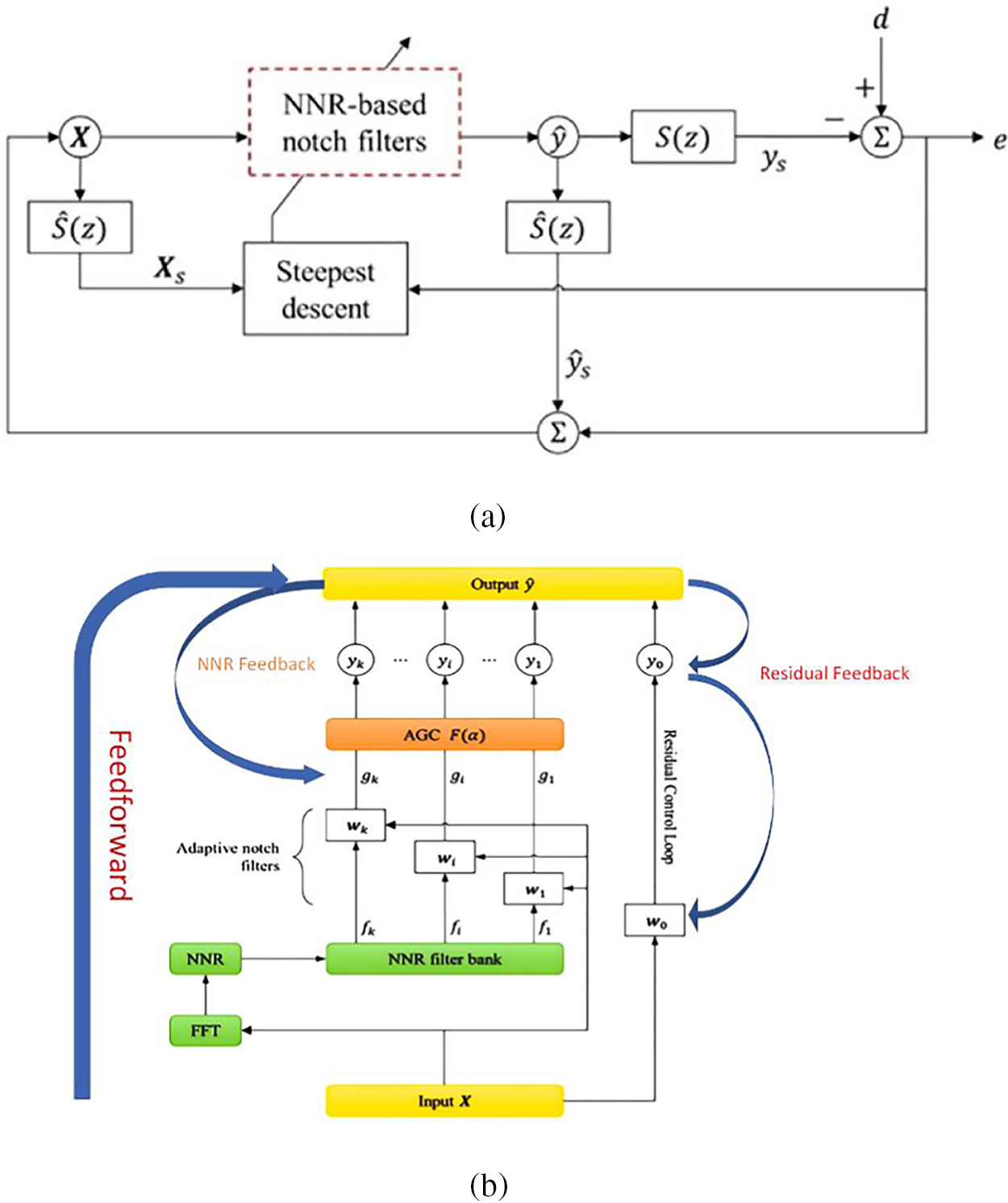
Figure 1: (a) Block diagram of the feedback ANC system and (b) control network structure based on NNR filter

The ANC controller consists of an adaptive notch filter and a residual control loop. In adaptive notch filters the line spectra f1, ⋯ , fk of the noise signal is firstly identified, which is used to calculate the corresponding filter coefficients w1,  ⋯ , w1 by the nearest neighbors regression. An adaptive gain controller (AGC) is used to tune the notch filters output g1,  ⋯ , gk. Additionally, input vector X is filtered by an LMS-based adaptive filter w0 for residual reduction.

2.2 Forward Propagation and Backward Propagation

In this paper, we implement the control network parameter update with the help of BP neural network for a given loss function. The basic BP algorithm consists of two processes: forward propagation of the signal and backward propagation of the error. That is, the error output is calculated in the direction from the input to the output, while the adjustment of the weights and thresholds is performed from the output to the input. In forward propagation, the input signal acts on the output node through the implied layer, and after the nonlinear transformation, the output signal is generated, and if the actual output does not match the desired output, it is transferred to the backward propagation process of the error. The error back-propagation is to back-propagate the output error through the hidden layer to the input layer by layer, and to apportion the error to all units in each layer, using the error signal obtained from each layer as the basis for adjusting the weights of each unit. By adjusting the connection strength of the input nodes to the hidden layer nodes and the connection strength of the hidden layer nodes to the output nodes as well as the threshold value, the error decreases along the gradient direction, and the training is stopped after repeated learning and training to determine the network parameters (weights and thresholds) corresponding to the minimum error.

3  Forward Propagation

3.1 Line Spectrum Identification Based on FFT

In this section, the noise signal sequence, which has been divided into several overlapping frames, is processed through FFT to obtain the instantaneous spectrum. The spectrum shown in Fig. 2a comes from the noise generated by a working motor, where line spectra are visible and broadband interference can be found in the frequency band above 500 Hz.

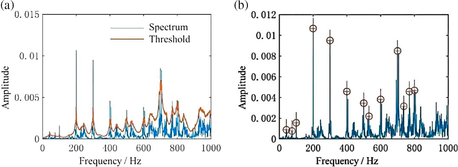
Figure 2: (a) Segmentation threshold and (b) identification results

Firstly, the forward moving average Af of the signal spectrum P1 is calculated, whose length is N, that is

 Af(1)=P1(1),  

Af(i)=ζAf(i−1)+(1−ζ)P1(i),  i=2, 3, ⋯, N,   (1)

where ζ=0.1 represents the average factor. Similarly, the back moving average Ab can be formulated as:

 Ab(N)=P1(N), 

Ab(i)=ζAb(i+1)+(1−ζ)P1(i),  i=N−1, N−2, ⋯, 1.  (2)

The segmentation threshold can be expressed by the sum of Af and Ab . Frequency whose amplitude exceeds the threshold is considered as line spectrum, so that

P2=max[0, P1−(Af+Ab)]. (3)

As shown in Fig. 2b, the adjacent line spectra are clustered to obtain the identification result.

3.2 Nearest Neighbor Regression and the Filter Bank

Most ANC systems based on FIR filters are applications of the Wiener filtering theory proposed in 1949. It is believed that the quadratic cost function of a stationary noise signal has a non-concave error surface, which means the control error can be minimized through an optimal filter.

Considering that the acoustic energy of discrete line spectral noise is mainly concentrated in the limited narrow bands, in this section a filter bank is established on the basis of the mapping relationship between the frequency of a pure tone signal and its optimal filter. The NNR is trained by the filter bank to calculate an approximate optimal filter a priori before controlling.

In this section, a set of optimal filters w1, w2, ···, wF of pure tones are calculated at 1 Hz intervals f = 1, 2, ···, F. Therefore, the NNR filters bank can be expressed as

Ω=[w1, w2, ⋯, wF]T.  (4)

The coefficients distribution of NNR filter banks is shown in Fig. 3, it can be found that the variation of the filter coefficients is continuous and periodic, which allows any filter unknown to be represented by the weighted sum of two neighboring filters in the database.

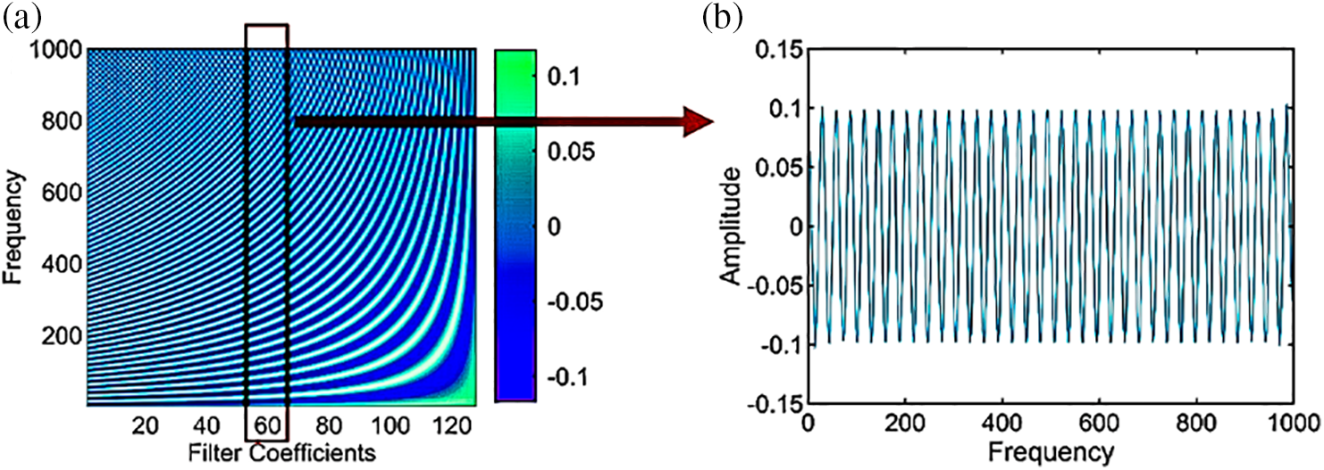
Figure 3: (a) The 2D heatmap of database and (b) distribution of one of the filter coefficients indicates that each parameter in database varies continuously

It should be noted that the filters bank shown in Fig. 3 represents only the case with specific parameters. The size of the filters bank is determined by the distribution of noise spectral lines. For example, it is necessary to increase the maximum frequency of the filters bank if high-frequency line spectral is found, which may consume more time to build the filters bank, but there is no additional computational cost in the control process.

The Nearest Neighbors Regression is a lazy learning method that uses interpolation to predict unknown filter coefficients with the ‘nearest’ samples in filters bank, whose training cost is zero.

For any line spectral frequency f that satisfies f∈(1, F) , there must exist natural numbers i and i+1 such that

i≤f≤i+1,  i=1, 2, ⋯, F−1.   (5)

Since the filter coefficients varies continuously with frequency, as shown in Fig. 4, linear interpolation is used to estimate wf , which is considered as the weighted sum of wi and wi+1 , that is

wf=ηwi+(1−η)wi+1,   (6)

where η=i+1−f.

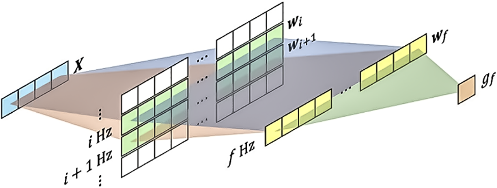
Figure 4: Calculate unknown filter coefficients using adjacent samples

So that the optimal notch filter wf corresponding to the unknown f can easily be estimated with wi and wi+1 , whose output gf can be expressed as

gf=X⋅wfT.  (7)

3.3 Adaptive Gain Controller

In this section, a nonlinear gain controller based on tanh function F(αf) is used to adjust the output of notch filters mentioned, that is

F(αf)=2⋅tanh⁡(0.55⋅αf),   (8)

where αi represents a linear gain factor. The function curve is as shown in Fig. 5, whose value range is (−2, 2) , and it has good linearity in the range of (−1, 1). As the gain F(αf) approaches the boundary, its rate of change will gradually decrease to 0.

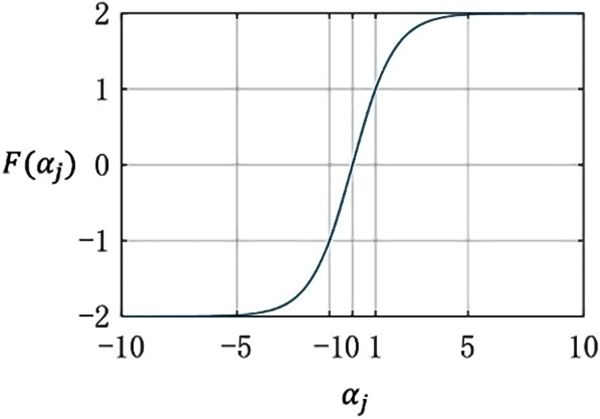
Figure 5: Function curve of the tanh-based nonlinear gain controller

Additionally, the derivative of the tanh function can be represented by itself, that is

F′(αf)=1.1⋅[1−tanh2(0.55⋅αf)]

=1.1⋅[1−F2(αf)4].  (9)

Therefore, the output of AGC can be formulated as

yf=F(αf)⋅gf.  (10)

3.4 The Residual Control Loop and System Output

The NNR-based notch filters have obvious control capability for line components within noise spectrum. In this section, an adaptive FIR filter w0 is used to reduce the residual broadband interference. The output of the residual control loop can be expressed as

y0=X⋅w0T.  (11)

For a noise signal consisting of k line spectra, the final output signal y^ is considered as the sum of a linear superposition of the NNR notch filters and the residual control loop, so that

y^=∑i=0k⁡yi

=y0+∑i=1k⁡F(αi)⋅gi  (12)

=Xw0T+∑i=1k⁡F(αi)⋅XwiT.

4  Backward Propagation

4.1 System Parameter Update

In this section, an internal model S^(z) is used to estimate the transfer function S(z) of the secondary path, whose impulse response can be expressed as h^s(n) and hs(n) . The computational graph is shown in Fig. 6.

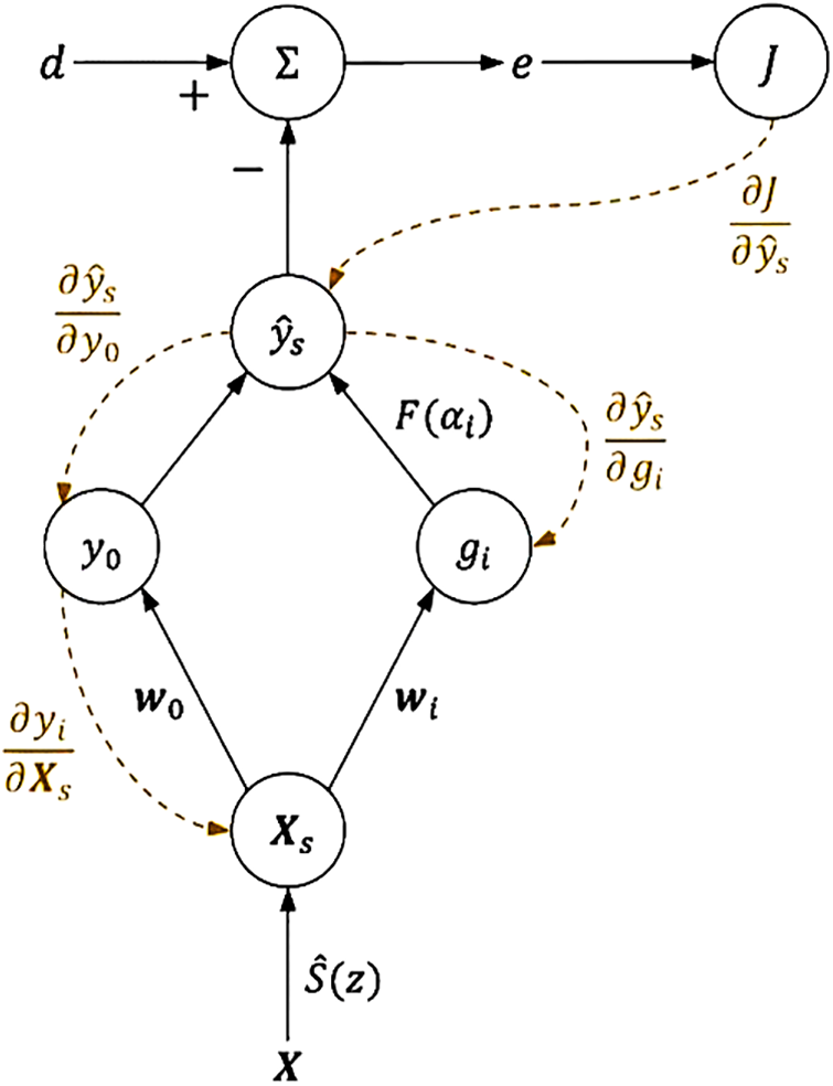
Figure 6: The computational graph of parameter update process

Instead of the input vector X, the filtered-X vector Xs(n)=X(n) ∗ h^s(n) is used as the bottom layer of computational graph, thus the gained notch filter output yi can be written as

yi=F(αi)⋅gi

=2tanh⁡(0.55αi)XswiT,  i=1, 2, ⋯, k.  (13)

Similarly, the residual control loop output can be expressed as

y0=Xsw0T.  (14)

Therefore, the filtered system output y^s can be formulated as

y^s=Xsw0T+∑i=1k⁡F(αi)⋅XswiT,  (15)

which should be equal to the actual secondary speaker output ys(n)=y^(n) ∗ hs(n) when S^(z)=S(z) the internal model can perfectly fit the secondary path. In this situation, error signal e(n) can be denoted by the filtered y^s , so that

e(n)=d(n)−y^s(n).  (16)

In this section, the mean square error (MSE) is used as the cost function J, that is

J=12[d(n)−y^s(n)]2.  (17)

The steepest descent algorithm is used to update the system parameters, thus the gradients Δαi and Δw0 is required, that is

Δαi=∂J∂αi,  i=1, 2, ⋯, k,  (18)

 Δw0=∂J∂w0. (19)

Expanded by the chain rule, Eq. (18) can be written as

∂J∂αi=∂J∂y^s∂y^s∂αi,   (20)

where:

∂J∂y^s=−[d(n)−y^s(n)]

=−e(n),   (21)

It can be known from Eq. (9) that

∂y^s∂αi=1.1⋅[1−F2(αi)4]gi

=1.1⋅[1−F2(αi)4]⋅XswiT,  (22)

Similarly, Eq. (19) can be expressed as

 Δαi=−1.1⋅[1−F2(αi)4]e(n)⋅XswiT,   i=1, 2, ⋯, k. (23)

Δw0=∂J∂y^s∂y^s∂w0=−e(n)Xs.  (24)

Moving the system parameters to the negative gradient direction by step μ , the new parameters can be formulated as

αi(n+1)=αi(n)+βe(n)⋅XswiT,  i=1, 2, ⋯, k

w0(n+1)=w0(n+1)+μe(n)Xs (25)

where:

β=μ[1−F2(αi)4].  (26)

5  Simulation and Experiments

5.1 Ideal Noise Control Experiments

In this section, an acoustic tube model shown in Fig. 7 was used to evaluate the performance of the proposed ANC system.

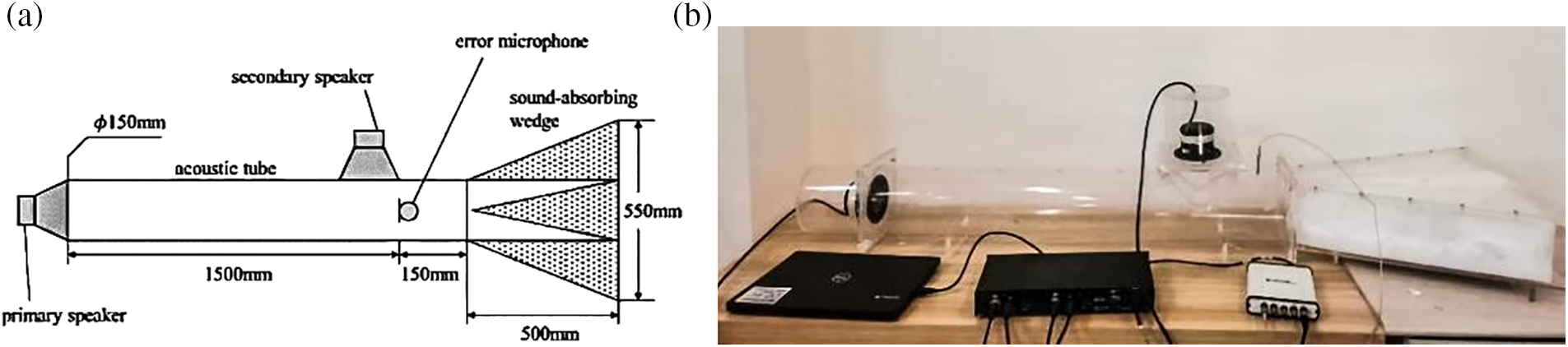
Figure 7: (a) Experimental schematic diagram and (b) physical diagram

As shown in Figs. 7a and 7b, a primary speaker was used to broadcast the noise signal and a secondary speaker was used to output the control signal. The error signal was obtained by an error microphone. The transfer function of secondary path was measured before experiment, whose frequency response is as shown in Fig. 8.

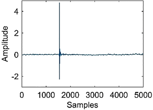
Figure 8: Impulse response of the secondary transfer function

The feedback FxLMS algorithm was selected as the baseline to compare with the NNR-based notch filters algorithm, and average noise reduction (ANR) was used as the evaluation criterion of the control algorithms.

ANR=20log⁡[Ae(n)Ad(n)]

Ae(n)=νAe(n−1)+(1−ν)|e(n)| (27)

Ad(n)=νAd(n−1)+(1−ν)|d(n)|, 

where Ae represents the average amplitudes of the error signal and Ad is the average amplitudes of desired noise signal with initial values Ae(0)=0 and Ad(0)=0 . The leakage factor was selected ν=0.995 .

In this section, a single-frequency noise signal was used to validate the NNR-based notch filters, whose spectrum was shown in Fig. 9. It can be found that there was a distinct line spectrum at 400.5 Hz with some harmonics and broadband interference.

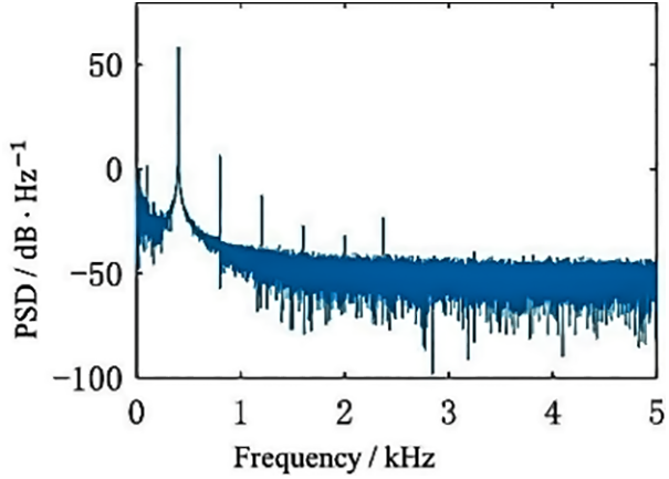
Figure 9: PSD of the noise signal

5.2 Convergence Speed and Stability Performance Analysis

The ANC systems had the same sampling rate Fs=2 kHz and FIR filter order L=128 , and the noise reduction curves of the chosen algorithms with different step size μ were shown in Fig. 10, whose convergence points have been marked by ‘⋆’ symbols.

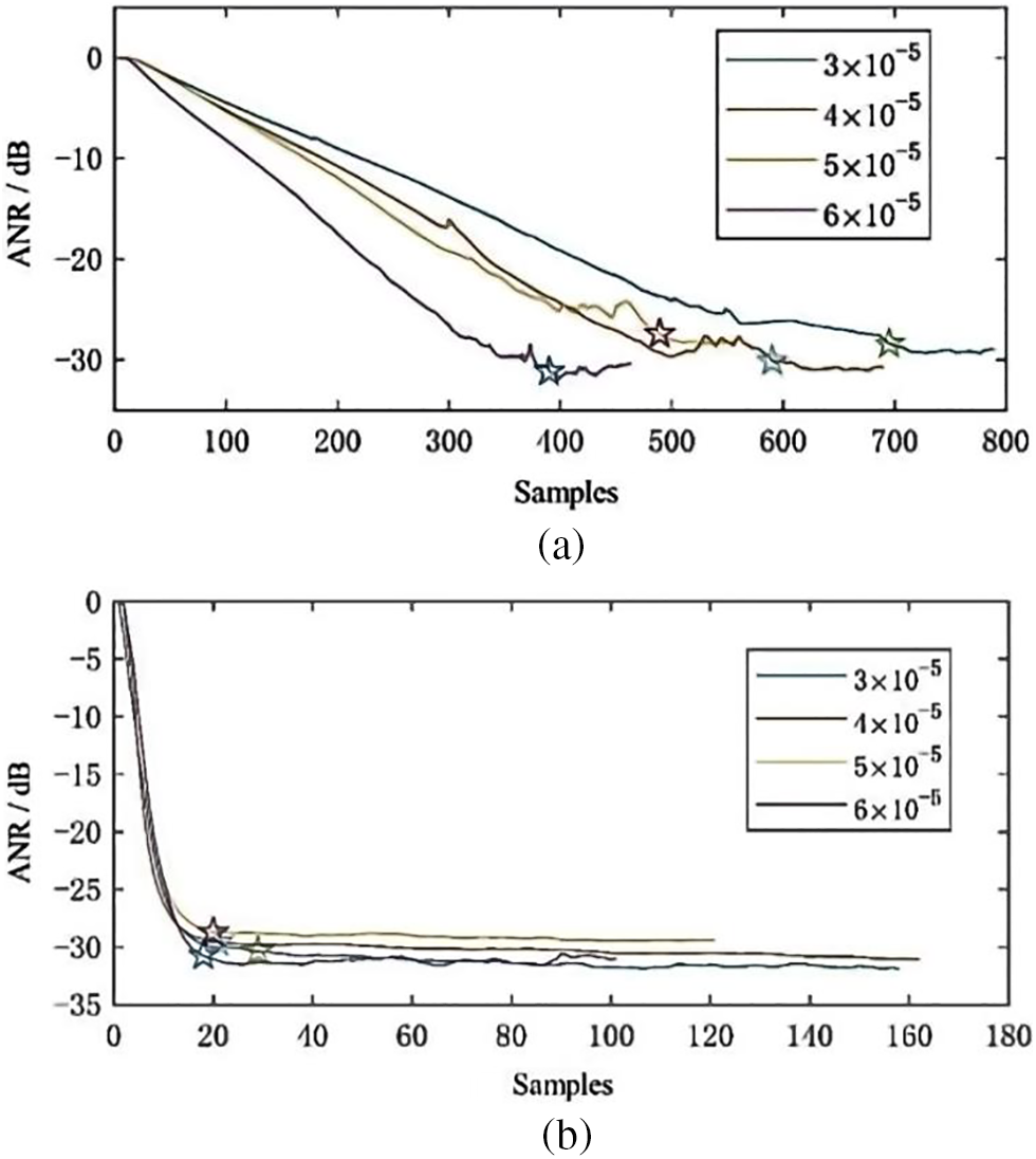
Figure 10: Noise reduction curve of (a) FxLMS and (b) NNR notch filter

As demonstrated in Fig. 10, the maximum ANR of FxLMS and NNR notch filters were similar. It can be found that FxLMS converged after at least 390 samples when μ=6×10−5 .

The convergence rate was accelerated linearly with the increase of step size μ . Otherwise, the reduction curves of NNR notch filters remained almost unchanged when step size varied. The convergence speed and steady-state error are not affected by the step size, overcoming the shortage of mutual constraints between the two traditional FxLMS algorithms, and the stability is effectively guaranteed. The convergence time of NNR notch filters was stable at about 25 samples, which was at least 95.38% faster than the FxLMS algorithm.

It can be concluded that under the same conditions, the performance of the NNR-BPFxLMS algorithm in this paper is not easily affected by the change of learning rate and possesses better stability and convergence speed, as shown in the following Table 1.

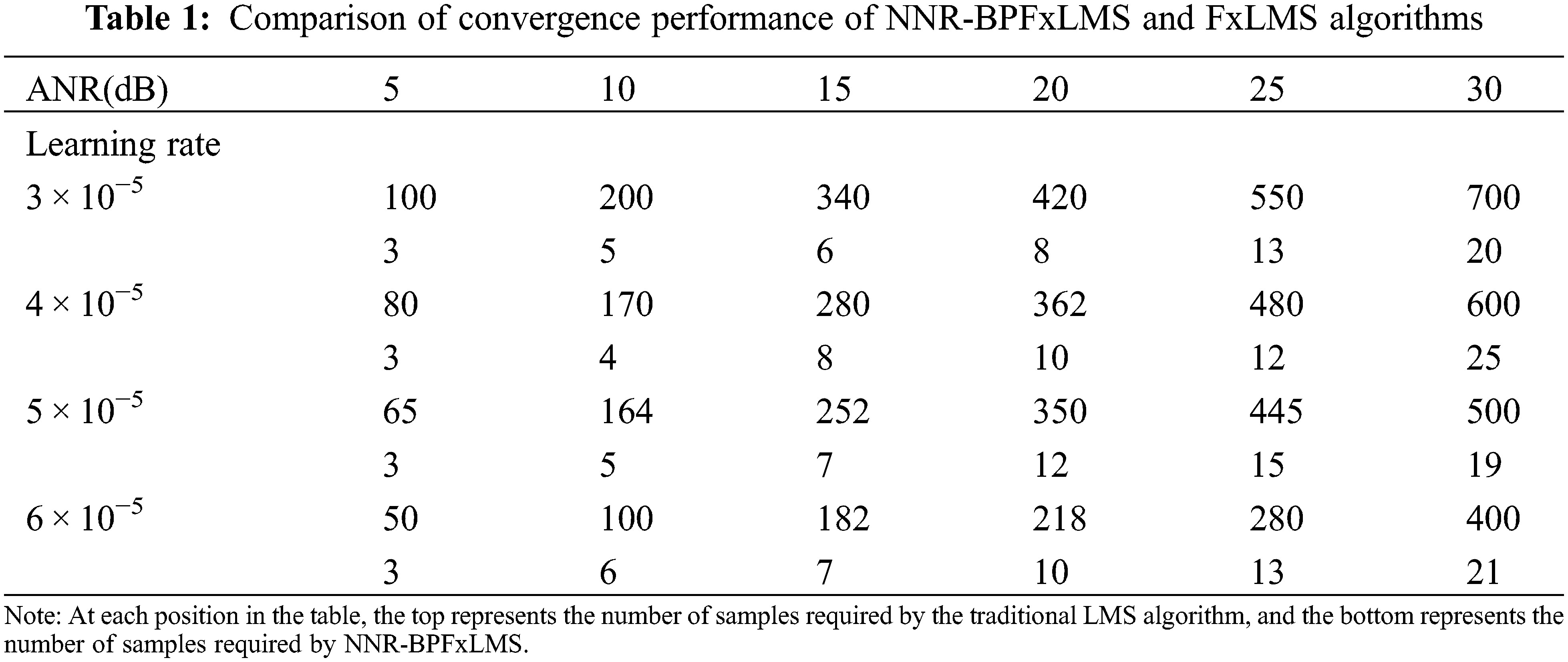
To sum up, the NNR-BPFxLMS requires only about 3% of the sampling points of the FxLMS to achieve the same amount of noise reduction with the same step size.

5.3 Complexity Analysis

The NNR-BPFxLMS algorithm uses the signal frequency as a feature to generate filter banks by interpolating adjacent training samples with 1 Hz interval. The approximate optimal filter coefficients are calculated beforehand, and the coefficients are further fine-tuned by a feedback control mechanism, and the computational effort for the fine-tuning part is small. Therefore, the main work in the system operation is to perform FFT on the signal, because there is a requirement for frequency resolution, so the number of FFT points will be relatively high, but this part of the system can be implemented asynchronously and will not affect the operation of the system.

5.4 Tracking Capability under Sudden Frequency Changes

Furthermore, another experiment was designed to verify the effectiveness of NNR notch filters where the noise signal spectrum had an abrupt change.

As demonstrated in Fig. 11, the noise signal consisted of two phases: there was a single 400.5 Hz line spectrum at the beginning, and another 700.2 Hz spectrum was added to form a dual-frequency signal after the controller converged. The step size was selected μ=5×10−5 and the reduction curves were shown in Fig. 12.

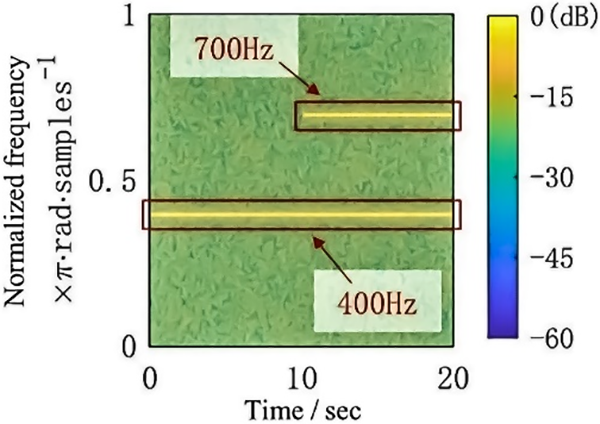
Figure 11: Spectrum of the noise signal with abrupt change

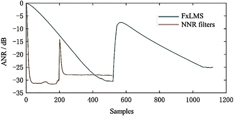
Figure 12: Convergence performance for the abrupt change signals

As demonstrated in Fig. 12, the convergence trend is basically consistent with that of Fig. 9, where FxLMS took 495 samples to restabilize after mutation, while the NNR-based algorithm took about 29 samples. It can be concluded that the NNR-BPFxLMS has faster tracking capability in the face of sudden changes in the frequency of noisy signals and can cope with the control requirements in complex noisy environments, which is of great significance for the research and control of non-smooth sudden change signals.

5.5 Computer Simulation Based on Real Noise

In this section, real noise data downloaded from Signal Processing Information Base (SPIB) was used to further research the feasibility and effectiveness of the NNR-based algorithm for actual control. The noise signal was acquired from a destroyer engine room, whose spectrum was shown in Fig. 13.

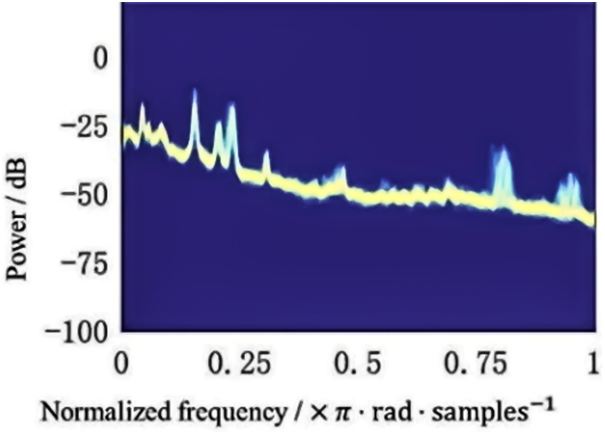
Figure 13: Spectrum of the destroyer engine room noise

As demonstrated in Fig. 13, the noise signal was normalized and consisted of several line spectra. The ANC systems had the same sampling rate Fs=19.98 kHz and FIR filter order L=128 . Assuming that S^(z)=S(z) , the noise reduction curves with different step size μ were shown in Fig. 14, where the control time of the simulation was 30 s.

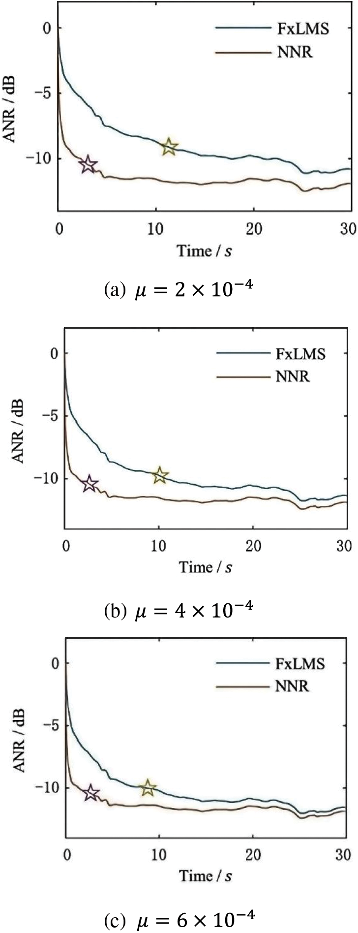
Figure 14: Convergence performance

To achieve a noise reduction of 5 dB, the FxLMS algorithm takes 2.13∼4.20 s, while NNR-BPFxLMS takes only 0.2 s or less to complete; to achieve a noise reduction of 5 dB, the FxLMS algorithm takes 9.37∼11.33 s, while NNR-BPFxLMS takes only about 3 s to complete. As demonstrated in Fig. 14, the convergence speed of FxLMS was accelerated as the step size increases. When the step size improved from 2×10−4 to 6×10−4 , the convergence time reduced from 11.33 to 9.37 s.

In contrast, the NNR-based notch filter was hardly affected by the change of step size and converged after about 2.64 s, which was optimized by 71.82% compared with the feedback FxLMS algorithm.

6  Conclusion

In this paper, for the line spectrum noise feedback control problem, the nearest neighbor regulator method is used for adaptive training of the trap filter, so that the ANC system learns an approximate optimal filter from the pre-trained NNR filter bank, and achieves system parameter changes with the help of the neural network feedback mechanism, thus shortening the convergence time.

It is demonstrated experimentally that the maximum noise reduction of the NNR-based trap filter is almost independent of the variation of system parameters such as step size and is almost the same as that of the conventional algorithm. Experimental and simulation results show that the convergence speed is accelerated by more than 95% when the signal spectrum is ideal, and increases by at least 71.82% for real noise.

Acknowledgement: The authors would like to thank the members of the School of Civil Engineering of Tianjin University.

Funding Statement: This work was supported by the National Key R&D Program of China (Grant No. 2020YFA040070).

Author Contributions: Study conception and design: Shuiping Zhang, Jun Tang; data collection: Xi Liang,Lei Yan; analysis and interpretation of results: Shuiping Zhang, Lin Shi; draft manuscript preparation: Shuiping Zhang. All authors reviewed the results and approved the final version of the manuscript.

Availability of Data and Materials: The raw/processed data and materials required to reproduce the above findings cannot be shared at this time due to legal reasons.

Conflicts of Interest: The authors declare that they have no conflicts of interest to report regarding the present study.

References

1. Shi, C., Jia, Z., Xie, R., Li, H. (2020). An active noise control casing using the multi-channel feedforward control system and the relative path based virtual sensing method. Mechanical Systems and Signal Processing, 144, 106878. [Google Scholar]

2. Tang, J., Bai, Y., Yan, L., Wang, W. (2022). GMA phased array for active echo control of underwater target. Applied Acoustics, 190, 108646. [Google Scholar]

3. Wang, T., Gan, W. S. (2014). Stochastic analysis of FXLMS-based internal model control feedback active noise control systems. Signal Processing, 101, 121–133. [Google Scholar]

4. Wu, L., Qiu, X., Guo, Y. (2018). A generalized leaky FxLMS algorithm for tuning the waterbed effect of feedback active noise control systems. Mechanical Systems and Signal Processing, 106, 13–23. [Google Scholar]

5. Lu, L., Yin, K. L., Rodrigo, C., de, L., Zheng, Z. et al. (2021). A survey on active noise control in the past decade—Part I: Linear systems. Signal Processing, 183, 108039. [Google Scholar]

6. Bonassi, F., Scattolini, R. (2022). Recurrent neural network-based internal model control design for stable nonlinear systems. European Journal of Control, 65, 100632. [Google Scholar]

7. Zhang, X., Yang, S., Liu, Y., Zhao, W. (2022). Improved variable step size least mean square algorithm for pipeline noise. Scientific Programming, 2022, 3294674. [Google Scholar]

8. Tian, X., Zhou, S., Leng, C. (2019). Influence of noise frequency on secondary sound source layout for a duct active noise control system. 2019 6th International Conference on Systems and Informatics (ICSAI), pp. 92–97. Shanghai, China. [Google Scholar]

9. Saravanan, V., Santhiyakumari, N. (2019). An active noise control system for impulsive noise using soft threshold FxLMS algorithm with harmonic mean step size. Wireless Personal Communications, 109, 2263–2276. [Google Scholar]

10. Chen, M., Wang, Y., Geng, Z., Xie, X. (2022). Variable-step FXLMS algorithm for active noise control based on signal prediction. 2022 IEEE International Conference on Mechatronics and Automation (ICMA), pp. 439–443. Guilin, Guangxi, China. [Google Scholar]

11. Song, P., Zhao, H. (2019). Filtered-x least mean square/fourth (FXLMS/F) algorithm for active noise control. Mechanical Systems and Signal Processing, 120, 69–82. [Google Scholar]

12. Zhang, S., Zhang, L., Meng, D., Pi, X. (2023). Active control of vehicle interior engine noise using a multi-channel delayed adaptive notch algorithm based on FxLMS structure. Mechanical Systems and Signal Processing, 186, 109831. [Google Scholar]

13. Li, T., Lian, S., Zhao, S., Lu, J., Burnett, I. S. (2023). Distributed active noise control based on an augmented diffusion FxLMS algorithm. IEEE/ACM Transactions on Audio, Speech, and Language Processing, 31, 1449–1463. [Google Scholar]

14. Kalaivani, S., Geetha, G., Banu, S. M. M., Sowjanya, S., Vishali, R. et al. (2019). Analysis of adaptive filter agorithms in real time signals. 2019 International Conference on Smart Systems and Inventive Technology (ICSSIT), pp. 988–993. Tirunelveli, India. [Google Scholar]

15. Cha, Y. J., Mostafavi, A., Benipal, S. S. (2023). DNoiseNet: Deep learning-based feedback active noise control in various noisy environments. Engineering Applications of Artificial Intelligence, 121, 105971. [Google Scholar]

16. Zhang, H., Pandey, A., Wang, D. L. (2023). Low-latency active noise control using attentive recurrent network. IEEE/ACM Transactions on Audio, Speech, and Language Processing, 31, 1114–1123. [Google Scholar]

17. Zhang, H., Wang, D. (2023). Deep MCANC: A deep learning approach to multi-channel active noise control. Neural Networks, 158, 318–327. [Google Scholar] [PubMed]

18. Im, S., Kim, S., Woo, S., Jang, I., Han, T. (2023). Deep learning-assisted active noise control in a time-varying environment. Journal of Mechanical Science and Technology, 37, 1189–1196. [Google Scholar]

19. Chen, D., Cheng, L., Yao, D., Li, J., Yan, Y. (2021). A secondary path-decoupled active noise control algorithm based on deep learning. IEEE Signal Processing Letters, 29, 234–238. [Google Scholar]

20. Jiang, Y., Liu, H., Zhou, Y., Luo, Z. (2022). An integration development of traditional algorithm and neural network for active noise cancellation. 2022 IEEE 32nd International Workshop on Machine Learning for Signal Processing (MLSP), pp. 1–6. Xi’an, China. [Google Scholar]

21. Luo, Z., Shi, D., Ji, J., Gan, W. (2022). Implementation of multi-channel active noise control based on back-propagation mechanism. arXiv preprint arXiv:2208.08086. [Google Scholar]