
 Submit a Paper
 Open Access
ARTICLE

Adaptive Multi-Feature Fusion for Vehicle Micro-Motor Noise Recognition Considering Auditory Perception
1 School of Mechanical Engineering, Southwest Jiaotong University, Chengdu, 610031, China
2 National Laboratory for Rail Transportation, Southwest Jiaotong University, Chengdu, 610031, China
* Corresponding Author: Yudong Wu. Email:
(This article belongs to the Special Issue: Passive and Active Noise Control for Vehicle)
Sound & Vibration 2023, 57, 133-153. https://doi.org/10.32604/sv.2023.044203
Received 24 July 2023; Accepted 12 September 2023; Issue published 21 December 2023
 View Full Text
 Download PDF
Abstract
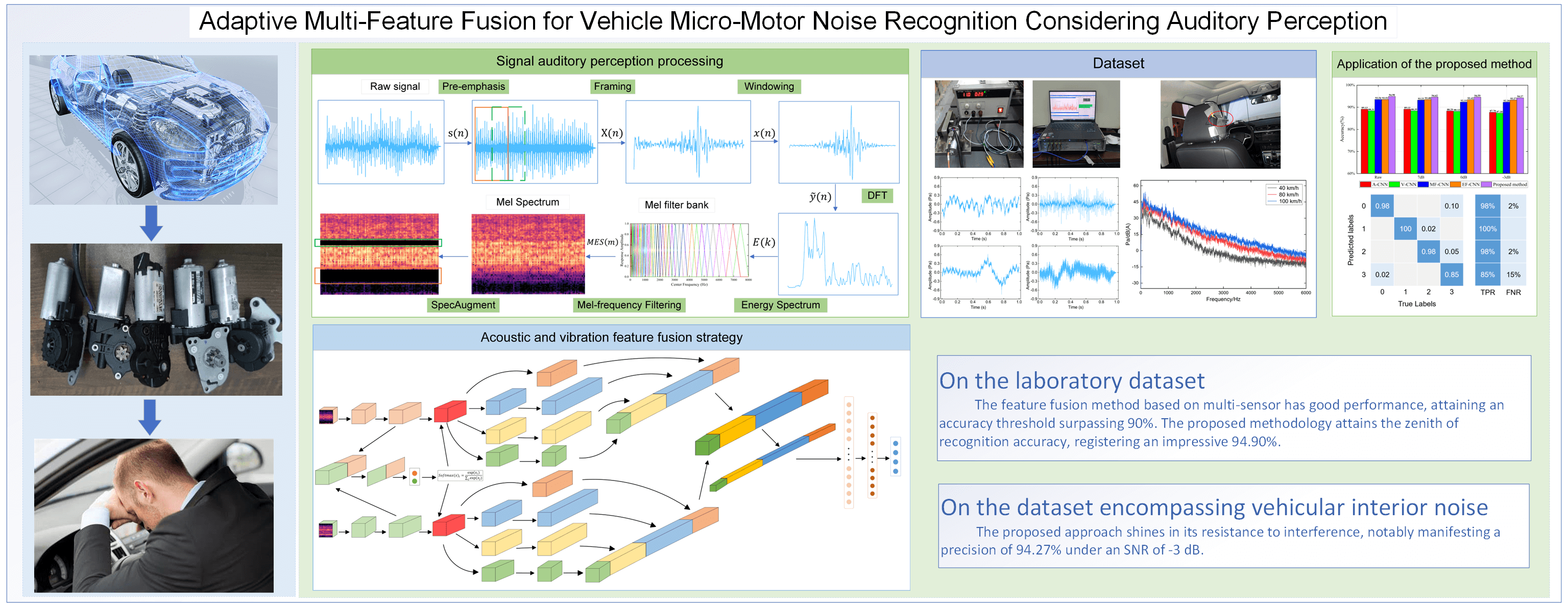
The deployment of vehicle micro-motors has witnessed an expansion owing to the progression in electrification and intelligent technologies. However, some micro-motors may exhibit design deficiencies, component wear, assembly errors, and other imperfections that may arise during the design or manufacturing phases. Consequently, these micro-motors might generate anomalous noises during their operation, consequently exerting a substantial adverse influence on the overall comfort of drivers and passengers. Automobile micro-motors exhibit a diverse array of structural variations, consequently leading to the manifestation of a multitude of distinctive auditory irregularities. To address the identification of diverse forms of abnormal noise, this research presents a novel approach rooted in the utilization of vibro-acoustic fusion-convolutional neural network (VAF-CNN). This method entails the deployment of distinct network branches, each serving to capture disparate features from the multi-sensor data, all the while considering the auditory perception traits inherent in the human auditory system. The intermediary layer integrates the concept of adaptive weighting of multi-sensor features, thus affording a calibration mechanism for the features hailing from multiple sensors, thereby enabling a further refinement of features within the branch network. For optimal model efficacy, a feature fusion mechanism is implemented in the concluding layer. To substantiate the efficacy of the proposed approach, this paper initially employs an augmented data methodology inspired by modified SpecAugment, applied to the dataset of abnormal noise samples, encompassing scenarios both with and without in-vehicle interior noise. This serves to mitigate the issue of limited sample availability. Subsequent comparative evaluations are executed, contrasting the performance of the model founded upon single-sensor data against other feature fusion models reliant on multi-sensor data. The experimental results substantiate that the suggested methodology yields heightened recognition accuracy and greater resilience against interference. Moreover, it holds notable practical significance in the engineering domain, as it furnishes valuable support for the targeted management of noise emanating from vehicle micro-motors.Graphic Abstract
Keywords
The progressive surge in the integration of micro-motors within vehicles, encompassing components such as wipers, seat adjusters, and lifting glass motors, epitomizes the overarching trajectory towards vehicle electrification and enhanced intelligence [1,2]. Moreover, the functionalities attributed to these vehicular micro-motors have evolved into a realm of heightened diversity and intelligence [3]. Notably, electric vehicles, distinguished by their absence of exhaust emissions and engine noise, entail lower levels of interior noise in contrast to their combustion-engine counterparts [4]. Nonetheless, a distinct shift has been observed, whereby the prominence of interior micro-motor noise within vehicles has become increasingly perceptible [5]. Pertinently, certain micro-motors may be susceptible to design imperfections, component deterioration, assembly discrepancies, and other anomalies encountered across the design and manufacturing continuum, thus engendering the manifestation of aberrant acoustic emissions during their operational phases [6]. The architectural landscape of vehicle micro-motors has embraced a realm of diversification [7], consequently giving rise to a proliferation of intricate aberrant auditory manifestations, mandated by the necessity to harmonize within the spatial confines of the vehicular interior whilst accommodating an array of functional requisites. The genesis of noise emanating from vehicle micro-motors is rooted in a multifarious interplay of sources, a confluence modulated by their distinctive structural attributes, operational tenets, and inherent characteristics. The composite constitution of micro-motors typically encompasses constituent elements such as the rotor, stator, bearing, and gear, among others. Each such component may be vulnerable to an assortment of issues, encompassing bearing and gear wear, mechanical slackening, design deficiencies inherent to the micro-motor, and the incitation of shell vibrations attributable to electromagnetic forces.
Owing to the heterogeneous spectrum of abnormal noise typologies, conventional methodologies predicated on manual feature extraction and classification algorithms are intrinsically limited in their capacity to encompass the entirety of aberrant auditory variations. In stark contrast, deep learning has emerged as a formidable paradigm, leveraging intricate neural architectures to hierarchically extract salient attributes from input data, obviating the necessity for labor-intensive manual feature extraction processes [8]. Each stratum of non-linear activation functions within the intricate fabric of deep neural networks augments their expressive potency, affording robust learning capabilities and adaptability. Techniques grounded in deep learning have garnered widespread acclaim across diverse domains such as acoustic recognition, damage localization [9,10], and anomaly discernment [11,12], underscoring their efficacy. To capture the nuances of noise characteristics manifesting within diverse noisy contexts, Cha et al. [13] unveiled an active noise control (ANC) paradigm predicated on feedback loops, harnessed through the prism of deep learning. Kim et al. [14] harnessed a variational autoencoder (VAE) to distill the parameters underpinning vehicular-generated buzzing, squeaking, and rattling (BSR) noise. Meanwhile, Choudhary et al. [15] devised a multi-input convolutional neural network, evincing remarkable accuracy across diverse operational scenarios for bearing and gear datasets. An indispensable facet of the deep learning repertoire is encapsulated by the convolutional neural network (CNN). Renowned for its prowess in effectuating feature extraction, CNN has pervaded an array of applications encompassing fault diagnosis [16,17], acoustic profiling [18,19], and diverse other domains. Its adeptness in discerning patterns, even within the confines of intricate settings [15,20] and challenging contexts, has been unequivocally established. Nonetheless, conventional CNN architectures may inherently fall short of meeting the multifarious prerequisites intrinsic to micro-motor abnormal noise classification. In a concerted endeavor to fortify the feature extraction potential of the neural network paradigm and consequently enhance classification accuracy, the present research introduces an elevated iteration of CNN, ingeniously integrating Inception modules.
Certain micro-motors, such as the headrest motor embedded within electric seats, often reside in close proximity to the human auditory organ, rendering their auditory perception notably discernible. These micro-motors are intricately linked with numerous vehicular components, thereby engendering a multitude of dispersed noise sources that collectively yield substantial acoustic emissions. The advent of abnormal noise engenders discomfort and agitated emotions in both drivers and passengers, thus detrimentally impacting their overall comfort and ride experience. Notably, a fundamental disjunction exists between human auditory perception and the generation of sound, stemming from the distinct processes governing auditory reception and sonic generation, which underscores the role of the human auditory system in sound perception. To align with the intricacies of human acoustic perception, the Mel spectrum adopts Mel filters to effectuate a non-linear frequency band division, thereby mirroring the human auditory apparatus more faithfully. Rooted in the tenets of human auditory cognition, the Mel spectrum aptly lends itself to noise analysis, demonstrating resilience against extraneous noise and data gaps during transformation. Within the realms of audio processing [21,22] and vocal recognition [23–27], the Mel spectrogram has been pervasively and efficaciously employed. Furthermore, select inquiries have progressively integrated Mel features into the realm of sound event detection and classification, encompassing machinery noise [28,29] and environmental acoustics [30]. Shan et al. [31] judiciously merged Variational Mode Decomposition (VMD) with the Mel spectrogram to discern motor bearing anomalies. Tran et al. [32] adroitly harnessed the Mel spectrogram to classify authentic noise emanating from industrial drilling apparatus. Abeysinghe et al. [33] harnessed Mel Frequency Cepstral Coefficients (MFCC) as pivotal feature data, augmented by ancillary statistical indices, for the identification of vehicular malfunction sounds. Gong et al. [34] leveraged MFCC to gauge the vehicular powertrain system’s condition. Wang et al. [35] adeptly employed the Mel spectrogram to diagnose engine acoustic aberrations. Engineering praxis has underscored the efficacy of preprocessing methodologies grounded in auditory perception, endowing a novel avenue for discerning irregular noise emanations within micro-motors embedded within vehicular domains.
Ordinarily, the acquisition of abnormal noise signals necessitates the deployment of either a sound pressure sensor, a vibration acceleration sensor, or a displacement sensor. Nevertheless, the utilization of solitary sensor data remains inadequate for the comprehensive and precise encapsulation of the intricate characteristics underpinning micro-motor abnormal noise within real-world contexts, owing to the diverse array of loads and extraneous acoustic influences at play. Moreover, this monosensory approach is susceptible to signal attenuation, environmental perturbations, and assorted extrinsic variables, thereby impinging upon the overall resilience and fidelity of the endeavor to identify abnormal noise manifestations [36]. Through the strategic amalgamation of features culled from an assortment of sensors, the capacity to discriminate amongst multifaceted variants of abnormal noise in vehicular micro-motors [37,38] is facilitated, concurrently affording the opportunity to glean supplemental insightful data points from a multiplicity of sensor sources.
In preceding investigations, the approach of extracting features from individual sensors through the utilization of Convolutional Neural Networks (CNNs) has demonstrated efficacy in fault diagnosis, speech recognition, and analogous domains. However, within the realm of noise identification concerning vehicle micro-motors, particularly those characterized by intricate and diverse configurations and functionalities, a rudimentary CNN architecture encounters challenges in meeting the multifarious demands inherent to this context. Limited research endeavors have accounted for the amalgamation of multi-sensor features in the context of auditory perception. Consequently, this study introduces a signal preprocessing methodology for auditory perception that incorporates the subjective auditory discernment of abnormal noise by vehicle micro-motors from the vantage point of the driver and passengers. Furthermore, the proposed methodology adopts a multifaceted sensor feature fusion technique, culminating in the derivation of features akin to those perceptible to the human auditory apparatus. This article proffers an innovative noise identification paradigm for vehicle micro-motors, predicated on the fusion of multiple features, while aptly considering auditory perception. In juxtaposition to alternative methodologies, the proposed approach adeptly ascertains the adaptive weighting and fusion of the derived multifaceted features, in alignment with the auditory responsiveness of the human ear. Additionally, this approach effectively manages the influence of ambient noise, robustly exhibiting superior anti-interference capacities.
The principal contribution of this paper lies in the proposition of an adaptive multi-feature fusion methodology tailored to the identification of abnormal noise emanating from vehicle micro-motors, while simultaneously considering the tenets of auditory perception. Within this study, the formulated approach is deployed for the recognition of an abnormal noise dataset associated with vehicle micro-motors, garnered through laboratory experimentation. Comparative analyses are subsequently conducted to assess the recognition efficacy of the models. Furthermore, an appraisal of the model’s resilience against interference is performed using a dataset encompassing interior vehicular noise.
The rest of the paper is organized as follows: Section 2 introduces the proposed method, suggests the VAF-CNN model, describes the auditory perception signal preprocessing method, and explains the multi-feature adaptive weighting approach. The experiment and dataset construction are described in Section 3. The results and discussion of the model performance evaluation are presented in Section 4. The conclusion is provided in Section 5.
2 Multi-Sensor Adaptive Feature Fusion Method Based on Auditory Perception
2.1 Multi-Sensor Feature Fusion Model (VAF-CNN)
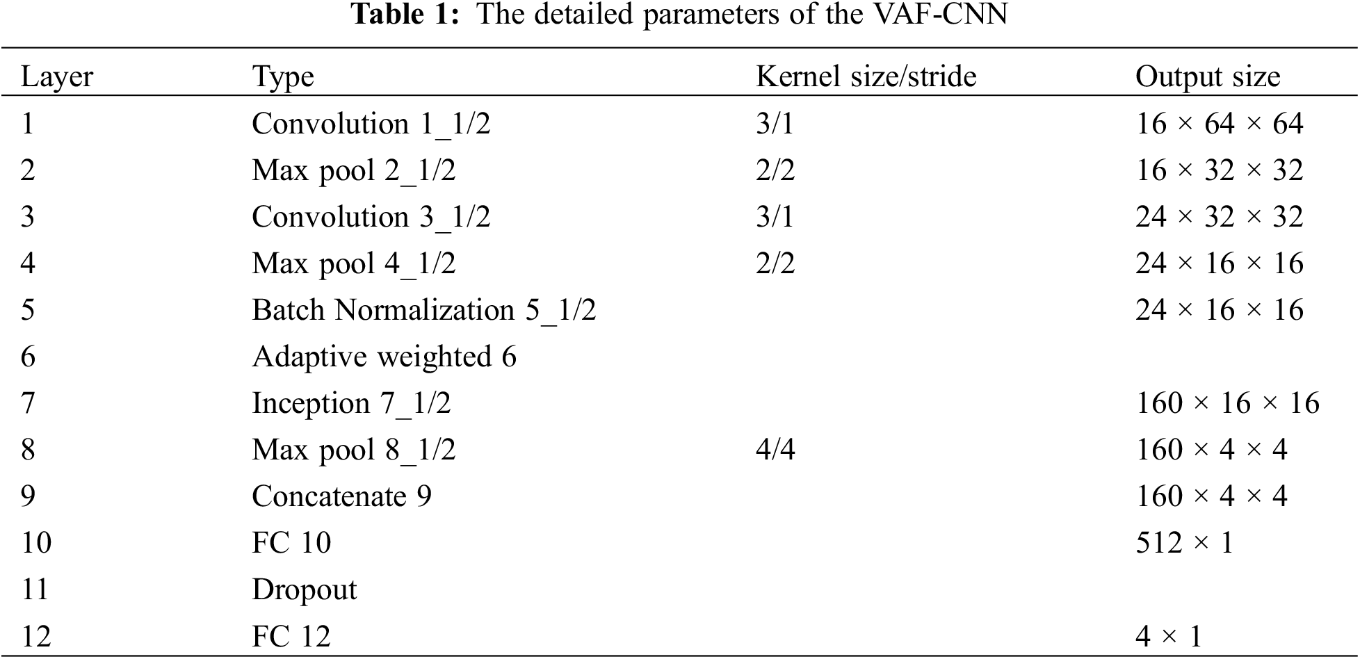
The identification of abnormal noise in vehicle micro-motors is addressed in this paper using a multi-sensor feature adaptive fusion approach based on auditory perception and using acoustic and vibration signals as inputs. The method generally consists of four stages: feature fusion, multi-scale feature extraction, sensor feature weighting, and feature extraction from different scales. First, branch network CNN is used to extract features from various sensor data; after that, a feature adaptive weighting layer is used to calibrate the extracted features; next, the Inception module is used to extract multi-scale features separately; and finally, two branch network features are fused, and the fused features are input to the fully connected layer for classification. The framework diagram of the proposed model for fusing multi-sensor features is shown in Fig. 1 and the parameters of the VAF-CNN are detailed in Table 1.
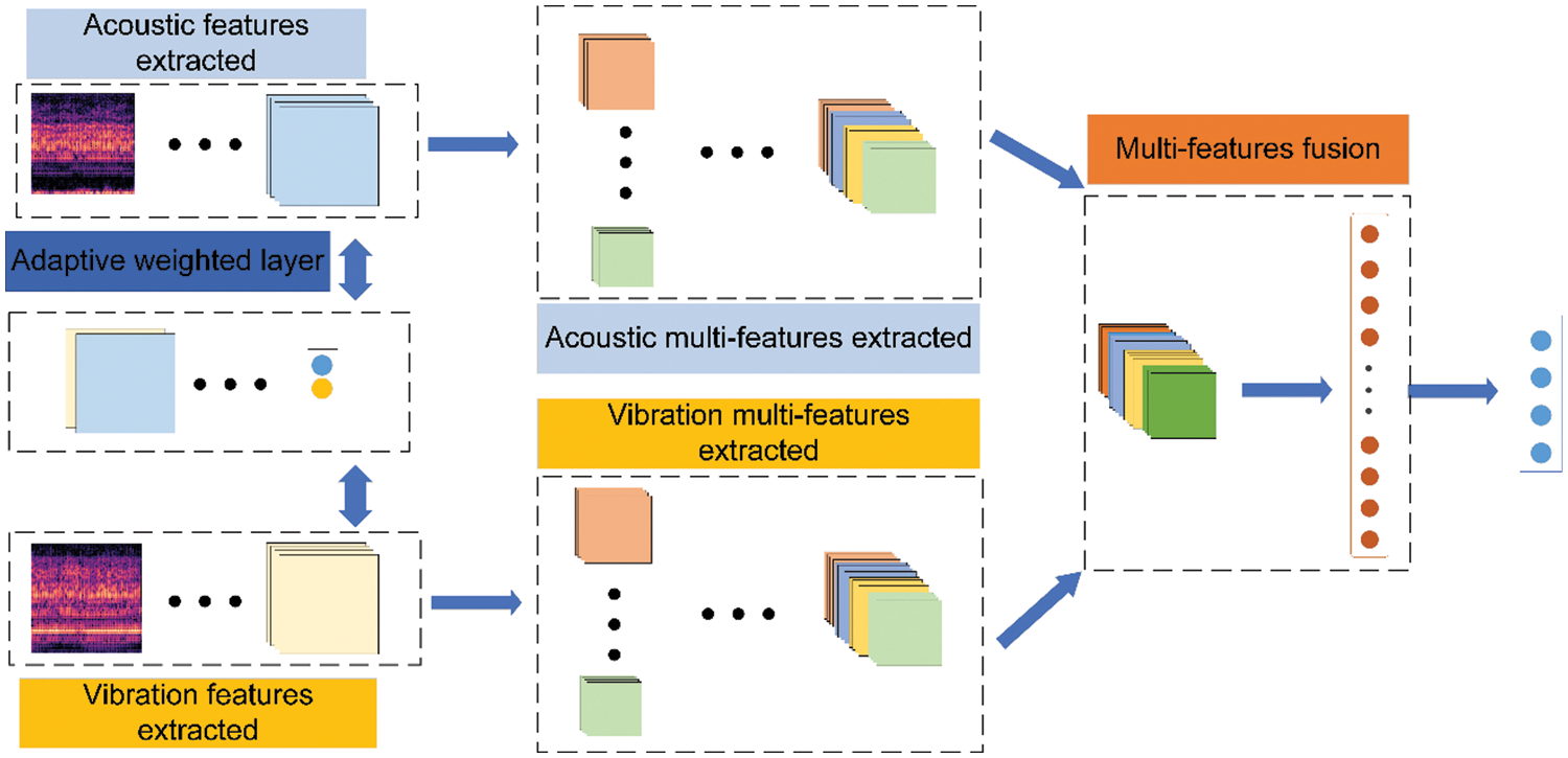
Figure 1: The schematic architecture of the VAF-CNN
CNN (Convolutional Neural Network) is a feed-forward multilayer neural network model consisting of convolutional, pooling, and fully connected layers. It involves linear and nonlinear operations and has powerful fitting abilities. In this paper, CNN is used to extract the features of the sensor.
Convolution layer: the convolution kernel of the convolution layer has the characteristics of weight sharing and translation invariance, which enhance the ability of feature extraction. The output of the convolution layer is mapped by the activation function; in this paper, we use the ReLU activation function. Its mathematical expression is as follows:
where
Pool layer: two common pooling methods are maximum pooling and average pooling. In this paper, only the Inception module uses the average pooling, while other places use the maximum pooling. The maximum pooling mathematical expression is:
where
Fully Connected Layer: Fully connected layers are typically used to combine feature vectors, further extract features, and perform classification operations. In the fully connected layer, each neuron is connected to all the neurons in the adjacent layers, which leads to a huge number of parameters, therefore, in this paper, we use Dropout after the first fully connected layer with a random dropout rate of 0.5. The mathematical expression for the fully connected layer is:
where
Batch Normalization: This paper uses batch normalization to standardize the input features of different sensors as the standard normal distribution, to avoid the phenomenon of internal covariate shift and gradient vanishing in the network forward propagation, and to speed up the model convergence. Its mathematical expression is as follows:
where
Inception [39] is a special CNN structure with characteristics of different convolution and parallel structures. In this paper, multiple parallel convolution layers and a pooled layer are used to extract different noise features at different scales by convolution of multiple parallel branches. The 1 × 3, and 5 × 1 convolution kernels are used to obtain different sizes of receptive fields, respectively, to increase the richness of feature extraction and improve the feature extraction capability of the model. In addition, to reduce the number of parameters and computational complexity, the 1 × 1 convolution kernel is subjected to dimensionality reduction and dimensionality enhancement operations. The specific parameters of the Inception module in this paper are shown in Fig. 2.
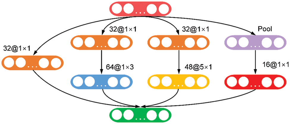
Figure 2: Inception layer used by the VAF-CNN
2.2 Signal Acoustic Perception Processing
The spectrogram representation known as the Mel spectrum is excellent at capturing the sound that the human auditory system hears. To create the Mel spectrogram, the frequency axis is divided into many isometric intervals, and the energy values within each interval are added together. Fig. 3 depicts the Mel spectrum extraction procedure.
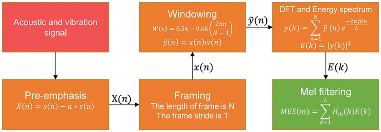
Figure 3: The Mel spectrogram extraction process
(1) Pre-emphasis. The pre-emphasis is applied to the acquired signal to enhance the high-frequency components of the signal with a high-pass filter. In this paper, the pre-emphasis coefficient is 0.97. The transfer function of the high-pass filter can be expressed as:
where
(2) Framing. Considering the short-term stationarity of the signal, it is necessary to perform a sub-framing operation on the signal and ensure that there is a partial overlap between adjacent frames to avoid frequency leakage. In this paper, the frame length is set to 25 ms, and the frameshift is set to 15 ms. The framing is illustrated in Fig. 4.
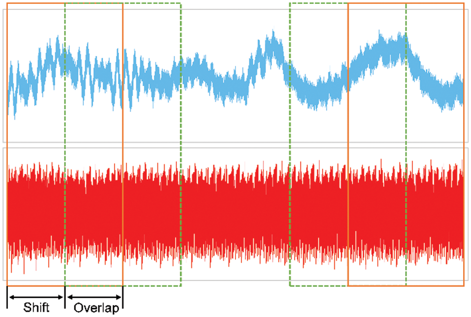
Figure 4: Signal framing process
(3) Windowing. Windowing is performed on each frame of data to increase the continuity between the two ends of the frame, thereby reducing the spectrum leakage and sidelobe size in the process of FFT conversion. In this paper, the Hamming window is used as the windowing function, and its expression is as follows:
where
(4) Discrete Fourier Transform (DCT). The Discrete Fourier Transform is performed on the windowed signal to obtain the spectrum. The formula for the transformation is as follows:
where
(5) Mel filter bank. After the spectrum of the signal is obtained, the Mel filter is used to filter the spectrum, the energy of the filter bank is calculated, and then the MEL spectrum is generated. The relationship between the Mel scale and linear frequency f is shown in Eq. (10), the Mel filter is shown in Fig. 5, the calculation formula is shown in Eq. (11), and the Mel energy filtered by the filter is shown in Eq. (12).
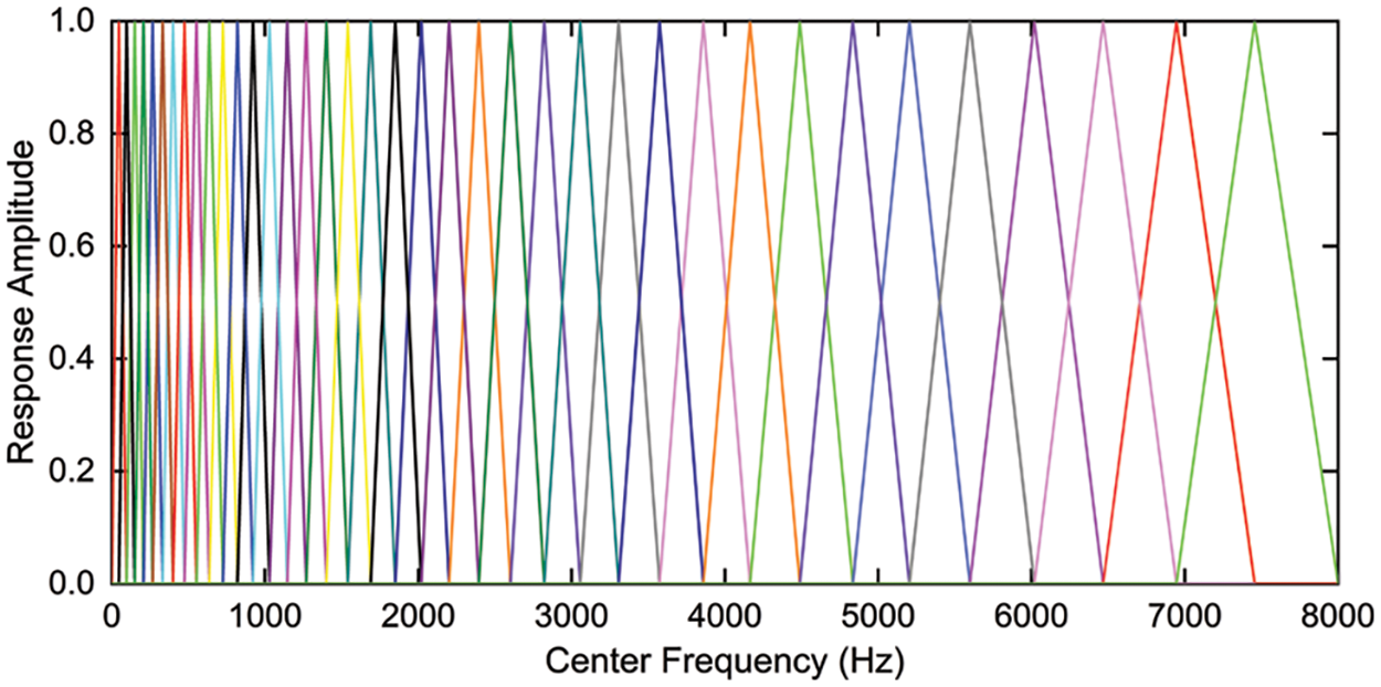
Figure 5: Mel filter bank
where
(6) SpecAugment-based data augmentation. A data augmentation approach called SpecAugment [40] analyses signal from a visual perspective and employs time warping, frequency masking, and time masking strategies. It is frequently used in voice and audio processing. This paper selects a frequency masking method because the characteristics of the various noise parts in this work show good consistency in the time domain but a significant gap in the frequency domain. In order to guarantee incomplete masking of the feature frequency band, the frequency masking approach is enhanced in accordance with the noise characteristics. To simulate samples with partially missing frequency information, localized masking zones are created. The frequency masking strategy for SpecAugment is: The frequency dimension is masked so that
1) Selection of masking frequency range [0, 4200 Hz];
2) The number of frequency blocks selected for use is 2. The Mel frequency band is nonlinearly and evenly divided, and the lower the frequency, the denser the Mel frequency band. Therefore, two consecutive Mel frequency channels are set, and the frequency channels range is [0,1000 Hz] and [1000, 4200 Hz];
3) The random masking parameters
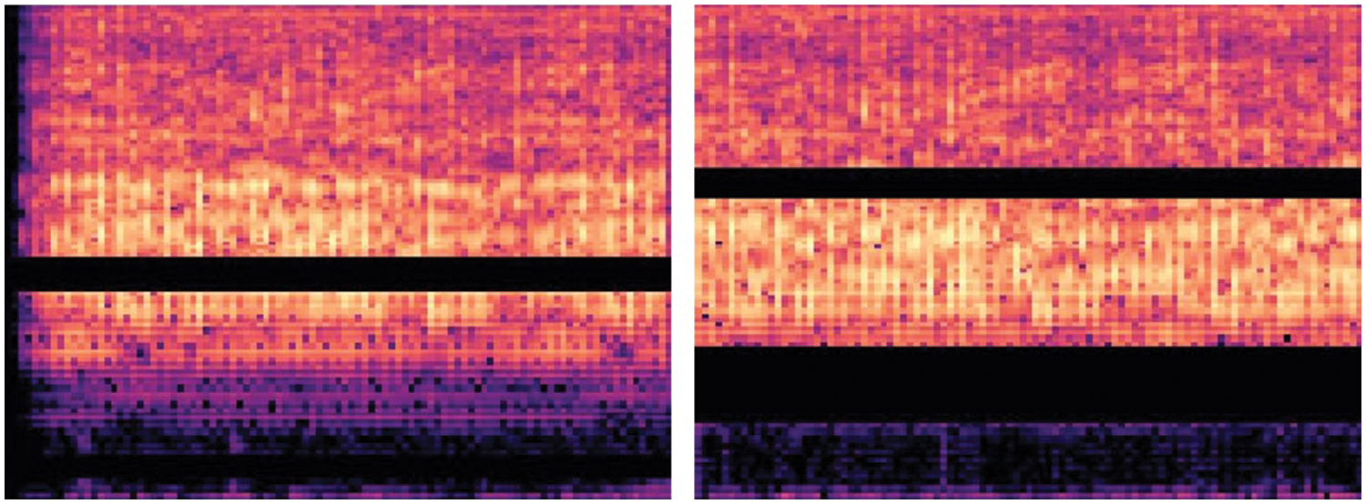
Figure 6: The Mel spectrogram masking by improved data augmentation method
2.3 Multi-Sensor Feature Adaptive Weighting Method
The features that are extracted from the data from multiple sensors are redundant and correlated. The fusion of various signals and signal features is typically accomplished using traditional data fusion approaches, which either manually calculate the weights required or simply combine features for fusion before inputting them into the deep structure to extract representative features for recognition. However, mutual interference between different signal types becomes particularly noticeable when signals of the same type are fused, leading to the model’s extraction of several duplicate features. Additionally, the presence of significant features may be lost due to the blurring of sensor data features. The traditional weight assignment approach requires prior knowledge, the weight obtained is not always applicable to the input data currently being used, and it is not possible to automatically alter the weight to take into account new data.
In order to address these problems, a multi-sensor feature-adaptive weighting method is presented. This method can calculate the weight of a sensor based on the data’s feature distribution, effectively balancing the redundancy and correlation between various sensor features and improving the accuracy and stability of the feature extraction process. Using the vibration signal and the acoustic signal as examples, the Mel spectrograms of the various sensors are first input into the two branch networks, where the depth features of the data from a single sensor are automatically extracted. Next, the features of the multiple sensors are weighted.
Let
1) Use the global average pooling operation to compress the spatial dimension of different sensor signals’ features:
where
2) Combine the compressed features of two sensor signals to generate a global representation. Additionally, introduce fully connected operations to improve nonlinearity:
where
3) Based on the compression feature
where
4) Recalibration or fusion of features from different sensor data through a gating mechanism:
where
3.1 Abnormal Noise Acquisition Experiment
All of the motors utilized in this experiment are micro-motors within the vehicle, and Fig. 7 illustrates some typical motor types. The acquisition experiment was conducted in a semi-anechoic chamber with minimal environmental noise. Online collecting, analyzing, and processing were done in the experiment using a 48-channel LMS SCADAS Mobile front-end data acquisition system from Siemens and the Signature Testing-Advanced module of Simcenter Testlab2021 software. The three-way vibration sensor (model: B05Y32) and the BSWA sound pressure sensor (model: MA231-570434) were both utilized for collecting vibration and acoustic signals, respectively. To replicate the fixed position of the motors on a real vehicle, the vehicle’s micro-motors were all fixed to the corresponding fixture. The sound pressure sensor and vibration sensor took samples while the micro-motor was running. The vibration sensor was attached to the motor shell, and the sound pressure sensor was 50 cm away from the micro-motor. The field experiment is shown in Fig. 8.
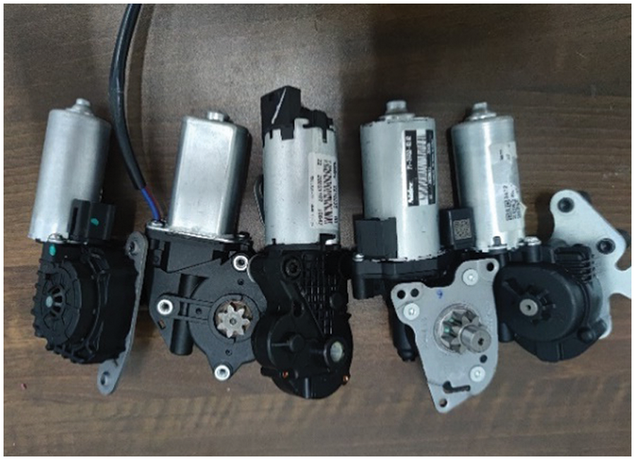
Figure 7: Different types of micro-motors for vehicles
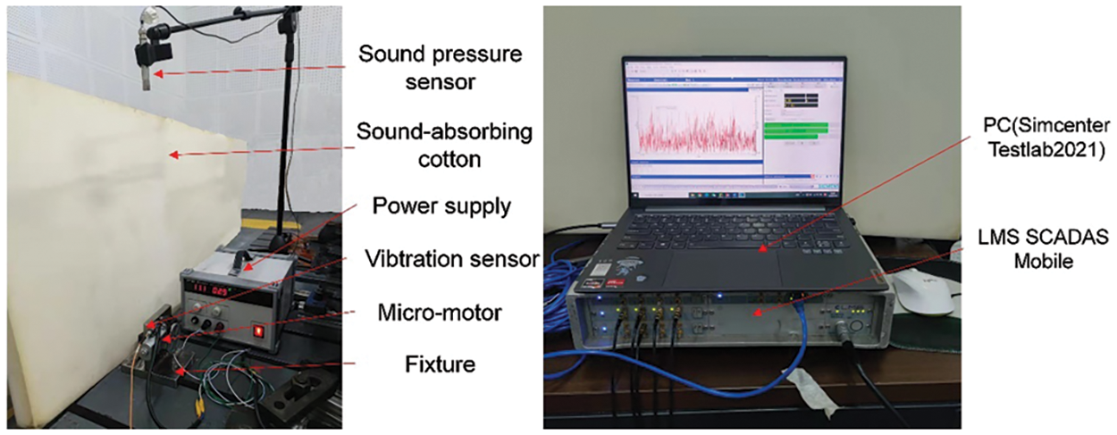
Figure 8: Vehicle micro-motor noise acquisition system
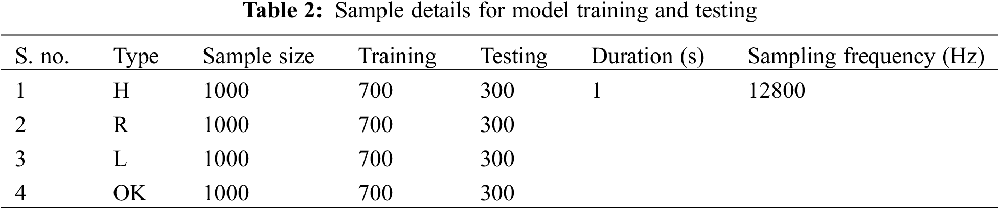
The resolution is 1 Hz, while the sampling frequency for acoustic and vibration signals is 12800 Hz. To assure the accuracy of the micro-motor sample labels, the acquisition procedure used samples of abnormal micro-motor noise supplied by a corporation, and the running micro-motor noise was manually labeled by professional technicians. This paper chooses four types of abnormal noise with lower BI index values and a higher frequency of occurrence as the research objects. This selection was made in accordance with the BI index and frequency of occurrence of micro-motor products offered by a manufacturer. The customer’s subjective assessment of the motor’s noise is reflected in the BI index, and the lower the value, the worse the subjective feeling.
Two different noise datasets were used in this paper: the first one is a dataset without vehicle interior noise, and the second is a dataset with vehicle interior noise. Road noise, wind noise, and drive motor noise are only a few examples of the inherent environmental characteristics that contribute to the interior noise of vehicles in motion. By including vehicle interior noise, the micro-motor application scenario can be more accurately simulated, and the model can be exposed to more real and complex sound scenes during the training process, allowing for an evaluation of the proposed method’s applicability in the real-world driving environment.
The first kind of dataset is built from laboratory samples, with each sample lasting 1 s and each signal receiving 1000 samples for a total of 4000 samples. Fig. 9 displays the time-domain waveforms of the four different types of noise. The dataset details are shown in Table 2.
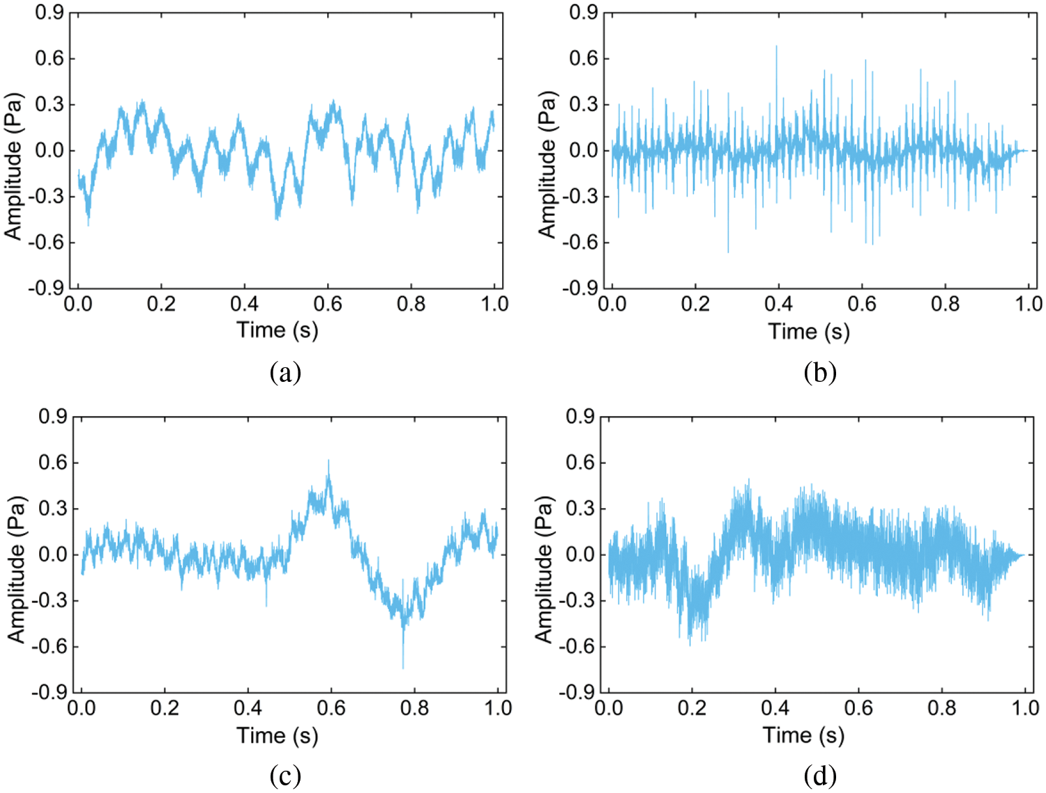
Figure 9: The acoustic time-domain signals of four abnormal noise of vehicle micro-motor, (a) H, (b) R, (c) L, (d) OK
The interior noise of an electric vehicle is chosen for the second type of dataset construction. Asphalt is used as the test surface, and the test conditions included uniform speeds of 40, 80, and 100 km/h. Right behind the driver’s right ear is the sound pressure sensor. Fig. 10 displays the noise spectrum diagram of the acquired vehicle interior.
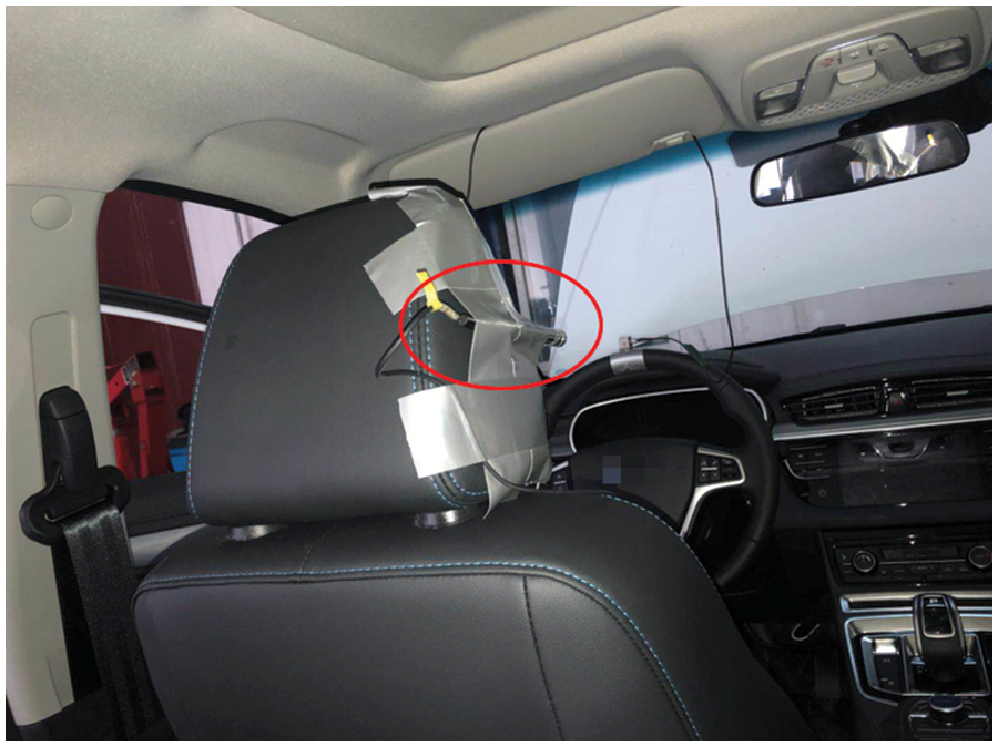
Figure 10: Driver’s right ear noise measurement point of the test vehicle
In order to construct the second type of dataset, an electric vehicle was selected to collect the interior noise. The test location was an open road in Chengdu, and the operating condition for internal car noise was chosen to be constant speed. There were three constant speeds: 40, 80, and 100 km/h. The right ear of the driver served as the location of the sound pressure sensor, and the test duration was longer than 5 s with a 25600 Hz sampling frequency. Fig. 11 displays the noise spectrum diagram of the acquired vehicle interior.
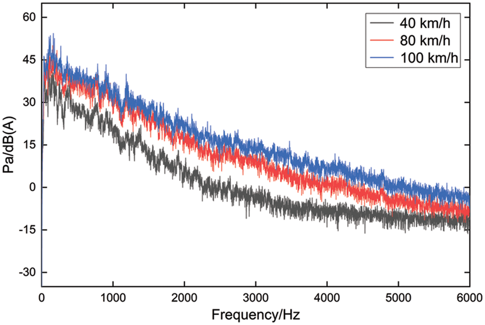
Figure 11: Noise spectrum of the test vehicle at different speeds
To replicate the use of the micro-motor on a real vehicle, the interior noise of the vehicle at 40, 80, and 100 km/h was superimposed on the laboratory dataset. The specific superposition method is as follows: the interior noise of the vehicle is downsampled, and the signal is intercepted to ensure that the interior noise of the vehicle and the abnormal signal have the same sampling rate and length. Then, the two signals are added at each sampling point, and the signal after superposition is obtained. The signal-to-noise ratio (SNR) [41] is a frequently employed quantitative index to assess the relative intensity between the signal and the interior noise in a vehicle. The interior noise in the vehicle will interfere with the original signal. The lower SNR is a symptom of increased signal interference and louder noise. Therefore, the vehicle interior noise and the original signal at different speeds are calculated according to the SNR calculation formula, which is provided in Eq. (21), to evaluate the level of influence of vehicle interior noise at different speeds on different noises. The SNR is 7, 0, and −3 dB at 40, 80, and 100 km/h, respectively.
where
4 Analysis and Discussion of Results
On a noise dataset without interior noise and a noise dataset with interior noise, respectively, recognition experiments are conducted to evaluate the performance of the proposed approach and its application in a real driving situation. The neural network is trained on 70% of the sample from the dataset, while it is tested on the remaining 30%. The training model for the neural network is created using the acoustic and vibration sensor data from the training samples. Following the entry of the test samples into the trained model for testing, the output results of the model based on single-sensor data and those of other models based on multi-sensor data are compared.
4.1 Model Evaluation and Comparison
In this section, the proposed VAF-CNN is experimented with on two datasets to illustrate the applicability of the suggested approach, first contrasting it with the results of previous feature fusion models based on multi-sensor data and subsequently with results from single-sensor data. The feature fusion model accepts data from both vibration and acoustic sensors, unlike single-branched networks, which only accept data from a single sensor. In Fig. 12, the comparative model is displayed. For multi-class classification problems, confusion matrices are used to evaluate, quantify, and visualize the performance of classifiers. The performance parameters of the classifier are calculated using the following relationships:
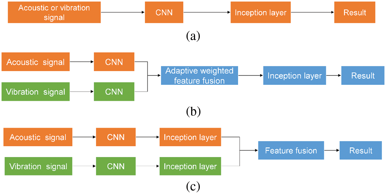
Figure 12: Single-sensor and multi-sensor method framework, (a) A-CNN (Acoustic)/V-CNN (Vibration), (b) MF-CNN, (c) EF-CNN
where TP is the true positive samples, TN is the true negative samples, FP is the false positive samples, and FN is the false negative samples.
(a) A/V-CNN (CNN for acoustic or vibration sensor data input.) The model takes acoustic or vibration sensor data as input, does not include the BN layer and feature fusion layer, and only uses a fully connected layer. In addition, the other layers are the same as the single-branch network of the proposed method.
(b) MF-CNN (CNN model for fusing acoustic and vibration sensor features at the middle layer) This model takes acoustic and vibration sensor data as input, and multi-sensor features are adaptive weighted fusions in the middle layer.
(c) EF-CNN (CNN model for fusing acoustic and vibration sensor features at the last layer) This model takes acoustic and vibration sensor data as input, and there is no multi-sensor feature adaptive weighting layer in the middle layer, and only simple feature fusion is carried out in the last layer.
The results of VAF-CNN were compared with those of other models. Both the proposed model and the comparison model were run 10 times, and their average prediction accuracy was taken as the final measure. The implementation of the model uses the Pytorch framework and is built in the Python language. The initial learning rate of the model is 0.001, the loss function is cross-entropy loss, the optimization algorithm is the Adam algorithm, the regularization is L2 regularization, and the weight attenuation is 0.001. The model training is carried out in small batches. The number of samples sent to the network is 128 each time, and the input size of images is 64 × 64.
Table 3 displays the average prediction accuracies of the aforementioned models for 10 runs on both datasets. On the lab dataset, the single-sensor models all have accuracy levels below 90%, while the accuracy of the model results of multi-sensor feature fusion is greater than the accuracy of a single sensor, and the accuracy of VAF-CNN is the greatest, reaching 94.90%.
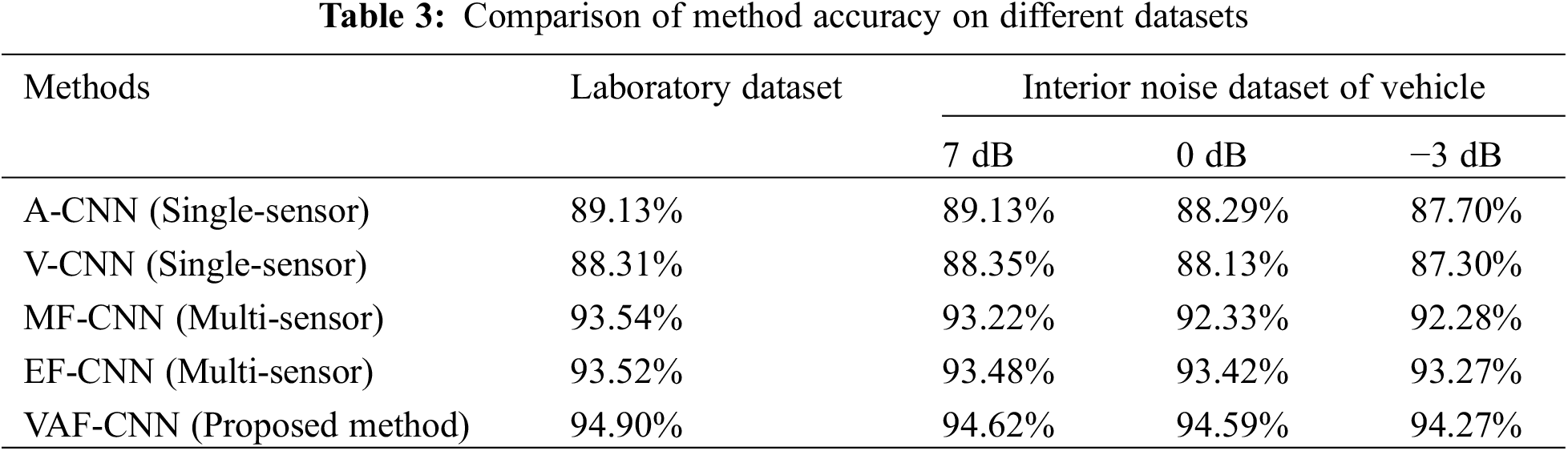
On the dataset containing vehicle interior noise with an SNR of 7 dB, the accuracy of all models performs well. The single-sensor model and the multi-sensor feature fusion model both exhibit some anti-interference ability at high SNR. With a VAF-CNN accuracy of 94.62%, the multi-sensor feature fusion model is more accurate.
On the dataset containing vehicle interior noise with an SNR of 0 dB, the accuracy of single-sensor models decreases, all of them are lower than 89%, among which the accuracy of the A-CNN model decreases more; the accuracy of the multi-sensor feature fusion model also decreases, among which the accuracy of the MF-CNN decreases the most, and the accuracy of the VAF-CNN model is 94.59%.
The accuracy of the single sensor model drops to less than 88% on the dataset containing vehicle interior noise with an SNR of −3 dB, and the V-CNN model drops the most. The accuracy of the VAF-CNN is 94.27%, and the accuracy of the multi-sensor feature fusion model is greater than 92%.
In the single sensor model, the accuracy of A-CNN is higher, and the anti-interference capacity of V-CNN is stronger, with a 1.01% accuracy drop as SNR lowers. In the multi-sensor feature fusion model, VAF-CNN has the maximum accuracy with a decreasing signal-to-noise ratio, whereas MF-CNN has worse anti-interference capabilities and its accuracy drops by 1.26%.
The results of the multi-sensor feature fusion model outperform those of the single sensor model in that their overall accuracy is higher than 92%, their anti-interference ability is stronger, and their accuracy declines range from 0.25% to 1.26%. The anti-interference capabilities of EF-CNN and VAF-CNN are superior to those of the multi-sensor feature fusion model, and VAF-CNN has the highest overall accuracy.
The results of the other classification indicators for the five models mentioned above are listed in Tables 4–7. The model with multiple sensors as input performs better and has better evaluation indices than the A-CNN and V-CNN models with a-single sensor as input. The VAF-CNN model performs better in classification compared to MF-CNN and EF-CNN with multiple sensors as input.
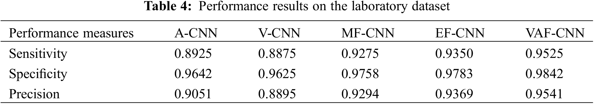
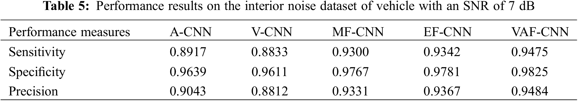
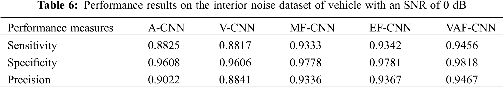
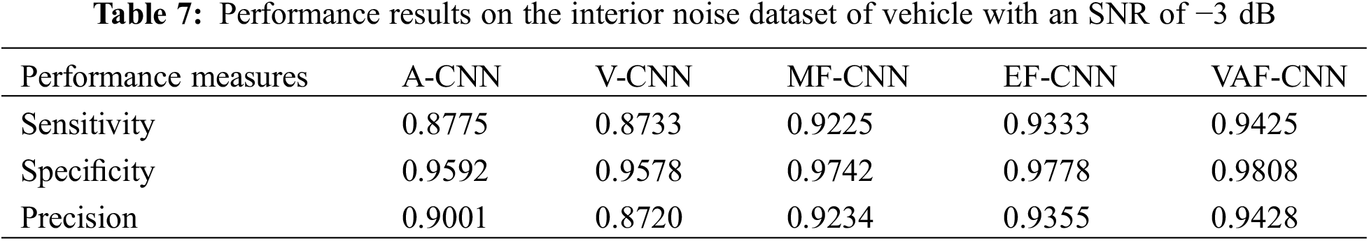
Fig. 13 displays the predicted confusion matrix for the five models on the laboratory dataset. The confusion matrix’s vertical axis denotes the sample’s expected label, the horizontal axis denotes the actual label, the diagonal line denotes the percentage of correct classifications, and the non-diagonal elements denotes the percentage of incorrect classifications. The confusion matrix visually shows the model’s performance in identifying different classes of samples and provides a more specific evaluation of performance metrics through true positive (TPR) and false negative rates (FNR). By utilizing the true positive rate and false negative rate, it becomes possible to determine the percentage of samples correctly identified as belonging to their respective categories, as well as the percentage of samples incorrectly classified as belonging to other categories.
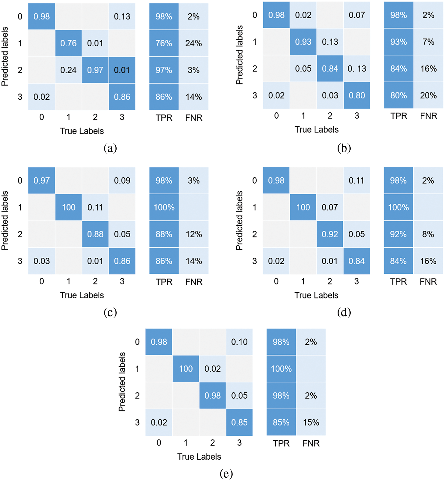
Figure 13: The confusion matrix of the result for the test samples on the laboratory dataset, (a) A-CNN, (b) V-CNN, (c) MF-CNN, (d) EF-CNN, (e)VAF-CNN
The overall differentiation of VAF-CNN is stronger in comparison to the model with a single sensor as input (Figs. 13a and 13b), and the classification effect on labels 1 and 2 is better than that of the single sensor data model. With only a 0.02 misclassification rate on label 2, VAF-CNN outperforms other multi-sensor feature fusion models (Figs. 13c and 13d), and its overall classification result is the best. Compared to the model with a single sensor as input, the feature fusion model with multiple sensors as input is able to select the features of a single sensor and realize feature complementarity, thus improving the classification accuracy of the model.
To intuitively understand the capabilities of the proposed VAF-CNN in feature extraction and classification, t-SNE [42] is used to map high-dimensional data into a low-dimensional space for visualization. Fig. 14 displays the visualization results for the input layer, feature extraction layer (Max pool 8_1/2), feature fusion layer (Concatenate 9), and fully connected layer (FC 10) of the VAF-CNN network model used in this paper.
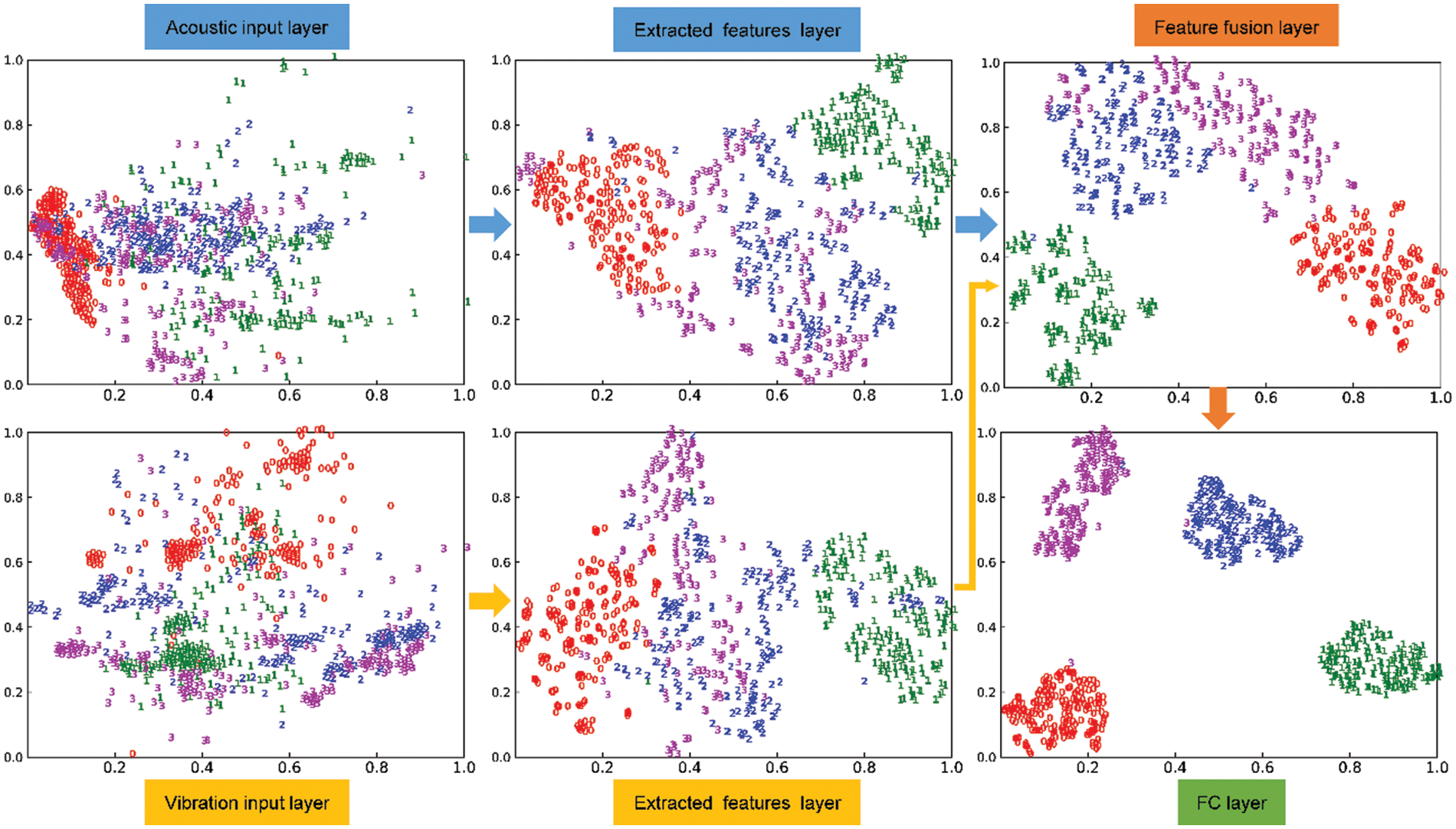
Figure 14: Feature visualization of the VAF-CNN
Fig. 14 shows that the data samples for the four different types of labels are entirely mixed together in the multi-sensor data input layer, with labels 0 and 3 and labels 1 and 2 having some overlap. Labels 0 and 3 overlap more visibly in the acoustic signal input layer, suggesting that labels 1 and 2 and labels 0 and 3 are similar and that it is challenging to identify them apart.
Labels 0 and 1 can be distinguished after two branches of extracted features, showing that they can be identified by using single-sensor acoustic or vibration data as input. However, there is still some overlap between labels 1 and 2, as well as between labels 0 and 3, showing that their differentiation is relatively poor. This agrees with the A/V-CNN model’s results for the confusion matrix.
Labels 2 and 3 are differentiated in the feature fusion layer, and the overlap between labels 0 and 3 and 1 and 2 is minimized, which generally demonstrates a greater differentiation than the results of the single-sensor feature extraction layer. With only a few occurrences of misclassification, the differentiation between labels 0 and 3 and 1 and 2 is significantly enhanced in the fully connected layer, which is consistent with the VAF-CNN model’s confusion matrix result.
In response to the imperative of addressing noise recognition challenges within the context of vehicle micro-motors, this paper propounds a novel approach—a multi-sensor features adaptive fusion classification method, grounded in auditory perception principles. Through the transformation of multi-sensor time-domain signals into Mel spectrograms, the method judiciously extracts salient features from individual sensor datasets, segregated within distinct network branches, while remaining attuned to the inherent auditory attributes of the human auditory system. The tenets of multi-sensor feature adaptive weighting are harnessed in the intermediary layer, facilitating the harmonization of diverse sensor features. Subsequent optimization of these features transpires within the branch network, culminating in feature fusion at the concluding stratum. Moreover, the augmentation of sample volume is a vital facet of the proposed approach. Employing an enhanced SpecAugment data augmentation methodology, the study expands the sample size on two disparate heterophonic datasets, thereby alleviating the demand for an extensive repository of actual samples for model training. By subjecting these augmented datasets to experimentation, a comparative analysis ensues between the single-sensor approach and existing multi-sensor feature fusion methodologies. Empirical results from the laboratory dataset underscore the commendable performance of multi-sensor-based feature fusion methods, attaining an accuracy threshold surpassing 90%. Notably, the proposed methodology attains the zenith of recognition accuracy, registering an impressive 94.90%. On the dataset encompassing vehicular interior noise, the proposed approach shines in its resistance to interference, notably manifesting a precision of 94.27% under an SNR of −3 dB. This dexterity to accurately discern micro-motor noises within the vehicular operational milieu lends substantive technical and methodological support to the domain of vehicle micro-motor noise recognition and control. While the current paper lays a robust foundation, several avenues beckon for future refinement. Firstly, this study hones in on four archetypal noise types for scrutiny; the inclusion of novel abnormal noises necessitates their assimilation into the original dataset to facilitate retraining of the model. Secondly, the current investigation prioritizes abnormal noises characterized by higher occurrence frequencies. To holistically address the spectrum of abnormal noise frequencies, meticulous attention to the conundrum of class imbalance becomes indispensable. Finally, this paper’s representation of interior noise remains restricted to one specific vehicle, precluding the comprehensive representation of interior noise in diverse vehicular contexts.
Acknowledgement: The authors would like to acknowledge the support from the Sichuan Provincial Natural Science Foundation and the facilities provided by the Institute of Automotive Energy and Power Research at Southwest Jiaotong University for the experimental research.
Funding Statement: The author received the funding from Sichuan Natural Science Foundation (2022NSFSC1892).
Author Contributions: The authors confirm contribution to the paper as follows: conceptualization, writing-original draft: Ting Zhao; resources, supervision, funding acquisition: Yudong Wu; methodology: Weiping Ding; writing—review and editing: Haibo Huang. All authors reviewed the results and approved the final version of the manuscript.
Availability of Data and Materials: The data used to support the findings of this study are available from the corresponding author upon request.
Conflicts of Interest: The authors declare that they have no conflicts of interest to report regarding the present study.
References
1. Koichiro, S., Masayuki, I., Ueno, T., Nakano, K., Kondo, K. (2017). Commutation characteristics and brush wear of DC motor at high rotation speed. Electromechanical Devices, 116(283), 57–61. [Google Scholar]
2. Arun, A., Josh, A. F. T. (2020). Selection of motor for an electric vehicle: A review. Materials Today: Proceedings, 24, 1804–1815. [Google Scholar]
3. Xie, J. (2018). Development status of micro-motor control technology for intelligent equipment. Private Science and Technology, 8, 68–71. [Google Scholar]
4. Huang, H., Huang, X., Ding, W., Yang, M., Yu, X. et al. (2023). Vehicle vibro-acoustical comfort optimization using a multi-objective interval analysis method. Expert Systems with Applications, 213, 119001. [Google Scholar]
5. Huang, H., Lim, T. C., Wu, J., Ding, W., Pang, J. (2023). Multitarget prediction and optimization of pure electric vehicle tire/road airborne noise sound quality based on a knowledge-and data-driven method. Mechanical Systems and Signal Processing, 197, 110361. [Google Scholar]
6. Wang, S., Tan, M., Peng, B. (2021). Research on rotor shaft assembly technology for automotive micro-motors. Micro Electric Machinery, 49(2), 56–59+62. [Google Scholar]
7. Cao, Z., Mahmoudi, A., Kahourzade, S., Soong, W. L. (2021). An overview of electric motors for electric vehicles. Australasian Universities Power Engineering Conference, pp. 1–6. Perth, Australia. https://doi.org/10.1109/AUPEC52110.2021.9597739 [Google Scholar] [CrossRef]
8. Shui, Y. B., Wen, H. S., Zhao, J., Wu, Y. D., Huang, H. B. (2023). Optimization of vehicle powertrain mounting system based on generalized inverse cascade method under uncertainty. Applied Sciences, 13(13), 7615. [Google Scholar]
9. Wang, Z. L., Cha, Y. J. (2021). Unsupervised deep learning approach using a deep auto-encoder with a one-class support vector machine to detect structural damage. Structural Health Monitoring-an International Journal, 20(1), 406–425. [Google Scholar]
10. Wang, Z. L., Cha, Y. J. (2022). Unsupervised machine and deep learning methods for structural damage detection: A comparative study. Engineering Reports. https://doi.org/10.1002/eng2.12551 [Google Scholar] [CrossRef]
11. Cha, Y. J., Suh, G. (2018). Autonomous structural visual inspection using region-based deep learning for detecting multiple damage types. Computer-Aided Civil and Infrastructure Engineering, 33(9), 731–747. [Google Scholar]
12. Cha, Y. J., Choi, W. (2017). Deep learning-based crack damage detection using convolutional neural networks. Computer-Aided Civil and Infrastructure Engineering, 32(5), 361–378. [Google Scholar]
13. Cha, Y. J., Mostafavi, A., Benipal, S. S. (2023). DNoiseNet: Deep learning-based feedback active noise control in various noisy environments. Engineering Applications of Artificial Intelligence, 121, 105971. [Google Scholar]
14. Kim, J. Y., Sung-Bae, C. (2021). Deep CNN transferred from VAE and GAN for classifying irritating noise in automobile. Neurocomputing, 452, 395–403. [Google Scholar]
15. Choudhary, A., Mishra, R. K., Fatima, S., Panigrahi, B. K. (2023). Multi-input CNN based vibro-acoustic fusion for accurate fault diagnosis of induction motor. Engineering Applications of Artificial Intelligence, 120, 105872. [Google Scholar]
16. Huang, H. B., Huang, X. R., Wu, J. H., Yang, M. L., Ding, W. P. (2019). Novel method for identifying and diagnosing electric vehicle shock absorber squeak noise based on a DNN. Mechanical Systems and Signal Processing, 124, 439–458. [Google Scholar]
17. Zhao, B., Zhang, X., Li, H., Yang, Z. (2020). Intelligent fault diagnosis of rolling bearings based on normalized CNN considering data imbalance and variable working conditions. Knowledge-Based Systems, 199, 105971. [Google Scholar]
18. Jiang, X., Yang, S., Wang, F., Xu, S., Wang, X. et al. (2021). A new CNN model for automatic fault diagnostics of turbomachines. Applied Soft Computing, 110, 107702. [Google Scholar]
19. Khaled, K., Hamid, E., Widmer, G. (2021). Receptive field regularization techniques for audio classification and tagging with deep convolutional neural networks. IEEE/ACM Transactions on Audio, Speech, and Language Processing, 29, 1987–2000. [Google Scholar]
20. Peng, D., Wang, H., Liu, Z., Zhang, W., Zuo, M. J. et al. (2020). Multibranch and multiscale CNN for fault diagnosis of wheelset bearings under strong noise and variable load condition. IEEE Transactions on Industrial Informatics, 16(7), 4949–4960. [Google Scholar]
21. Isra, K. I., Shah, M. E., Ullah, A., Ullah, A. R. (2022). An intelligent framework for person identification using voice recognition and audio data classification. Applied Computer Systems, 27(2), 183–189. [Google Scholar]
22. Zhao, J., Mao, X., Chen, L. (2019). Speech emotion recognition using deep 1D & 2D CNN LSTM networks. Biomedical Signal Processing and Contro, 47, 312–323. [Google Scholar]
23. Mushtaq, Z., Su, S. F. (2020). Environmental sound classification using a regularized deep convolutional neural network with data augmentation. Applied Acoustics, 167, 107389. [Google Scholar]
24. Huang, H., Huang, X., Ding, W., Zhang, S., Pang, J. (2023). Optimization of electric vehicle sound package based on LSTM with an adaptive learning rate forest and multiple-level multiple-object method. Mechanical Systems and Signal Processing, 187, 109932. [Google Scholar]
25. Hidayat, A. A., Cenggoro, T. W., Pardamean, B. (2020). Convolutional neural networks for scops owl sound classification. Procedia Computer Science, 179, 81–87. [Google Scholar]
26. Sharma, J. G. O., Goodwin, M. (2020). Environment sound classification using multiple feature channels and attention based deep convolutional neural network. Interspeech, 2020, 1186–1190. https://doi.org/10.21437/Interspeech.2020-1303 [Google Scholar] [CrossRef]
27. Lee, R. (2020). Fusion of Log-Mel Spectrogram and GLCM feature in acoustic scene classification. In: Software engineering research, management and applications, pp. 175–187. Switzerland: Springer International Publishing AG. [Google Scholar]
28. Yao, P., Wang, J., Zhang, F., Li, W., Lv, S. S. et al. (2022). Intelligent rolling bearing imbalanced fault diagnosis based on mel-frequency cepstrum coefficient and convolutional neural networks. Measurement, 205, 112143. [Google Scholar]
29. He, P., Li, Y., Chen, S., Xu, H., Zhu, L. et al. (2021). Core looseness fault identification model based on mel spectrogram-CNN. Journal of Physics Conference Series, 2137(1), 12060. [Google Scholar]
30. Mishachandar, B., Vairamuthu, S. (2021). Diverse ocean noise classification using deep learning. Applied Acoustics, 181, 108141. [Google Scholar]
31. Shan, S., Liu, J., Wu, S., Shao, Y., Li, H. (2023). A motor bearing fault voiceprint recognition method based on Mel-CNN model. Measurement, 207, 112408. [Google Scholar]
32. Tran, T. J. L (2020). Drill fault diagnosis based on the scalogram and mel spectrogram of sound signals using artificial intelligence. IEEE Access, 8, 203655–203666. [Google Scholar]
33. Abeysinghe, A., Mohammad, F., Reza, J., Fabio, Z., Davy, J. (2021). Mel frequency cepstral coefficient temporal feature integration for classifying squeak and rattle noise. The Journal of the Acoustical Society of America, 150(1), 193–201. [Google Scholar] [PubMed]
34. Gong, C. S. A., Su, Z. H., Tseng, K. (2020). Implementation of machine learning for fault classification on vehicle power transmission system. IEEE Sensors Journal, 20(24), 15163–15176. [Google Scholar]
35. Wang, S., Liu, T., Luo, K., Yang, G. (2023). Identification of engine faults based on acoustic emission signals using a 1DCNN-ViT ensemble model. Measurement Science & Technology, 34(2), 24007. [Google Scholar]
36. Fu, Y., Chen, X., Liu, Y., Son, C., Yang, Y. (2022). Gearbox fault diagnosis based on multi-sensor and multi-channel decision-level fusion based on SDP. Applied Sciences, 12(15), 7535. [Google Scholar]
37. Wang, X., Mao, D., Li, X. (2021). Bearing fault diagnosis based on vibro-acoustic data fusion and 1D-CNN network. Measurement, 173, 108518. [Google Scholar]
38. Tran, M., Liu, M., Mahmoud, E. (2022). Effective multi-sensor data fusion for chatter detection in milling process. ISA Transactions, 125, 514–527. [Google Scholar] [PubMed]
39. Christian, S., Liu, W., Jia, Y., Pierre, S., Reed, S. et al. (2015). Going deeper with convolutions. Proceedings of the IEEE Conference on Computer Vision and Pattern Recognition, Boston, MA, USA. [Google Scholar]
40. Park, D. S., Chan. W., Zhang, Y., Chiu, C. C., Zoph, B. et al. (2019). SpecAugment: A simple data augmentation method for automatic speech recognition. arXiv:1904.08779. [Google Scholar]
41. Tandra, R. A. S. (2008). SNR walls for signal detection. IEEE Journal of Selected Topics in Signal Processing, 2(1), 4–17. [Google Scholar]
42. Laurens, M. L., Hinton, G.(2008). Visualizing data using t-SNE. Journal of Machine Learning Research, 11(9), 2579–2605. [Google Scholar]
Cite This Article
 Copyright © 2023 The Author(s). Published by Tech Science Press.
This work is licensed under a Creative Commons Attribution 4.0 International License , which permits unrestricted use, distribution, and reproduction in any medium, provided the original work is properly cited.
 Downloads
 Citation Tools