SFC Design and VNF Placement Based on Traffic Volume Scaling and VNF Dependency in 5G Networks

1  Introduction

Fifth-Generation (5G) [1,2] mobile communication technology has significantly contributed to the expansion of Internet of Things (IoT) [3,4] due to low energy consumption, high throughput and low latency, where billions of smart devices (such as autonomous vehicles, smart sensors, virtual reality devices, etc.) can access to the Internet. Meanwhile, edge computing [5], as a distributed computing paradigm, has drawn much attention by bringing computing and storage closer to the data source. Researchers leverage edge computing into 5G [6] to deal with the amount of data generated by mobile intelligent devices, achieving less time response and saving bandwidth of remote data centers. Network Function Virtualization (NFV) [7] which decouples network functions from dedicated hardware is a critical architecture to implement edge computing, deploying heterogonous Virtual Network Functions (VNF) [8,9] on the edge service nodes.

In the NFV architecture, VNFs are implemented in software and running on NFV based equipment. When traffic arrives, it will be orderly served by VNFs, and we call these ordered VNFs as a Service Function Chain (SFC) [10,11]. Each SFC is presented as VNFs connected by virtual links. We map these VNFs and virtual links to the physical network sequentially by reserving and allocating network resources to make sure that the network can provide reliable and stable services according to users’ needs, which is typically known as VNF placement [12].

There has been extensive research on optimization for VNF placement assuming the SFC topology is given by users [13,14]. However, in a large quantity of network systems, NFV Management and Orchestration (MANO) deploys different types of VNFs flexibly and orchestrates SFC according to different conditions of the network, which is a theoretical challenge for NFV management and network performance optimization [15,16]. Improper SFC orchestration may cause resource waste and traffic jam [17]. This challenge is even more complicated by the dependency relationship between VNFs and their traffic volume scaling effect. Unlike switches, routers or other network forwarding devices, some VNFs that focus on traffic detection and processing may influence the size of traffic [18]. They can shrink or amplify traffic by a certain ratio, which is called traffic volume scaling factor in this paper. For example, Citrix’s Enterprise Cloud products WAN optimizer would compress the traffic before forwarding it, and the reduced traffic after processing can be as high as 80% [19]. On the contrary, the satellite communication leverages BCH, a forward error correction method, to protect messages, which increases the amount of traffic by 31% because of its verification overhead [20]. At the same time, the change of traffic volume will affect the computing resource cost of VNFs [21]. Another important factor for SFC design is the dependency between VNFs, which means that the VNFs of a flow have constraints on the order. If VNF a depends on VNF b, the traffic flow must be processed by b before passing through a [22]. For example, if a traffic flow needs to be securely connected to the Internet, it should traverse through an encryptor and transmit to the network before the decryption function is started [14,23].

We demonstrate our motivation in Fig. 1 with an example. As is shown in Fig. 1a, a traffic flow f is given with the initial volume, being 100 units. Three VNFs, FireWall (FW), Intrusion Detection System (IDS) and Wide Area Network-optimizer (WAN-opt), are set to process the traffic. Each VNF has a traffic volume scaling factor and a CPU demand correlation coefficient. FW enlarges the traffic volume to 2 times of the original one, and the computing resource cost will increase by 1 unit for every additional 100 units of traffic volume. The traffic volume after IDS processing remains unchanged, and the computing resource cost will increase by 2 units for every additional 100 units of traffic volume. WAN-opt reduces the traffic volume to 0.5 times of the original one, and the computing resource cost will increase by 4 units for every additional 100 units of traffic volume. Based on their dependency relationship, the traffic flow must be processed by IDS before traversing through WAN-opt. In Fig. 1b, a network with 6 nodes and 7 links is presented. It is assumed that each link provides 1000 units of communication resources and each node provides 10 units of computing resources. We give a random SFC design and VNF placement as shown in Fig. 1c. We can tell that the path through which the traffic flow passes contains 3 physical links (a, d and h) with their traffic volume all being 200 units, and 4 nodes (S1, S2, S4 and S6). FW is placed on node S1 and its computing resource demand is 1 unit based on the initial traffic volume being 100 units. It enlarges the traffic volume to 200 units on link a and d. Similarly, IDS is placed on node S4 and its computing resource demand is 4 units with the traffic volume on link h remained as 200 units. WAN-opt is placed on node S6 and it demands 8 units computing resource. The traffic volume out of the network is reduced to 100 units. The total communication resource cost of the network is 600 units and the total computing resource cost is 13 units. Although this placement does not violate the constraint, it wastes significant resources. Therefore, in Fig. 1d, we propose an optimal SFC design and VNF placement. The path through which the traffic flow passes contains the same physical links and nodes, but the VNF placing strategy is different. Based on the placement, the traffic volume of link a, d and h is 50, 50 and 50 units. The computing resource cost in node S1, S2 and S6 is 4, 1 and 0.5 units. Compared with the VNF placement strategy in Fig. 1c, we reduce the total communication resource cost from 600 to 150 units and the total computing resource cost from 13 to 5.5 units.

Figure 1: Examples of VNF placement

In this paper, the joint optimization of SFC design and VNF placement is studied while considering both traffic volume scaling and VNF dependency. First, the problem is formulated as an Integer Linear Programming (ILP) model and proved NP-hard by reduction from Hamiltonian Cycle problem. Next, due to its complexity, we design a heuristic algorithm called Traffic Aware and Interdependent VNF Placement (TAIVP) algorithm. In our algorithm, we first construct an optimal SFC based on traffic volume scaling factors and VNF dependency to minimize the computing resource cost. Thereafter, based on A-star algorithm, we find a feasible work path with sufficient resources and minimum hops for each SFC. Finally, to minimize the communication resource cost, we present an optimal SFC deployment strategy. Compared with the best of the benchmark algorithms, emulation results show that with the help of our algorithm, the network cost can be reduced by 10.2% on average, and the service request acceptance rate can be increased by 7.6% on average.

We summarize our main contributions as follows:

1)   We study the joint optimization of SFC design and VNF placement for minimizing resource cost while taking account of VNF dependency and traffic volume change. And then the problem is formulated as an ILP model.

2)   Due to the studied problem is proved NP-hard, we develop an efficient heuristic algorithm to find sub-optimal solutions.

3)   Compared with three benchmark algorithms, emulation results show that with the help of our algorithm, the network cost can be reduced by 10.2% on average, and the service request acceptance rate can be increased by 7.6% on average.

We organize the rest of our paper as follows. In Section 2, the related work is briefly introduced. In Section 3, the problem is formulated as an ILP model and proved NP-hard. In Section 4, a heuristic algorithm is presented. Then, Section 5 gives the simulation results of our algorithms. Finally, in Section 6, a conclusion of our paper is given.

2  Related Work

Recently, extensive researches have emerged on SFC design and VNF placement. These works mainly focus on the following two parts.

For the first part, some of them studied the problem assuming the SFC topology is given. Ghaznavi et al. [13] presented a distributed service function chain (DSFC) to decouple a chain’s throughput from physical machines by placing VNF instances of a function in multiple machines. DSFC optimizes network utilization by coordinating the deployment operations. Ghai et al. [24] proposed an efficient algorithm to optimize the end-to-end delay of the NFV in edge networks. However the authors do not minimize the total latency simultaneously. Kuo et al. [25] studied the SFC mapping problem aiming at maximizing the total amount of requests while ensuring the capacity constraints of nodes and links. To solve the problem, they proposed an approximation algorithm. Pham et al. [26] analyzed and solved the online load balancing problem using multi-path routing in NFV to minimize the maximum link utilization of data flows in response to the dynamic changes of user demands. Li et al. [27] presented a platform named NFV-RT to provide cloud services with latency guarantees. NFV-RT optimizes the maximum of the total number of requests while ensuring the deadlines of SFC requests. They solved the problem by randomized rounding and obtained a near-optimal solution.

For the second part, the SFC design has been taken into consideration in many previous researches. Sallam et al. [28] proposed an algorithm to optimize the application subsequence complexity and reduce the SFC maximum flow problem to the fractional multi-commodity flow problem, minimizing VNF placement cost. Fei et al. [29] suggested an approach to provision new instances for overloaded VNFs ahead of time based on the estimated flow rates. They formulated the VNF provisioning problem in order that the cost incurred by inaccurate prediction and VNF deployment is minimized. Pham et al. [30] optimized the energy and traffic-aware cost of the VNF placement for service chains, and suggested a sampling-based Markov approximation to solve it. Yu et al. [31] and Ning et al. [32] presented a mobile network architecture in software defined networking, taking account of QoS (Quality of Service) and the steadiness of different kinds of traffics. Lin et al. [33] presented a plan to orchestrate and manage VNFs by combining VNF placement and end-to-end requests which are sharing the same physical substrate network. Huang et al. [34] optimized maximum of the throughput in software defined networking by considering both MiddleBox Selection and Routing problem. Although these works above are closer to practical application, none of them considered about the dependency of VNFs, which is very common in NFV. The placement of VNFs with dependency and traffic volume scaling has been studied in several articles. Jalalitabar et al. [22,35] proposed an efficient way to design users service requests while considering the computing resource, VNF dependency and service request. Ye et al. [15] proposed a heuristic algorithm to solve the multiple SFCs design, optimize the network reconfigurations and protect the service steadiness. Ma et al. [36] addressed the NFV middleboxes placement challenge and optimized the latency and packet loss of the middleboxes in multiple traffics. Siasi et al. [37] investigated container-based mapping problem. They showed the defects of VM-based mapping and investigated mapping approach based on the containers, which took account of SFC design and VNF placement.

Compared with the previous works, the optimization of SFC design and VNF placement is focused, which is based on traffic volume scaling and VNF dependency. In this paper, an efficient heuristic algorithm is proposed which takes both communication and computing resources into consideration to minimize total network cost. The proposed algorithm divides the original optimization problem into three sub-problems, then solves each sub-problem with the optimal method.

3  Problem Formulation

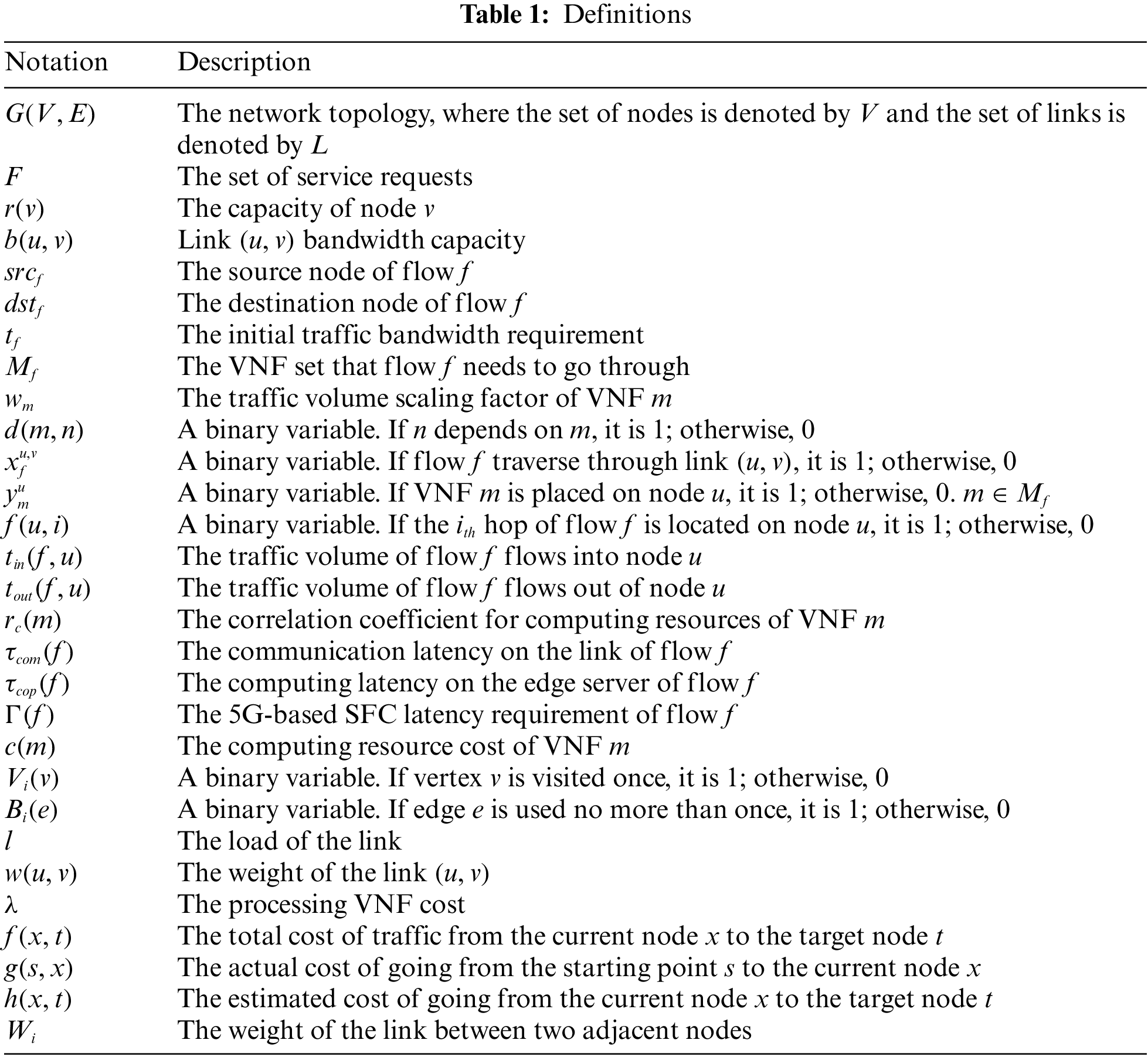
In this section, the studied problem is developed as an ILP model. We provide all the definitions in Table 1.

3.1 Network Model

The input are specifications of the policy and information of the network in our problem. The network is denoted by G = (V, E). The set of links is denoted by E. The set of nodes is denoted by V. Multiple VNFs can be placed on one node, and r(v) represents the node capacity. We use b(u,v) denoting link (u,v)∈E bandwidth capacity. For all arrived service requests, we use F denoting the set of all flows. Considering the characteristics of VNF, (srcf,dstf,tf,Mf) denotes the flow f∈F. srcf denotes the source node of flow f, dstf denotes the destination host, Tf represents the initial bandwidth requirement, and Mf represents the VNF set that flow f needs to go through. We use wm to denote the traffic volume scaling factor of VNF m, and use symbol > to define the dependency relationship between VNFs. For example, m>n denotes that VNF n depends on VNF m, which means the traffic flow of the network has to be processed by VNF m before traverse through VNF n. Note that the VNF dependency has transitivity. It means that if m>n, n>k, then m>k.

3.2 Mathematical Formulation

The model objective is to minimize the total network resource cost. The problem is formulated as an ILP model.

A binary variable d(m,n) is first defined to indicate the dependency between two VNF m and n:

d(m,n)={1m>n0otherwise(1)

Next, a path for the traffic flow f is selected by the controller. A binary variable xfu,v is defined to represent the path passing by:

xfu,v={1flow ftraversethroughlink (u,v)0otherwise(2)

Then, for any traffic flow in the network, the controller deploy its VNFs to the appropriate physical nodes. We use a binary variable ymu to present:

ymu={1VNF m is\ placedonnode u,where m∈Mf0otherwise(3)

We assume flow f passes through a multi-hop path in the network. Different VNFs being placed on the same node are also counted as one hop. If there are N hops in total, we use f(u,i) to indicate the position of the ith hop, where 1≤i≤N:

f(u,i)={1the ithhopofflow fislocatedonnode u0otherwise(4)

In addition, the same node is allowed to deploy multiple VNFs of the same flow to get the optimal solution when the computing resources are sufficient. Therefore, for flow f, there are the following situations:

∃u,i≠j:f(u,i)=f(u,j)=1(5)

Next, we build a mathematical model according to the constraints in the underlying network. In this section, tin(f,u) and tin(f,u) are defined to indicate the traffic volume of flow f flows into and out of node u. For traffic flow f, if the VNF at node u processes it, then the relationship satisfied by tin(f,u) and tout(f,u) is shown as follows:

tout(f,u)=∏m∈Mftin(f,u)⋅wmymu≠0,∀u∈V(6)

Under circumstances that the computing resource cost of VNFs are positively related to the traffic volume, so we give the correlation coefficient rc(m), and use c(m) to indicate the computing resource cost of VNF m:

c(m)=tin(f,u)⋅rc(m)ymu≠0,∀u∈V(7)

The sum of computing resources required must be no more than the node capacity provided by the physical node u. This can be described as:

∑f∈F∑m∈Mfc(m)⋅ymu≤r(u),∀u∈V(8)

In addition, we should guarantee that the coverage of the bandwidth capacity. We present it as follows:

∑f∈FXfu,v⋅tout(f,u)≤b(u,v),∀(u,v)∈E(9)

Since the our VNFs are deployed on the edge servers to get close to the data source, meeting the low latency requirement of 5G, the model must have a latency constraint:

∑(u,v)∈EXfu,vτcom(f)+∑m∈Mfτcop(f)ymu≤Γ(f)(10)

where τcom(f) represents the communication latency on the link, and τcop(f) represents the computing latency on the edge server. Γ(f) represents the 5G-based SFC latency requirement.

To meet the first and last hops of the service request which is at the source node and destination node, respectively, we present following formula:

∑v∈Vxfsrcf,v=1,∑u∈Vxfu,dstf=1,∀f∈F(11)

That each VNF must only be placed on a physical node once is assumed:

∑u∈Vymu=1,∀m∈Mf(12)

For the dependency relationship between VNFs, the following formula gives the constraints that should be satisfied after mapping. It means that for the two virtual network functions of m and n in flow f, if n depends on m, then n will be deployed on the node after m:

(∑i∈[1,N]ynu⋅f(u,i)⋅i−∑i∈[1,N]ymu⋅f(u,i)⋅i)⋅d(m,n)≥0,∀m,n∈Mf(13)

After we map the virtual link of the traffic flow to the physical link, we ensure the law of flow conservation in the network. This can be described as:

∑v∈Vxfu,v−∑v∈Vxfv,u={1if uisthesourcenode−1ifuisthedestinationnode∀r ∈R,∀ v ∈ V0otherwise(14)

In order to quantify computing resources and communication resources in a unified way, we design coefficients α and β to represent the contribution of both resources, where α represents the contribution proportion of computing resources to the objective function, and β represents the contribution proportion of communication resources to the objective function. We first give the contribution formula of total computing resource cost:

Costcop=α∑f∈F∑uc(u)(15)

Then, we give the contribution formula of total communication resource cost:

Costcom=β∑f∈F∑(u,v)∈Exfu,v⋅tout(f,u)(16)

Finally, to minimize the total network resource cost, the ILP model is formulated as follows:

Minimize:Cost=Costcop+Costcom(17)

Subject to: (6)–(15)

3.3 Problem Analysis

By reduction from Hamiltonian Cycle problem, we can prove our problem NP-hard, where the VNFs order constraint is relaxed. Because the Hamiltonian Cycle problem is a classic NP-hard problem, the TAVIP problem is a NP-hard problem. We use the following theorems demonstrating the NP-hardness of the TAVIP problem.

Theorem 1: The TAVIP problem is a NP-hard problem.

Proof: The Hamiltonian Cycle problem is to determine whether there is a simple cycle that passes all vertexes in V, in which repeating nodes shall not exist. As is shown in Fig. 2, consider a Hamiltonian Cycle instance with a directed graph G=(V,E), where the set of vertices is denoted by V and the set of edges is denoted by E. For each vertex v∈V, we have following definition:

Vi(v)={1if visvisitedonlyonce0otherwise(18)

Figure 2: Reduction from hamiltonian cycle to TAPIM

For each edge e∈E we have following definition:

Bi(e)={1if eisusednomorethanonce0otherwise(19)

There shall exist a simple circle that contains each vertex in the graph.

We redefine our optimization problem to a route planning problem. Then we will explain that we can reduce the Hamiltonian Cycle problem to our problem. Consider a TAVIP instance with a graph G′=(V′,E′), where the set of vertices is denoted by V′ and the set of edges is denoted by E′. For each vertex v∈V, two nodes vin, vout assigned with capacity C(vin)=0 and C(vout)=1 are created. The edge (vin,vout)∈E, vin,vout∈V has a bandwidth capacity b(vin,vout)=∞, and for its weight W(vin,vout) we have following definition:

W(vin,vout)={1iftheloadisnomorethanone∞otherwise(20)

We generate a link (uout,vin)∈E′ whose bandwidth capacity is b(uout,vin)=1 and weight is W(uout,vin)=0 for every edge (u,v)∈E. We give a flow f whose source and destination are both the same, Ain, i.e., srcf=dstf=Ain. In G, n is a vertex in V. The initial traffic rate is set to one. Considering a non-ordered VNF set M with V VNFs |M|=|V|, traffic rate changing factor of each VNF m∈M is wm=1.

Definition: We call a function f:δ1→δ2 the mapping reduction from A to B if f

a)   For any β∈δ1, β∈A if f f(β)∈B,

b)   f is a computable function.

Mapping reductions are used to reduce one decision problem to another decision problem. So if we can reduce problem A to problem B in polynomial time, we can transfer the answer of A to the answer of B in polynomial time. By mapping the variable of the Hamiltonian Cycle problem to the variable of our problem, we have

{Vi(v)→W(vin,vout))Bi(e)→b(uout,vin)}(21)

We can reduce the Hamiltonian Cycle problem to our optimization problem through the definition and Eq. (20). In other words, if G has a Hamiltonian Cycle, the TAIVP with G’ and f has a path with minimum cost of |V|. Hence, our optimization problem is NP-hard and an A* algorithm in Section 4 is designed to optimize our problem.

4  Algorithm Design

In this section, a heuristic algorithm called TAIVP is proposed. As is shown in Algorithm 1, the TAIVP algorithm has three main components. For each service request, the algorithm constructs an optimal SFC based on VNF traffic volume scaling factor and dependency by SFC Construction function (line 2). Then, in line 3, it finds a feasible work path with sufficient resources and minimum hops for each SFC by Path Planing function. In line 4, according to the influence of traffic volume scaling factors of VNFs, the SFC is deployed to the determined path by SFC Embedding function [38]. Finally, in line 6, all resource cost in the network is added up by the algorithm.

4.1 SFC Construction

SFC Construction function is used to construct SFC with the lowest network resource cost while satisfying the constraint of the VNF dependency. The most original solution is to put the VNF with smaller traffic volume scaling factor in the front position. Because of the dependency between VNFs, we propose the construction strategy of combining VNFs to minimize network resource cost. We first rank all VNFs in the ascending order of their traffic volume scaling factors. When a VNF has dependency constraint, if its traffic volume scaling factor is smaller than the dependent VNF i in front of it, it must follow i and we combine it with i. Otherwise the restriction has no effect in our design. As is shown in Fig. 3, both sets A and B are combined VNFs.

Figure 3: Placement of VNF sets

We define two parameters w and λ for each VNF, where w represents the traffic volume scaling factor and λ represents the network resource cost of a combined VNF set (a single VNF can be regarded as a VNF set with only one VNF) with the initial bandwidth being 1. Therefore, the definition for a single VNF i is presented as follows:

λi=α⋅rc(i)+β⋅wi(22)

For a combined VNF set with VNF i and VNF j, we have the following definitions:

λ(i,j)=λi+wi⋅λj(23)

w(i,j)=wi⋅wj(24)

To determine the order of two VNF sets without dependency, as shown in Fig. 3, if set A shall be placed in front of set B, then the total cost of such deployment must be less than the total cost of set B in front of set A. We have the following formula:

λA+wA⋅λB≤λB+wB⋅λA⇒(1−wB)/λB≤(1−wA)/λA(25)

This shows that if (1−wA)/λA is regarded as an intrinsic attribute of VNF set A, and VNF with larger value should be placed at the front.

In Algorithm 2, we present the detail of SFC Construction function. The input of the Algorithm 2 is the VNF sets Mf, and the output is the designed SFC. First, we calculate the λi of each VNF and sort them (lines 1–4). Then we select the VNF with highest (1−wi)/λi value (line 6). If the selected VNF has efficient dependency restriction, we combine it with the previous VNF, update their λ and w, and then delete VNFi and VNFj from Mf and add VNFi,j to it (lines 7–12). Otherwise we add VNFi to the end of SFC and delete it from Mf (lines 13–15). Finally, we will get the designed SFC with the lowest netwrok resource cost while satisfying the VNF dependency.

Complexity analysis: We analyze the time complexity of the SFC Construction function. Since the dependency relationship will fix the relative VNFs in order, which makes the SFC construction time shorter, we assume there is no dependency relationship in a service request. The order of any two VNFs can be determined after a round of calculation. The number of VNFs of a service request is denoted by n. The time complexity of sorting (1−wi)/λi is O(nlogn), and the time complexity of sorting VNFs is O(n). So the time complexity of the SFC Construction function is O(nlogn).

4.2 Path Planning

A-star algorithm is a commonly used heuristic search algorithm based on Dijkstra algorithm. It is popular in path planning because of its flexibility, especially in the field of artificial intelligence. It selects the expansion direction of the node reasonably through the evaluation function, and constantly searches for the best path by approaching the destination node. In this way, it can search the node with high probability first, thus improving the search efficiency of the path node.

As shown in Fig. 4, we can see that it leverages an evaluation function to estimate the path cost from the current node to the destination node. The evaluation function is shown as follows:

f(x,t)=g(s,x)+h(x,t)(26)

Figure 4: A-star algorithm schematic

In this formula, x denotes the current node. t denotes the destination node. s denotes the source node. f(x,t) represents the total cost of the path from x to t. g(s,x) represents the actual cost of the path from s to x, which can be obtained by Dijkstra algorithm; h(x,t) represents the estimated cost of the path from x to t, which can be used for the algorithm to search the nodes close to the destination node first. In the process of heuristic search, it is necessary to ensure that h(x,t) is no more than the real cost required from x to t, otherwise the result will be inaccurate, so we set h(x,t) as the shortest path from x to t.

The purpose of path planning is to minimize the resource cost on the work path. Under the condition of SFC construction, the shorter the path, the less the link resource cost. The key point of A-star algorithm is to find g(s,x) from the source node to any accessible adjacent node, estimate the h(x,t) from a adjacent node to the destination node, and calculate the total cost f(x,t). Then the algorithm selects the adjacent node with the lowest total cost and repeat the above operation until we find the shorted path. If the deployment of SFC cannot be completed by the shortest path, A-star algorithm will find a sub-shortest path for the SFC.

As is shown in Algorithm 3, we present the detail of Path Planning function. First, we arrange the service requests according to the initial bandwidth requirement tf in descending order (lines 1, 2). Second, we reverse all edges of the network topology. We take the destination node dstf as the source node, and calculate the shortest path h(x) from dstf to any other node (line 3). Then we create a priority queue Queue to storage nodes with the shortest distance from the node to the source node g(x) and the estimated cost f(x). cnt stores the number of times a node leaving the queue; r record the computing resources that nodes of path can provide (line 4). Next, we put the source node srcf into the queue Queue (line 5). After that it selects the node x with the lowest estimated cost in the queue to determine whether the node is the destination node and the number of times it exits the queue is k. If so, the current path is the k−th shortest path from the source node to the destination node, and the algorithm ends (lines 6–14, 22–24). Otherwise, the algorithm searches the adjacent nodes of node x, and add the information of them to the priority queue (lines 15–21).

4.3 SFC Embedding

Through the processing of the first two functions, we now know the SFC and work path. The problem to be solved in this stage is to ensure the total cost of the whole link is the smallest by deploying VNFs to the determined work path according to the impact of their traffic volume scaling factors on the traffic and its order. A SFC Embedding algorithm is proposed to optimize this problem.

The constructed SFC has K VNFs in sequence with the initial bandwidth being tf. There are N network nodes on the effective work path found by Path Planning algorithm, and the node capacity provided by each node is r(v).

As is shown in Fig. 5, we construct a matrix diagram of N rows and K+1 columns. Each row represents a network node on the work path and each network node can place multiple VNFs. Each column represents a VNF of the SFC arranged in order. The first column represents empty means no VNF is placed. In the figure, the product value below each VNF indicates the total traffic volume scaling factor after the VNF is deployed. The blue dot indicates the VNFs that this node may place. There are K+1 dots in a row, indicating that each node has a opportunity to place any VNF. The line connecting the dots indicates the possible placement from the previous node to the next node. The parameters on the line indicates the weight Wi of the link between two adjacent nodes in this placement case. w multiplied by the initial bandwidth tf is the communication cost on the link. Starting from the first row, we suppose that the computing resource r(v1) of node v1 can meet first two VNFs. Then there are only three possible placement strategies for this node: places 0, 1, or 2 VNFs. The first small dot means that no VNF is placed on node v1, the second small dot means that VNF1 is placed v1, and the third small dot means that v1 has VNF1 and VNF2 placed. Then for the second row, suppose that its computing resource r(v1) of node v2 can meet any two VNFs of VNF1-4. Then we can also places 0, 1, or 2 VNFs on this node. Fig. 5 shows that there are 9 lines between first row and second row, that is, there are 9 possible placement strategies for nodes v1 and v2.

Figure 5: SFC embedding matrix

It can be seen that for each row, the communication cost after the nth VNF is ∏i=1nwi, and so on. After the deployment of the k−th VNF, the communication cost is ∏i=1kwi until it is connected to the last network node vn. When the SFC deployment matrix is complete, what we need to do is to solve the shortest path from the initial dot in the first row to the last dot in the last row. The VNF with w<1 shall be deployed at the front of the link, and the VNF with w>1 shall be deployed at the back of the link. For VNF i and VNF j, if wi>1 but wi+1<1, we will consider them as a VNF set and calculate wi⋅wi+1 to determine their deployment strategy. The location of the dots in this shortest path is our SFC embedding strategy.

As is shown in Algorithm 4, we present the detail of SFC Embedding function. First, we construct a matrix diagram like Fig. 5 (line 1). Then we design all VNF placement strategies without violating restraints (lines 2–11). Finally, we calculate the path and place VNFs to minimize the resource cost under the latency constraint in (lines 12–14).

Complexity analysis: The complexity of time of the SFC Embedding function is analyzed. n denotes the number of nodes and k denotes the number of VNFs. The time complexity of traversing each line to decide whether to keep it or not is O((k−1)(n−1)). The time complexity of calculating w of each VNF or VNF set is O(2k). The time complexity of SFC Embedding is O(n). So the time complexity of the SFC Embedding function is O(kn).

5  Simulation

5.1 Set Up

Our test networks, NSFNET and USNET, are shown in Fig. 6 which are two typical operator networks. NSFNET topology has 14 nodes and 21 links, and USNET topology has 24 nodes and 43 links. We set the capacity of each link to 1000 units and the computing capacity of each node to 100 units. We assume that we would place totally eight types of VNFs in the network. Each traffic volume scaling factor is a random value from 0.01 to 5, and each CPU demand correlation coefficient is a random value from 0.01 to 0.1. As for service requests, we assume the nodes of network entry and export are chosen randomly. We uniformly distribute the initial bandwidth of each SFC in the span of 20 to 80 units. The number of VNFs of each SFC is assumed to be random in the range of 2 to 8. In our study, that how relatively important the computing capacity is denoted by the coefficient α, and that how relatively important the link capacity is denoted by the coefficient β. α is set to 10, and β is set to 1. We uniformly distribute the link latency form 0.01 to 5 ms, and we set the single VNF computing latency 0.5 ms [36,39,40].

Figure 6: Test networks

1)PerformanceMetrics: We use two metrics evaluating the performance of our algorithm: 1) total network resource cost: the total cost of the network resource, which accumulates all service requests. In this paper, we refer to computing resource cost and communication resource cost; 2) request acceptance rate: the percentage of requests deployed with respect to all requests; 3) service response time: the interval from the service request to VNF deployment.

2)Benchmarks: We use the TOSP algorithm in [36] as our main benchmark algorithm. Besides, since there is limited existing solution, we have developed three benchmarks for reference: 1) The sorted VNFs are continuously deployed by the First-fit algorithm on the first physical node with sufficient resources in the path from the beginning; 2) The sorted VNFs are continuously deployed by the Last-fit algorithm on the last physical node with sufficient resources in the path from the end; 3) The sorted VNFs is randomly deployed by the Random-fit algorithm on the work path, and due to its uncertainty, the simulation results are the average values obtained after multiple experiments. These three algorithms need to determine the processing order of VNFs. Their sorting scheme is to multiply the traffic volume scaling factors of each dependency in each traffic flow in turn, and arrange the products in ascending order. In this order, all dependencies can be connected in series to form a chain. Their working paths are all searched one by one through path planning algorithm based on A-star principle.

5.2 Simulation Results

5.2.1 Network Resource Cost with Different Numbers of Service Requests

The results of the network resource cost consumed by the five algorithms under different service requests in NSFNET and USNET network topologies are demonstrated Fig. 7, respectively. In this scenario, the number of VNFs of each service request in NSFNET network is 3 and in USNET network is 4. The initial bandwidth is 40 units, and the K of path planning algorithm is 3. From the figure, we can see that the total network resource cost increases when the number of service requests increases, and the TAIVP algorithm costs the least network resource. On the contrary, the First-fit algorithm has the worst performance. The Last-fit algorithm can achieve a relatively better deployment for the traffic volume scaling factor of each VNF is a random value from 0.01 to 5, and the total traffic volume scaling rate of each traffic flow is the product of their multiplication. As a result, the probability of this value larger than 1 is greater so that when VNFs is deployed from the second half of the path(Last-fit algorithm), the total load is more likely to be less than that from the first half (First-fit algorithm). At the same time, it is obvious that Random-fit algorithm produces results between First-fit algorithm and Last-fit algorithm. The main reason why TOSP algorithm is not as good as TAIVP is that it only considers the minimization of communication resources, and the secondary reason is that it uses the approximate optimal method for SFC construction. Compared with the best of these four benchmark algorithm, TAIVP algorithm saves up to 9.9% and 10.5% network resource cost on average of two topologies for its smarter SFC designing.

Figure 7: Network resource cost and the number of service requests

5.2.2 Network Resource Cost with Different Initial Bandwidth

Fig. 8 shows the impact of the initial bandwidth change of service requests on the network resource cost. The number of VNFs of service requests is the same of the scenario of Fig. 7. The number of service requests is 40, and the K of path planning algorithm is also 3. We can tell that in both NSFNET and USNET topology, the total cost of network resources consumed by the five deployment schemes will increase with the increase of the initial bandwidth, and the cost consumed by the TAIVP algorithm is the least. Compared with the best of these four benchmark algorithm, the TAIVP algorithm reduces the network resource cost by 10.1% and 9.6% on average. This is because the TAIVP algorithm is designed according to the strategy of minimizing the network resource cost in the process of building or deploying the SFC. At the same time, with the increase of the initial bandwidth, the performance advantage of the TAIVP algorithm is more and more obvious.

Figure 8: Network resource cost and initial bandwidth

5.2.3 Network Resource Cost with Different α

In our study, the coefficient of computing resource is denoted by α, and the coefficient of network resource is denoted by β. They represent two critical factors of the total resource cost in the network. Fig. 9 shows Network resource cost vs. α for NSFNET and USNET. The number of VNFs of service requests is the same of the scenario of Fig. 7, and the initial bandwidth is 40 units. The number of service requests is 40, and the K of path planning algorithm is also 3. We can see that when α is smaller (e.g., α = 0 or 5), communication resource cost is more critical than computing resource cost and has lager influence on the total network cost. While when α is larger (e.g., α = 20 or 40), computing resource is more critical than communication resource cost and has lager influence on the total network cost. We can see that with the increase of α, the total network resource cost also shows an increasing trend, and the TAIVP algorithm costs the least network resource. Compared with the best of these four benchmark algorithms, the network resource cost is reduced 11.3% and 10.9% on average by the TAIVP algorithm. At the same time, with the increase of α, the performance advantage of the TAIVP algorithm is more and more obvious.

Figure 9: Network resource cost and α

Beside the cost of network resources, we also need to consider the success rate of traffic flow deployment. Therefore, we will discuss the change of traffic flow acceptance rate of these five algorithms. The traffic flow acceptance rate is that the total number of requests divides the number of successful deployment requests, and the K value of path planning algorithm is set to 3.

5.2.4 Request Acceptance Rate with Different Numbers of Service Requests

The relationship between the traffic flow acceptance rate and the number of service requests is shown in Fig. 10. In the figure, the number of VNF of service requests in NSFNET topology is 3 and in USNET topology is 4, and the initial bandwidth is 40 units. Obviously, when the number of service requests increases, the request acceptance rate in the network is gradually reduced. Simulation results show that the request acceptance rates of TAIVP algorithm are 6.22% and 10.27% higher than the other four algorithms on average of two network topologies. The reason is that the TAIVP algorithm generates the SFC with the lowest resource cost according to the traffic volume scaling factors of VNFs when building the SFC, while the other three algorithms only rank all the dependencies in series. Thus, when the network resources are large enough, TAIVP algorithm can accommodate more service requests. Meanwhile, compared with NSFNET network, the performance advantage of USNET network is more obvious. Especially when the number of service requests increases, the request acceptance rate of TAIVP algorithm decreases more slowly, which shows that TAIVP algorithm is more suitable for large-scale network topology than other three algorithms.

Figure 10: Request acceptance rate and the number of service requests

5.2.5 Request Acceptance Rate with Different Initial Bandwidth

As shown in Fig. 11, different initial bandwidth settings also affect the reception rate of service requests in the network. In the scenario of Fig. 10, the number of VNF remains, and the number of service requests is 40. We can tell that the request receiving rates of TAIVP algorithm in the two topologies are 6.21% and 6.85% higher than those of the other four algorithms on average, which shows that TAIVP algorithm is more suitable for the application scenarios of high-intensity services. So when the initial bandwidth of services is large, the network can effectively deploy more user requests.

Figure 11: Request acceptance rate cost and initial bandwidth

5.2.6 Request Acceptance Rate with Different Numbers of VNFs

In addition, the number of VNFs for service requests also affects the result of the request reception rate. In Fig. 12, the number of service requests in both network topologies is 20, and the initial bandwidth is 40 units. It is not hard to see that when the number of VNF increases, the acceptance rates of TAIVP algorithm are still 8.81% and 7.24% higher on average of two topologies. This is because for First-fit and Last-fit algorithm, their VNF deployment location is relatively centralized, and they do not make good use of the traffic volume scaling factors of VNFs to reduce the network resource cost. And for TOSP algorithm, its sub-optimal SFC constructing strategy can only cover 2 VNFs with dependent relationships. When the VNF number increases, more and more VNFs can be in the same dependency relationship, causing TOSP algorithm no longer valid. Therefore, some links in the network cannot provide enough resources, leading to deployment failure. It can also be seen from the figure that as the deployment of a single traffic flow becomes more complicated, the traffic reception rate is gradually decreasing, especially when the number of VNF in NSFNET network is greater than 4 and in USNET network is greater than 6. This shows that the number of VNFs that USNET network can adapt to is larger for its greater network scale and the planned work path can provide more node resources. Therefore, we can tell that TAIVP algorithm can perform very efficient in large-scale network.

Figure 12: Request acceptance rate cost and the number of VNFs

5.2.7 Service Response Time

As shown in Fig. 13, the service response time is also evaluated. Because NSFNET topology and USNET topology showed similar results, we only demonstrated NSFNET topology here. We first evaluated the service response time under different initial bandwidth. In Fig. 13a, we can see that with the increase of initial bandwidth, the response time of all five algorithms goes up. The First-fit, Last-fit and Random-fit algorithm increase sharply while the TAIVP and TOSP increase slowly. The reason is that when the initial bandwidth increases, the successful acceptance rate of First-fit, Last-fit and Random-fit decreases rapidly. As a result, their response time increases rapidly. The successful acceptance rate of TAIVP and TOSP does not decline so fast, so their response time does not increase so fast. Similarly, from Fig. 13b, we can see that with the increase of the number of VNFs to be deployed, the response time of First-fit, Last-fit and Random-fit rises rapidly, while the response time of TAIVP and TOSP does not rise so rapidly. The reason why TAIVP works better than TOSP is that TAIVP minimizes computing resources and communication resources at the same time, and calculates the most efficient results on SFC construction, while TOSP only considers communication resources, and the construction of SFC is sub-optimal.

Figure 13: Service response time in NSFNET topology

6  Conclusion

In this paper, we jointly optimize SFC design and VNF placement problems to minimize resource cost while taking into account VNF dependency and traffic volume scaling. We first formulated the problem as an ILP model and proved its NP-hardness. Then we proposed and evaluated a heuristic algorithm called TAIVP. Finally, emulation results showed that our algorithm could reduce network cost by 10.2% and increase service request acceptance rate by 7.6% on average. There is a wide range of scenarios where our algorithm can be applied. For example, we can use this algorithm to optimize the positions of VNFs (such as computer vision, natural language processing, intelligent control, etc.) in edge computing-enabled 5G networks. However, there are still some limitations of this paper. First, we didn’t consider the QoS of the service requests, which is an important part in NFV. Besides, the heuristic algorithm can not guarantee the distance of the returned solution to the optimal one. Therefore, in future work, we first plan to modify our ILP model to take account of the QoS of the service requests. Furthermore, we plan to analyze the problem and devise an approximate algorithm with provable approximate solutions.

Funding Statement: This work was supported in part by the Open Research Projects of Zhejiang Lab (No. 2021LC0AB04) and in part by the National Natural Science Foundation of China (NSFC) (Nos. 62171085, 62001087, U20A20156, and 61871097).

Conflicts of Interest: The authors declare that they have no conflicts of interest to report regarding the present study.

References

1. Ning, Z., Dong, P., Wen, M., Wang, X., Guo, L. et al. (2021). 5G-enabled UAV-to-community offloading: Joint trajectory design and task scheduling. IEEE Journal on Selected Areas in Communications, 39(11), 3306–3320. DOI 10.1109/JSAC.2021.3088663. [Google Scholar] [CrossRef]
2. Alsharif, M. H., Hossain, M. S., Jahid, A., Khan, M. A., Choi, B. J. et al. (2022). Milestones of wireless communication networks and technology prospect of next generation (6G). Computers, Materials & Continua, 71(3), 4803–4818. DOI 10.32604/cmc.2022.023500. [Google Scholar] [CrossRef]
3. Hwang, J., Nkenyereye, L., Sung, N., Kim, J., Song, J. (2021). IoT service slicing and task offloading for edge computing. IEEE Internet of Things Journal, 8(14), 11526–11547. DOI 10.1109/JIOT.2021.3052498. [Google Scholar] [CrossRef]
4. Noor, F., Khan, M. A., Al-Zahrani, A., Ullah, I., Al-Dhlan, K. A. (2020). A review on communications perspective of flying ad-hoc networks: Key enabling wireless technologies. applications. Challenges and Open Research Topics, 4(4), 65. [Google Scholar]
5. Goudarzi, M., Wu, H., Palaniswami, M., Buyya, R. (2021). An application placement technique for concurrent IoT applications in edge and fog computing environments. IEEE Transactions on Mobile Computing, 20(4), 1298–1311. DOI 10.1109/TMC.2020.2967041. [Google Scholar] [CrossRef]
6. Wang, X., Ning, Z., Guo, L., Guo, S., Gao, X. et al. (2022). Online learning for distributed computation offloading in wireless powered mobile edge computing networks. IEEE Transactions on Parallel and Distributed Systems, 33(8), 1841–1855. DOI 10.1109/TPDS.2021.3129618. [Google Scholar] [CrossRef]
7. Muhammad, A., Sorkhoh, I., Qu, L., Assi, C. (2021). Delay-sensitive multi-source multicast resource optimization in NFV-enabled networks: A column generation approach. IEEE Transactions on Network and Service Management, 18(1), 286–300. DOI 10.1109/TNSM.2021.3049718. [Google Scholar] [CrossRef]
8. Wang, M., Cheng, B., Li, B., Chen, J. (2019). Service function chain composition and mapping in NFV-enabled networks. IEEE World Congress on Services, 2642, 331–334. DOI 10.1109/SERVICES.2019.00092. [Google Scholar] [CrossRef]
9. Ning, Z., Yang, Y., Wang, X., Guo, L., Gao, X. et al. (2021). Dynamic computation offloading and server deployment for UAV-enabled multi-access edge computing. IEEE Transactions on Mobile Computing. DOI 10.1109/TMC.2021.3129785. [Google Scholar] [CrossRef]
10. Sun, G., Zhou, R., Sun, J., Yu, H., Vasilakos, A. V. (2020). Energy-efficient provisioning for service function chains to support delay-sensitive applications in network function virtualization. IEEE Internet of Things Journal, 7(7), 6116–6131. DOI 10.1109/JIoT.6488907. [Google Scholar] [CrossRef]
11. Dong, L., da Fonseca, N. L. S., Zhu, Z. (2020). Application-driven provisioning of service function chains over heterogeneous NFV platforms. IEEE Transactions on Network and Service Management, 18(3), 3037–3048. DOI 10.1109/TNSM.2020.3035254. [Google Scholar] [CrossRef]
12. Fan, J., Guan, C., Zhao, Y., Qiao, C. (2017). Availability-aware mapping of service function chains. IEEE Conference on Computer Communications, Atlanta, GA, USA. [Google Scholar]
13. Ghaznavi, M., Shahriar, N., Kamali, S., Ahmed, R., Boutaba, R. (2017). Distributed service function chaining. IEEE Journal on Selected Areas in Communications, 35(11), 2479–2489. DOI 10.1109/JSAC.2017.2760178. [Google Scholar] [CrossRef]
14. Shah, H. A., Zhao, L. (2020). Multiagent deep-reinforcement-learning-based virtual resource allocation through network function virtualization in Internet of Things. IEEE Internet of Things Journal, 8(5), 3410–3421. DOI 10.1109/JIoT.6488907. [Google Scholar] [CrossRef]
15. Ye, Z., Cao, X., Wang, J., Yu, H., Qiao, C. (2016). Joint topology design and mapping of service function chains for efficient, scalable, and reliable network functions virtualization. IEEE Network, 30(3), 81–87. DOI 10.1109/MNET.2016.7474348. [Google Scholar] [CrossRef]
16. Wang, X., Ning, Z., Guo, S., Wen, M., Poor, V. (2021). Minimizing the age-of-critical-information: An imitation learning-based scheduling approach under partial observations. IEEE Transactions on Mobile Computing. DOI 10.1109/TMC.2021.3053136. [Google Scholar] [CrossRef]
17. Herrera, J. G., Botero, J. F. (2016). Resource allocation in NFV: A comprehensive survey. IEEE Transactions on Network and Service Management, 13(3), 518–532. DOI 10.1109/TNSM.2016.2598420. [Google Scholar] [CrossRef]
18. Ma, W., Medina, C., Pan, D. (2015). Traffic-aware placement of NFV middleboxes. 2015 IEEE Global Communications Conference (GLOBECOM), San Diego, CA, USA. [Google Scholar]
19. Citrix, CloudBridge (2017). https://www.citrix.com/content/dam/citrix/enus/documents/products-solutions/cloudbridge-technical-overview.pdf. [Google Scholar]
20. Miller, M. J., Vucetic, B., Berry, L. (1993). Satellite communications: Mobile and fixed services. Berlin, Germany: Springer Science & Business Media. [Google Scholar]
21. https://www.barracuda.com/assets/docs/Datasheets/Barracuda. [Google Scholar]
22. Jalalitabar, M., Luo, G., Kong, C., Cao, X. (2016). Service function graph design and mapping for NFV with priority dependence. 2016 IEEE Global Communications Conference (GLOBECOM), Washington DC, USA. [Google Scholar]
23. Wang, X., Ning, Z., Guo, S., Wen, M., Guo, L. et al. (2021). Dynamic UAV deployment for differentiated services: A multi-agent imitation learning based approach. IEEE Transactions on Mobile Computing. DOI 10.1109/TMC.2021.3116236. [Google Scholar] [CrossRef]
24. Ghai, K. S., Choudhury, S., Yassine, A. (2020). Efficient algorithms to minimize the end-to-end latency of edge network function virtualization. Journal of Ambient Intelligence and Humanized Computing, 11(10), 3963–3974. DOI 10.1007/s12652-019-01630-6. [Google Scholar] [CrossRef]
25. Kuo, J. J., Shen, S. H., Kang, H. Y., Yang, D. N., Tsai, M. J. et al. (2017). Service chain embedding with maximum flow in software defined network and application to the next-generation cellular network architecture. IEEE Conference on Computer Communications, Atlanta, GA, USA. [Google Scholar]
26. Pham, T. M., Fdida, S., Binh, H. T. T. (2017). Online load balancing for network functions virtualization. 2017 IEEE International Conference on Communications (ICC), Paris, France. [Google Scholar]
27. Li, Y., Phan, L. T. X., Loo, B. T. (2016). Network functions virtualization with soft real-time guarantees. 35th Annual IEEE International Conference on Computer Communications, San Francisco, CA, USA. [Google Scholar]
28. Sallam, G., Gupta, G. R., Li, B., Ji, B. (2018). Shortest path and maximum flow problems under service function chaining constraints. IEEE Conference on Computer Communications, Honolulu, HI, USA. [Google Scholar]
29. Fei, X., Liu, F., Xu, H., Jin, H. (2018). Adaptive VNF scaling and flow routing with proactive demand prediction. IEEE Conference on Computer Communications, Honolulu, HI, USA. [Google Scholar]
30. Pham, C., Tran, N. H., Ren, S., Saad, W., Hong, C. S. (2017). Traffic-aware and energy-efficient VNF placement for service chaining: Joint sampling and matching approach. IEEE Transactions on Services Computing, 13(1), 172–185. DOI 10.1109/TSC.4629386. [Google Scholar] [CrossRef]
31. Yu, R., Xue, G., Zhang, X. (2017). QoS-aware and reliable traffic steering for service function chaining in mobile networks. IEEE Journal on Selected Areas in Communications, 35(11), 2522–2531. DOI 10.1109/JSAC.2017.2760158. [Google Scholar] [CrossRef]
32. Ning, Z., Sun, S., Wang, X., Guo, L., Guo, S. et al. (2021). Blockchain-enabled intelligent transportation systems: A distributed crowdsensing framework. IEEE Transactions on Mobile Computing. DOI 10.1109/TMC.2021.3079984. [Google Scholar] [CrossRef]
33. Lin, T., Zhou, Z., Tornatore, M., Mukherjee, B. (2016). Demand-aware network function placement. Journal of Lightwave Technology, 34(11), 2590–2600. DOI 10.1109/JLT.2016.2535401. [Google Scholar] [CrossRef]
34. Huang, H., Guo, S., Wu, J., Li, J. (2016). Joint middlebox selection and routing for software-defined networking. 2016 IEEE International Conference on Communications (ICC), Kuala Lumpur, Malaysia. [Google Scholar]
35. Jalalitabar, M., Guler, E., Zheng, D., Luo, G., Tian, L. et al. (2018). Embedding dependence-aware service function chains. Journal of Optical Communications and Networking, 10(8), C64–C74. DOI 10.1364/JOCN.10.000C64. [Google Scholar] [CrossRef]
36. Ma, W., Sandoval, O., Beltran, J., Pan, D., Pissinou, N. (2017). Traffic aware placement of interdependent NFV middleboxes. IEEE Conference on Computer Communications, Atlanta, GA, USA. [Google Scholar]
37. Siasi, N., Jasim, M. A., Crichigno, J., Ghani, N. (2019). Container-based service function chain mapping. 2019 Southeast Conference, Huntsville, AL, USA. [Google Scholar]
38. Fu, X., Yu, F. R., Wang, J., Qi, Q., Liao, J. (2019). Dynamic service function chain embedding for NFV-enabled IoT: A deep reinforcement learning approach. IEEE Transactions on Wireless Communications, 19(1), 507–519. DOI 10.1109/TWC.7693. [Google Scholar] [CrossRef]
39. Alliance, N. G. M. N. (2015). 5G white paper. In: Next generation mobile networks. Frankfurt, Germany: NGMN. [Google Scholar]
40. Laghrissi, A., Taleb, T., Bagaa, M., Flinck, H. (2017). Towards edge slicing: VNF placement algorithms for a dynamic & realistic edge cloud environment. 2017 IEEE Global Communications Conference, Singapore. [Google Scholar]
Cite This Article
Copyright © 2023 The Author(s). Published by Tech Science Press.
This work is licensed under a Creative Commons Attribution 4.0 International License , which permits unrestricted use, distribution, and reproduction in any medium, provided the original work is properly cited.
Downloads
Citation Tools