Peridynamic Shell Model Based on Micro-Beam Bond

1  Introduction

Peridynamic (PD) theory was proposed by Silling [1] as a new formulation of the classical continuum mechanics (CCM) to solve fracture and failure issues. The PD equations of motion appear as integral-differential equations [2], and the integral does not depend on the continuity of the displacement. Thus, PD theory is spontaneously applied to analyze and solve discontinuity problems, such as crack propagation. In recent years, PD theory has been rapidly developed and applied to fracture or damage analysis of solid structures, such as the fracture problems of isotropic and anisotropic materials [3–5], the problems of plasticity [6–8], the crack branch [9–11] and impact [12] of brittle materials, composite materials [13–15], crack bending problem [16], and nonlinear analysis [17,18].

However, the calculation efficiency of PD models is usually lower than that of other traditional numerical methods, such as the finite element method (FEM), especially for complex structures. The coupling method is a strategy to improve calculation efficiency. Han et al. [19] proposed a local/non-local coupling model via the Arlequin approach; this model couples energy equations of the PD and CCM models in an overlapping domain. Han et al. [20] presented a hybrid adaptive local-continuum damage/PD model by using the morphing method [21,22]. Structural idealization is often employed in engineering as a useful method to reduce the calculation time of PD models. Silling et al. [23] proposed a two-dimensional (2D) PD model for membranes and used this model for the numerical simulation of membrane stretching and dynamic tearing. Gerstle et al. [24] proposed the micropolar PD model that has two stiffness parameters. This model is mainly used to solve 2D plane problems. O’Grady et al. [25] introduced a non-ordinary state-based PD (SBPD) Kirchhoff-Love plate model based on beam models to represent the bending deformation of the plate, which is derived from the concept of a rotating spring with the bond between two material points. Taylor et al. [26] presented a 2D bond-based PD (BBPD) plate model through the asymptotic analysis of thin plates. This model can effectively analyze thin plate structures, including fractures caused by bending. Diyaroglu et al. [27] proposed a new PD Mindlin plate model based on the BBPD formulation while accounting for transverse shear deformation. The PD equations of motion were established and simplified to the same form as those of the classical Mindlin plate equations. Chowdhury et al. [28] proposed an SBPD model for linear elastic shells by introducing a shear correction factor and a shear deformation correction considering shell thickness. Taştan et al. [29] developed a PD model for orthotropic Kirchhoff thin plates based on the BBPD formulation by using the homogenized approach. Sarego et al. [30] proposed a 2D linearized ordinary SBPD model for elastic deformation and computed the stiffness matrix for 2D plane stress/strain conditions, which is suitable for constructing membrane structures. Yang et al. [31] implemented the PD Mindlin plate formulations presented by Diyaroglu et al. [27] in the FEM framework. Nguyen et al. [32] developed a new ordinary SBPD model to predict the thermomechanical behaviors of 3D shell structures with six degrees of freedom, providing numerical methods and computational steps to deal with complex shell structures. Yang et al. [33] proposed a new PD Kirchhoff plate model based on the SBPD formulation, which is computationally efficient because each material point of the plate model has only one degree of freedom. Yolum et al. [34] presented a PD formulation for orthotropic Mindlin plates with transverse shear deformation. Vazic et al. [35] established a PD model for Mindlin plates based on Winkler’s elastic theory, which is an extension of the Mindlin plate model proposed by Diyaroglu et al. [27]. Oterkus et al. [36] developed a new PD formulation for shell membranes. PD equations of motion were established by using Euler-Lagrange equations, and the bond constant of the shell membrane was determined by comparing PD equations of motion with classical equations of motion under a special condition that horizon tends to zero. Zhang et al. [37] developed a SBPD theory for nonlinear Reissener-Mindlin shells to model and predict large deformations of thick-walled shell structures. The controlling equations of the SBPD shell theory were derived by the non-local balance laws and the kinematic assumptions of Reissner and Mindlin plate and shell theories. Yang et al. [38] proposed a new SBPD model for functionally graded Kirchhoff plates and obtained the equations of motion of the proposed model by using the Euler-Lagrange equations and Taylor expansion. Zhang et al. [39] developed a non-local stress resultant-based geometrically-exact shell theory, which can simulate fracture and crack extension in shell structures under finite deformations. Shen et al. [40,41] proposed a PD shell model based on the micro-beam bond via the interpolation method, which is the foundation of this study.

The structural idealization strategies for PD plate and shell models proposed above can be divided into two types: BBPD model and SBPD model. Compared with the SBPD model, the BBPD model has the advantages of easy programming, simple calculation, and high calculation efficiency and has a wide range of application prospects. In the study, the in-plane deformation part of the PD shell in our previous work [40] is improved, and a new fracture criterion based on the strain energy density (SED) of the micro-beam bond is proposed. The reconstruction process of the whole PD shell model is described in detail through the strain homogenization method. First, the deformations of each endpoint of the micro-beam bond are calculated by the interpolation method. Second, the micro-potential energy of the axial, torsional, and bending deformations of the bond can be established from the deformations of endpoints. Finally, the micro moduli of the shell model can be obtained via the equivalence principle of SED.

The rest of this paper is organized as follows. Section 2 reviews the basic formulations of the micro-beam bond with axial, torsional, and bending deformations. Section 3 mainly describes the derivation process of the micro moduli of various deformations in the PD shell model and presents a new energy failure criterion of the micro-beam bond for PD shells. In Section 4, some numerical examples are given, including a V-shaped notch plate under pressure loading, a notched plate under stretching, a notched cylinder under internal pressure, and a notched S-shaped curved shell under stretching. Finally, Section 5 provides the conclusions.

2  Micro-Beam Bond

As shown in Fig. 1, the micro-beam bond is assumed to be composed of point xi and its adjacent point xj, which is located in the neighborhood horizon Hxi. The neighborhood horizon of point xi is a circle of radius δ centered on it. For the local coordinate system of the neighborhood horizon Hxi, the normal of the horizon is defined as the Z-axis, and the X-axis and the Y-axis lie in the plane of the horizon and are orthogonal, respectively. For the local coordinate system of the micro-beam bond, the x-axis is defined as the vector from point xi to point xj, the z-axis is in the same direction as the Z-axis, and the y-axis is perpendicular to the x-axis. Each micro-beam bond is subjected not only to axial deformation but also to torsional and bending deformations. The micro moduli of various deformations for the micro-beam bond model can be solved independently.

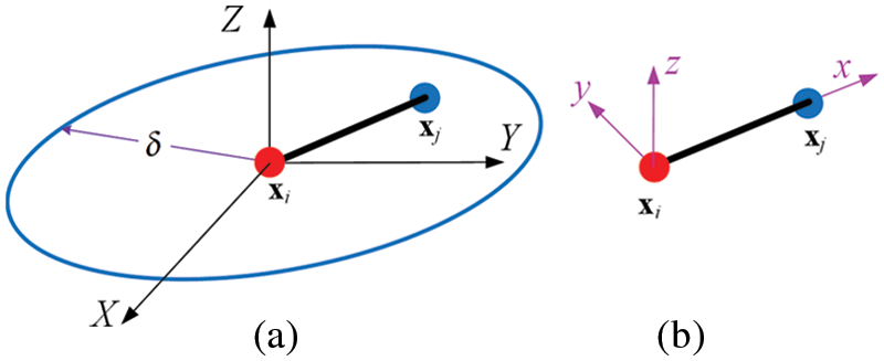
Figure 1: Micro-beam bond with its (a) horizon and (b) local coordinate system

In the local coordinate system of the micro-beam bond, the relationship between the force/moment densities and displacements of endpoints of the micro-beam bond can be expressed as

F=Ku

where

F={fixfiyfizmixmiymizfjxfjyfjzmjxmjymjz}Tu={uiviwiθixθiyθizujvjwjθjxθjyθjz}TK=∫01BTDPDBξdχ(1)

in which B and DPD can be expressed as follows

B=[−1ξ000001ξ000000012χ−6ξ20−6χ−4ξ000−12χ−6ξ20−6χ−2ξ0012χ−6ξ20006χ−4ξ0−12χ−6ξ20006χ−2ξ000−1ξ000001ξ00](2)

and

DPD=[caxcbycbzctor](3)

In Eqs. (1)–(3), χ is the shape parameter whose value ranges from 0 to 1; ξ is the length of the micro-beam bond; and cax, cby, cbz, and ctor are the axial deformation parameter, the bending deformation parameter around the y-axis, the bending deformation parameter around the z-axis, and the torsional deformation parameter, respectively.

3  PD Shell Model

As shown in Fig. 2, the horizon Hxi of point xi is assumed to be exactly enclosed by a square element with nodes 1, 2, 3, and 4, and the length of the square element is L=2δ. For the local coordinate system XYZ of the square element, the X-axis is defined as the vector from node 1 to node 2, the Y-axis is the vector from node 2 to node 3, which is perpendicular to the X-axis, and the Z-axis is the normal of the square element. For the convenience of calculation, the homogenization assumption for the region within the neighborhood horizon of point xi can be extended to any region within the square element, considering that the overlapping region between the neighborhood horizon of point xi and the square element occupies the majority of the square element.

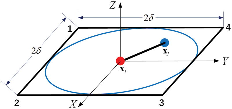
Figure 2: Horizon of point xi is exactly enclosed by a square element

3.1 Micro Moduli of in-Plane Deformation for PD Shells

The in-plane deformation only includes the translational displacement of the X-axis and the Y-axis and the rotation angle displacement around the Z-axis. Therefore, in the coordinate system of the square element, the translational displacement along the X-axis and the Y-axis and the rotation angle around the Z-axis of each node can be defined as UI, VI, and ΘIZ, respectively. The in-plane displacement vector of the square element can be expressed as

U¯e={U¯1TU¯2TU¯3TU¯4T}T(4)

where

U¯IT={UIVIΘIZ}(I=1,2,3,4)

The in-plane displacement vector at any position in the square element can be expressed by the Allman interpolation function [42] and Eq. (4) as

U¯(p,q)={UVΘZ}T=N¯(p,q)U¯e(5)

where N¯(p,q) is the interpolation function, as described in Appendix A.

According to Eq. (5), the in-plane displacement vector at endpoints xi and xj of the micro-beam bond in the local coordinate system XYZ can be obtained as

U¯={UiViΘiZUjVjΘjZ}T=R¯U¯e

where R¯ is the interpolation matrix, specifically

R¯=[N¯(pi,qi)N¯(pj,qj)]

In the local coordinate system of the micro-beam bond, the in-plane displacement vector at endpoints xi and xj of the micro-beam bond is defined as

u¯={uiviθizujvjθjz}T

Through coordinate transformation, the in-plane displacement vector at endpoints xi and xj of the micro-beam bond in its local coordinate system can be obtained as

u¯=T¯U¯=T¯R¯U¯e(6)

where T¯ is the coordinate transformation matrix of the two local coordinate systems of the square element and the micro-beam bond. Assuming that the Z-axis and the z-axis of the two local coordinate systems coincide, we obtain

T¯=[cos⁡θsin⁡θ0000−sin⁡θcos⁡θ0000001000000cos⁡θsin⁡θ0000−sin⁡θcos⁡θ0000001]

where θ is the angle between the x-axis and the X-axis.

As shown in Fig. 3, the micro-beam bond can only be subjected to axial deformation along the x-axis and transversal deformation around the z-axis for the in-plane deformation. Thus, the strain of the micro-beam bond can be expressed in the local coordinate system of the micro-beam bond as

ε¯=[εxκz]T=B¯u¯(7)

where εx, κz represent the axial strain and the curvature in the z-axis direction, respectively, and

B¯=[−1ξ001ξ00012χ−6ξ26χ−4ξ0−12χ−6ξ26χ−2ξ]

where χ is the shape parameter, and ξ is the length of the bond.

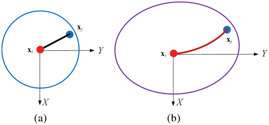
Figure 3: Micro-beam bond subjected to axial and transversal deformation for the in-plane deformation (a) undeformed state and (b) deformed state

Substituting Eq. (6) into Eq. (7) can be obtained as

ε¯=B¯T¯R¯U¯e(8)

According to the homogenization assumption, the strain in the square element is assumed to be equal everywhere and is ε¯XY=[εXεYγXY]T. Thus, the in-plane displacement vector of the square element can be defined as

U¯e=[−εXδ−γXYδ−εYδ−γXY2εXδ−γXYδ−εYδ−γXY2εXδ+γXYδεYδ−γXY2−εXδ+γXYδεYδ−γXY2]T(9)

where εX, εY, and γXY represent the positive strain in the X-axis direction, the positive strain in the Y-axis direction, and the shear strain in the X-axis and the Y-axis directions, respectively.

Substituting Eq. (9) into Eq. (8) can be obtained as

ε¯=[εXcos2θ+εYsin2θ+γXYsin⁡θcos⁡θ6(2χ−1)[(εX−εY)cos⁡θsin⁡θ−γXY(cos2θ−12)]ξ]=T¯ξε¯XY(10)

where

T¯ξ=[cos2θsin2θsin⁡θcos⁡θ6(2χ−1)sin⁡θcos⁡θξ−6(2χ−1)sin⁡θcos⁡θξ−6(2χ−1)(cos2θ−12)ξ]

The micro moduli matrix of the micro-beam bond corresponding to axial and transversal deformations is defined as

D¯PD=[caxcbz](11)

Therefore, the micro-potential energy of the micro-beam bond can be expressed by Eqs. (10) and (11) as

ω¯=12∫xixjε¯TD¯PDε¯dx=12∫01ε¯TD¯PDε¯ξdχ=12∫01ε¯XYTT¯ξTD¯PDT¯ξε¯XYξdχ(12)

Then, the in-plane SED of point xi in PD theory can be expressed by Eq. (12) as

W¯PD(xi)=t∫0δ∫02π12ω¯ξdθdξ=ε¯XYT(t4∫0δ∫02π∫01T¯ξTD¯PDT¯ξξ2dχdθdξ)ε¯XY(13)

where the factory 12 represents that each endpoint of the bond owns only half of the energy in the micro-beam bond, and t is the thickness of the square element.

The in-plane SED of point xi in CCM can be expressed as

W¯CCM(xi)=12ε¯XYTDmε¯XY(14)

where

Dm=E1−ν2[1ν0ν10001−ν2]

where E is Young’s modulus, and ν is Poisson’s ratio.

By setting Eq. (13) equal to Eq. (14), the values of cax and cbz can be obtained as

cax=6Eπtδ3(1−ν),cbz=E(1−3ν)6πtδ(1−ν2)(15)

3.2 Micro Moduli of Bending Deformation for PD Shells

The bending deformation only includes the transversal displacement along the Z-axis and the rotational displacement around the X-axis and the Y-axis. Therefore, in the coordinate system of the square element, the transversal displacement along the Z-axis and the rotation angles around the X-axis and the Y-axis of each node can be defined as WI, ΘIX, and ΘIY, respectively. The bending displacement vector of the square element can be expressed as

U~e={U~1TU~2TU~3TU~4T}T(16)

where

U~IT={WIΘIXΘIY}(I=1,2,3,4)

The bending displacement vector at any position of the square element can be expressed by a cubic interpolation function [40] and Eq. (16) as

U~(p,q)={WΘXΘY}T=N~(p,q)U~e(17)

where N~(p,q) is the interpolation function, as described in Appendix B.

According to Eq. (17), the bending displacement vector at endpoints xi and xj of the micro-beam bond in the local coordinate system XYZ can be obtained as

U~={WiΘiXΘiYWjΘjXΘjY}T=R~U~e

where R~ is the interpolation matrix, specifically

R~=[N~(pi,qi)N~(pj,qj)]

In the local coordinate system of the micro-beam bond, the bending displacement vector at endpoints xi and xj of the micro-beam bond is defined as

u~={wiθixθiywjθjxθjy}T

Through coordinate transformation, the bending displacement vector at endpoints xi and xj of the micro-beam bond in its local coordinate system can be obtained as

u~=T~U~=T~R~U~e(18)

where T~ is the coordinate transformation matrix of the two local coordinate systems of the square element and the micro-beam bond. Assuming that the Z-axis and the z-axis of the two local coordinate systems coincide, we obtain

T~=[1000000cos⁡θsin⁡θ0000−sin⁡θcos⁡θ0000001000000cos⁡θsin⁡θ0000−sin⁡θcos⁡θ]

As shown in Fig. 4, the micro-beam bond can only be subjected to transversal deformation around the y-axis and torsional deformation around the x-axis. Thus, the strain of the micro-beam bond can be expressed in the local coordinate system of the micro-beam bond as

ε~=[κyϕx]T=B~u~(19)

where κy, ϕx represent the curvature in the y-axis direction and the torsional curvature, respectively, and

B~=[12χ−6ξ20−6χ−4ξ−12χ−6ξ20−6χ−2ξ0−1ξ001ξ0]

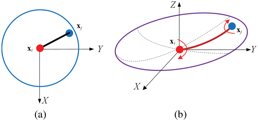
Figure 4: Micro-beam bond subjected to transversal and torsional deformation for the bending deformation (a) undeformed state and (b) deformed state

Substituting Eq. (18) into Eq. (19) can be obtained as

ε~=B~T~R~U~e(20)

According to the homogenization assumption, the strain in the square element is assumed to be equal everywhere and is ε~XY=[κYκXκXY]T. Thus, the bending displacement vector of the square element can be defined as

U~e=[κXYδ22(−κX−κXY2)δ(κY+κXY2)δ−κXYδ22(−κX+κXY2)δ(−κY+κXY2)δκXYδ22(κX+κXY2)δ(−κY−κXY2)δ−κXYδ22(κX−κXY2)δ(κY−κXY2)δ]T(21)

where κX, κY, and κXY represent the curvature in the X-axis direction, the curvature in the Y-axis direction, and the torsional curvature in the X-axis and the Y-axis directions, respectively.

Substituting Eq. (21) into Eq. (20) can be obtained as

ε~=[κYcos2θ+κXsin2θ+κXYsin⁡θcos⁡θ(κX−κY)sin⁡θcos⁡θ+(cos2θ−12)κXY]=T~ξε~XY(22)

where

T~ξ=[cos2θsin2θsin⁡θcos⁡θ−sin⁡θcos⁡θsin⁡θcos⁡θcos2θ−12]

The micro moduli matrix of the micro-beam bond corresponding to bending and torsional deformations is defined as

D~PD=[cbyctor](23)

Therefore, the micro-potential energy of the micro-beam bond can be expressed by Eqs. (22) and (23) as

ω~=12∫xixjε~TD~PDε~dx=12∫01ε~TD~PDε~ξdχ=12∫01ε~XYTT~ξTD~PDT~ξε~XYξdχ(24)

Then, the bending SED of point xi in PD theory can be expressed by Eq. (24) as

W~PD(xi)=t∫0δ∫02π12ω~ξdθdξ=ε~XYT(t4∫0δ∫02π∫01T~ξTD~PDT~ξξ2dχdθdξ)ε~XY(25)

The bending SED of point xi in CCM can be expressed as

W~CCM(xi)=12tε~XYTDbε~XY(26)

where

Db=Et312(1−ν2)[1ν0ν10001−ν2]

By setting Eq. (25) equal to Eq. (26), the values of cby and ctor can be obtained as

cby=Et2πδ3(1−ν),ctor=Et(1−3ν)2πδ3(1−ν2)(27)

So far, the four micro moduli of various deformations for the PD shell model in Eqs. (15) and (27) have all been solved, and the stiffness matrix of a micro-beam bond for PD shells can be formed easily.

3.3 Failure Criterion

By comparing the relationship between the elongation rate s and the critical elongation rate s0 of the bond between two material points, this single judgment criterion cannot accurately describe the damage degree of the micro-beam bond. In this study, the fracture criterion based on the idea of strain energy is adopted to simulate the cracks. The proposed PD shell model belongs to the 2D condition. As shown in Fig. 5, similar to the 3D condition, the fracture energy [43,44], i.e., the energy required to open a new fracture surface per unit area, can be determined by the energy released by breaking all bonds across the unit fracture surface. Assuming that the critical micro-potential energy of each bond is ωc, the integral equation of the fracture energy Gc for the 2D condition can be defined as

Gc=2t∫0δ∫zδ∫0cos−1z/ξωcξdφdξdz(28)

where t is the thickness of the shell and ωc can be expressed as

ωc=12∫xixjεTDPDεdx(29)

where

ε=[εxκyκzϕx]T

where εx, κy, κz, and ϕx represent the axial strain, the curvature in the y-axis and the z-axis directions and the torsional curvature of the micro-beam bond, respectively.

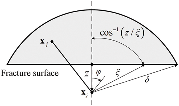
Figure 5: Schematic of the fracture surface

Assuming that the micro-beam bond is uniformly deformed in the neighborhood horizon of point xi, all strains in the neighborhood horizon are equal. Therefore, Eq. (29) can be rewritten as

ωc=12εTDPDεξ(30)

where ξ is the length of the micro-beam bond.

Then, substituting Eq. (30) into Eq. (28), the integral fracture energy equation can be calculated as

Gc=2t∫0δ∫zδ∫0cos−1z/ξωcξdφdξdz=tδ42(12εTDPDε)(31)

Finally, the energy failure criterion of a micro-beam bond can be expressed by Eq. (31) as

ω¯bond=12εTDPDε=2Gctδ4

4  Numerical Examples

4.1 V-Shaped Notch Plate under Pressure Loading

A soda-lime brittle glass plate is selected to demonstrate that the proposed shell model can simulate its crack propagation. The geometry and dimensions of the glass specimen are shown in Fig. 6. Thec sample has the dimension of width W=100mm, height H=150mm, and thickness t=4.65mm. There is a V-shaped notch with an angle of 40∘ on the left side of the sample, and a pre-crack exists at the end of the V-shaped notch. The material properties of the specimen are taken from the literature [45], with Young’s modulus of E=72GPa, Poisson’s ratio of ν=0.23, density of ρ=2440kg/m3, and fracture energy of Gc=3.8J/m2. In the experiment [46], the impact effect on the V-shaped notch is caused by an impactor. Instead of simulating the impactor itself, the notch pressure load is chosen to be estimated in the computational tests to reduce the computational cost of the model. The loading conditions for the notch pressure load are taken from the literature [45], where it is assumed that the load is uniformly distributed along the loading area. Only one layer of material points of the V-shaped notch plate is discretized, with a discretization spacing of Δ=0.5mm. According to suggestions of the literature [47], the selected neighborhood horizon of the material points is δ=3Δ, and the time increment step is Δt=1×10−7 s, which is sufficient to satisfy the stability condition of numerical integration. In this study, a precise volume correction algorithm [48] for 2D PD models is introduced to improve the computational accuracy of numerical integration.

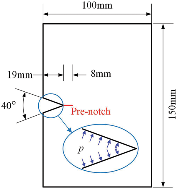
Figure 6: Geometry and dimensions of the V-shaped notch plate

Numerical results are shown in Figs. 7a–7c. As the loading time is prolonged, the crack propagates slowly in the pre-crack direction and the crack bifurcation appears at approximately 60 μs, at a position 60mm away from the left side of the sample, with a bifurcation angle of around 45∘. Two bifurcated crack propagation paths can be observed at the front end of the plate. Experimental results provided in [46] are shown in Fig. 7d. Numerical results in Fig. 7c are in good agreement with experimental results of fractured specimens in Fig. 7d, which shows that the PD shell model and fracture criterion proposed in this study can simulate the crack propagation path very accurately.

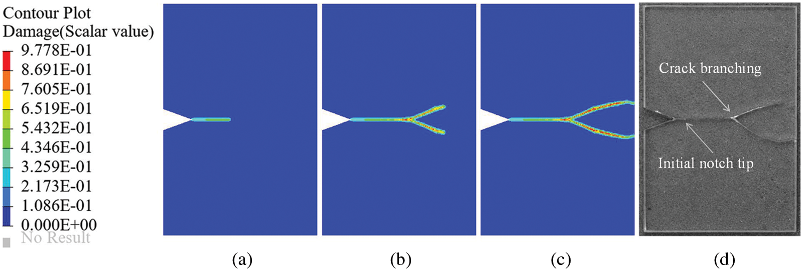
Figure 7: Numerical results of crack propagation for the V-shaped notch plate at loading time of (a) 45 μs, (b) 81 μs, and (c) 112 μs; (d) experimental photographs of fractured specimens, reproduced with the permission of [46], copyright @ Journal of the Mechanics and Physics of Solids, 2018

4.2 Pre-Notched Plate under Stretching

As shown in Fig. 8, the material characteristics, geometric shape, and boundary conditions of the rectangular thin plate are selected as described in literature [49]. The rectangular thin plate has the dimension of length L=100mm, width W=40mm, and thickness t=1mm. The pre-notch is located in the middle of the left side of the rectangular thin plate, whose length is l=50mm. The Young’s modulus, density, Poisson’s ratio, and fracture energy of the thin plate are E=72GPa, ρ=2440kg/m3, ν=1/3, and Gc=135J/m2, respectively. The tensile loading with equal magnitude and the opposite direction is exerted to the upper and lower edges of the thin plate, whose magnitude is kept constant as σ=12MPa throughout the simulation. The neighborhood horizon of the material point is δ=3Δ, and the same fracture criterion as in the previous example is selected.

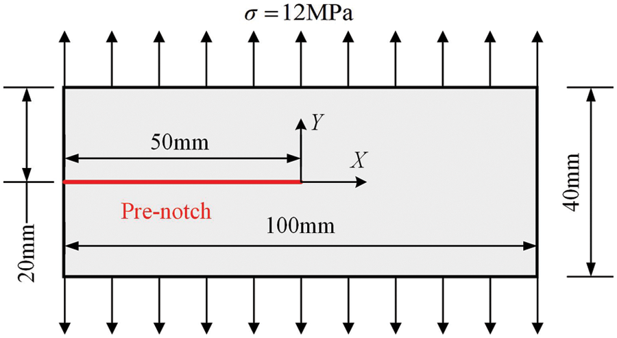
Figure 8: Dimensions and boundary conditions of the pre-notched plate

Four discrete mesh sizes of 1.25, 1, 0.8, and 0.5 mm are selected to investigate the effect of mesh refinement on cracks, respectively. The crack propagation paths of the plate using four uniform grids at 47 μs are shown in Fig. 9. The tensile loading on the upper and lower edges of the thin plate increases abruptly and then remains constant after reaching the required value. As the loading time is prolonged, the crack propagation path slowly expands along the direction (X-axis) of the pre-crack until near 21 μs, crack bifurcation occurs, and two bifurcated crack propagation paths can be observed at the front end of the plate. The crack propagation paths are highly similar for all four models. As the horizon decreases, the damage region becomes smaller, i.e., the damage region becomes more precise. The fine mesh captures the degree of damage more accurately than the coarse mesh. Numerical results show that the crack propagation paths predicted by the proposed PD shell model are roughly similar to the numerical results in the references [48,49].

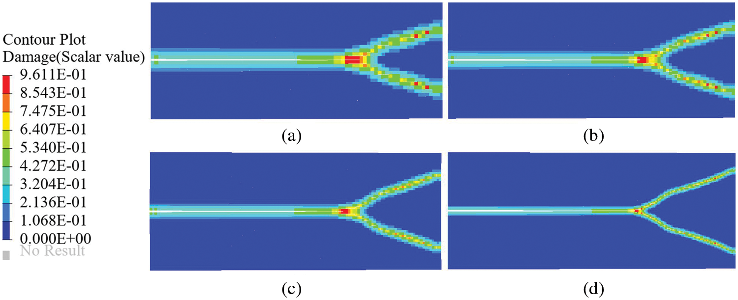
Figure 9: Crack propagation paths of the pre-notched plane under different discretizations. Mesh spacing Δ of (a) 1.25 mm, (b) 1.0 mm, (c) 0.8 mm, and (d) 0.5 mm

4.3 Pre-Notched Cylinder under Internal Pressure

A cylindrical shell [50] subjected to internal pressure in the axial direction and symmetrical pre-notches with bending deformation and membrane deformation is selected to verify the applicability of the proposed PD shell model to the crack propagation of the ordinary shell model. As shown in Fig. 10, the cylinder has a cross-sectional radius of R=5mm, an axial length of L=30mm, and a thickness of t=0.125mm. Two symmetrical pre-cracks are located in the middle of the cylindrical shell axially (Z-axis), with a single crack length of l=4mm. Two cases (a) without and (b) with tear straps are considered. The purpose of installing the tear straps is to restrain the axially propagating crack. The mechanical parameters of the cylinder are taken from literature [50], where Young’s modulus is E=70GPa, Poisson’s ratio is ν=0.3, and the fracture energy is Gc=1.5J/m2, respectively. The displacements in the X-axis and the Y-axis directions at both ends of the cylinder are constrained. Exploiting symmetry, only one-half of the geometry of the cylinder is modeled, and only one layer of material points of the thin cylinder is discretized with a discretization spacing Δ of 0.25 mm. The selected neighborhood horizon is δ=3Δ, and the fracture criterion is as described in Section 3.3 above. The damage clouds of the cylinder in case (a) and case (b) at different force balance stages are shown in Figs. 11 and 12. For the cylinder without tear straps, Fig. 11 shows that a straight crack parallel to the axial direction (Z-axis) of the cylinder propagates toward its ends under the action of internal pressure. As expected, a straight crack propagation path is observed. For the cylinder with tear straps, Fig. 12 shows that the crack propagates in the axial direction in the same way as case (a) until the crack approaches the tear straps, where the direction of crack propagation suddenly changes from axial to circumferential, and the crack branching occurs in the circumferential direction. The presence of tear straps significantly affects the crack propagation path. The damage numerical results of these two cases are the same as those in the literature [50]. Thus, this phenomenon is successfully simulated by the proposed PD shell model.

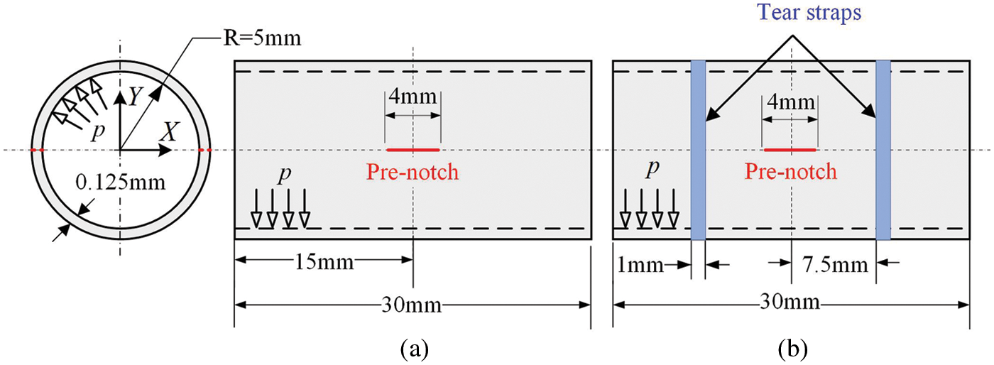
Figure 10: Axially pre-notched thin cylinders under internal pressure (a) without tear straps and (b) with tear straps

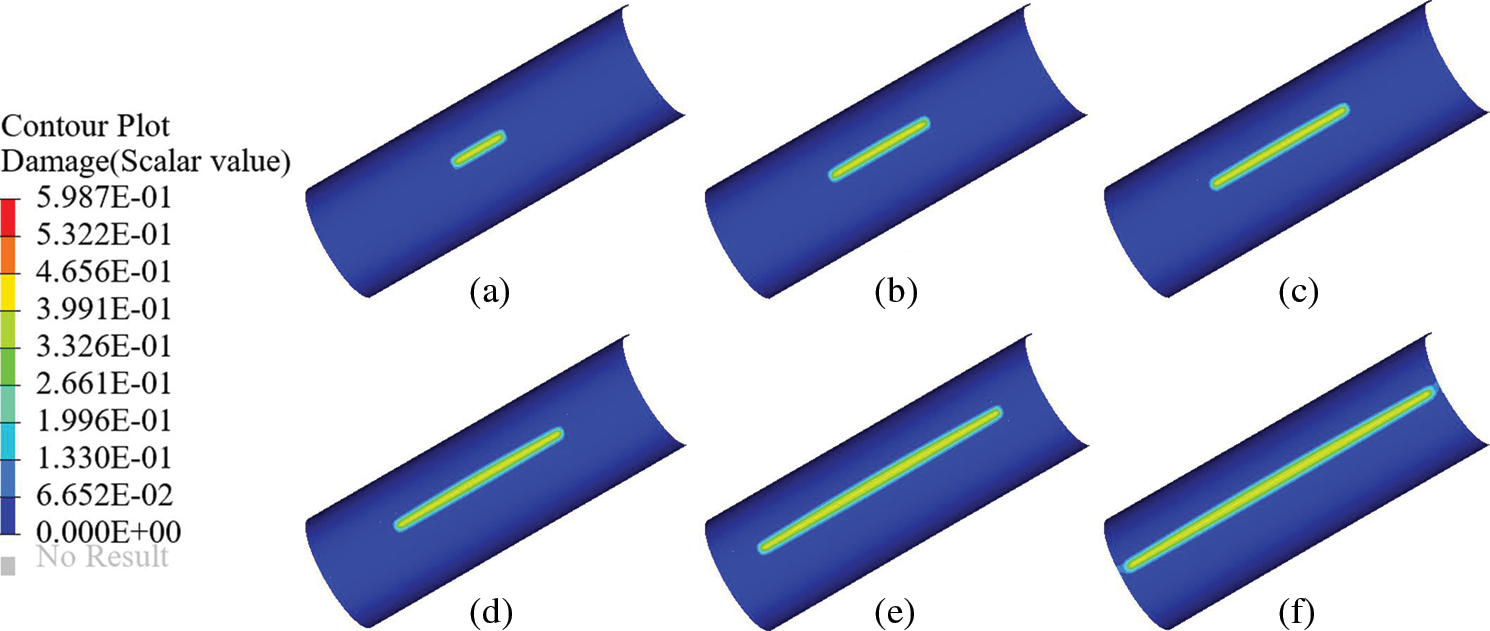
Figure 11: Crack propagation path of the axially pre-notched cylinder without tear straps under internal pressure (a) 0.81 MPa, (b) 0.49 MPa, (c) 0.35 MPa, (d) 0.24 MPa, (e) 0.16 MPa, and (f) 0.095 MPa

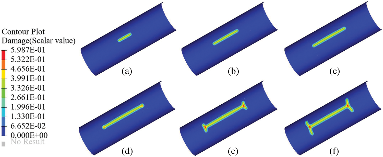
Figure 12: Crack propagation path of the axially pre-notched cylinder with tear straps under internal pressure (a) 0.85 MPa, (b) 0.50 MPa, (c) 0.40 MPa, (d) 0.47 MPa, (e) 0.53 MPa, and (f) 0.46 MPa

4.4 Pre-Notched S-Shaped Curved Shell under Stretching

In this example, an S-shaped curved shell with pre-notches is selected to verify that the proposed PD shell model is applicable to any shell structure and to deal with thin shells with arbitrary cracks. The geometry and dimensions of the long side of the S-shaped curved shell are shown in Fig. 13, which is formed by two arcs tangent to each other with a radius of R = 80 mm. An external load of equal magnitude in opposite directions is exerted on the entire long edge of the shell with a load magnitude of σ=12MPa. Two cases of pre-notches with an angle of (a) 0∘ and (b) 45∘ are considered, as shown in Fig. 13, to observe the crack propagation. The length of the short side of the shell is L=50mm, and a pre-notch with a length of l=10mm exists at the tangent in the middle of the two circular curved surfaces of the thin shell, which is uniformly distributed along the tangent of the curved surface. The material parameters of the thin shell are as follows: Young’s modulus of E=72GPa, Poisson’s ratio of ν=1/3, thickness of t=1mm, and fracture energy of Gc=80J/m2. Only one layer of material points of the S-shaped surface is discretized, with a discretization spacing of Δ=1mm. The neighborhood horizon of the material point is δ=3Δ, and the same fracture criterion as in the previous examples is selected.

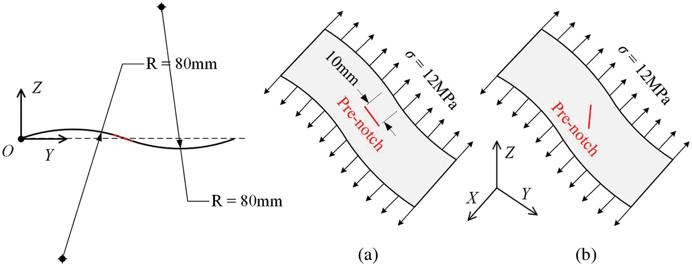
Figure 13: S-shaped shell structure with pre-notch (a) parallel to YZ-plane and (b) 45° with YZ-plane

The damage diagrams of the shell structure at different loading times for two cases are shown in Figs. 14 and 15. Fig. 14 shows that the crack parallel to the YZ-plane propagates in two opposite directions, and the propagation path is roughly parallel to the YZ-plane. However, at the end of the crack propagation, crack bifurcation occurs, and two slightly bifurcated crack propagation paths can be observed. As shown in Fig. 15, the crack at an angle of 45∘ with the YZ-plane first propagates slightly on the shell surface along the pre-notched direction, the direction of crack propagation path changes, and the crack propagates roughly along the YZ-plane in two opposite directions. When the loading time is approximately 21 μs, the first crack bifurcation occurs, and the new crack propagates roughly along the X-axis in two opposite directions. The original and bifurcated cracks propagate simultaneously in the established directions. Eventually, the bifurcation propagation path of the crack can be observed very clearly.

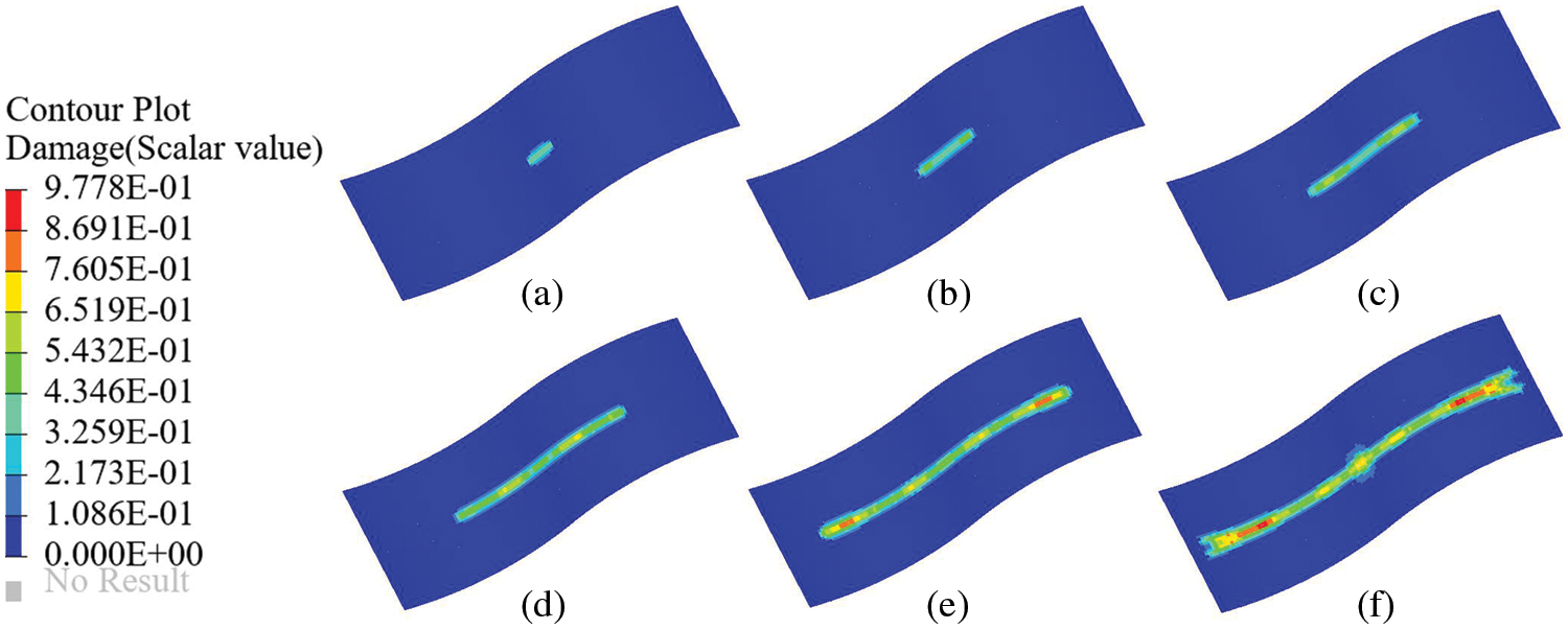
Figure 14: Propagation of crack parallel to the YZ-plane, and the time of (a) 3 μs, (b) 10 μs, (c) 17 μs, (d) 24 μs, (e) 31 μs, and (f) 38 μs

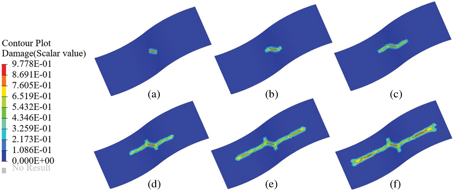
Figure 15: Propagation of the crack at an angle of 45∘ with the YZ-plane, and the time of (a) 3 μs, (b) 10 μs, (c) 17 μs, (d) 24 μs, (e) 31 μs, and (f) 38 μs

5  Conclusion

In this study, a PD shell model based on the micro-beam bond via the homogenization method is presented. First, the deformations of each endpoint of the micro-beam bond are calculated using the interpolation method. Second, the micro-potential energy of the axial, torsional, and bending deformations of the bond can be established from the deformations of endpoints. Finally, the micro moduli of the shell model can be obtained via the equivalence principle of SED. The most critical aspect is the establishment of the conversion relationship between strains of the micro-beam bond and strains of the square element, which can significantly simplify the process of deriving the micro moduli. Different deformations of the micro-beam bond are considered; thus, it is not restricted by material parameters. On the basis of elasticity and small deformations, the 2D plane stress model and the bending model are combined to form a general PD shell model, which is a combination of axial, torsional, and bending deformations. The effectiveness of the proposed PD shell model is demonstrated by several numerical examples. The strain homogenization method used to construct the PD shell model in this study will be applied to the construction of other models in the future, such as anisotropic and large deformation models.

Acknowledgement: The authors wish to express their appreciation to the reviewers for their helpful suggestions which greatly improved the presentation of this paper.

Funding Statement: This work was funded by Project of the National Natural Science Foundation of China (Grant No. 11872017). The support is gratefully acknowledged.

Conflicts of Interest: The authors declare that they have no conflicts of interest to report regarding the present study.

References

 1.  Silling, S. A. (2000). Reformulation of elasticity theory for discontinuities and long-range forces. Journal of the Mechanics and Physics of Solids, 48(1), 175–209. DOI 10.1016/S0022-5096(99)00029-0. [Google Scholar] [CrossRef]

 2.  Kan, X., Yan, J., Li, S., Zhang, A. (2021). On differences and comparisons of peridynamic differential operators and nonlocal differential operators. Computational Mechanics, 68(6), 1349–1367. DOI 10.1007/s00466-021-02072-8. [Google Scholar] [CrossRef]

 3.  D’Antuono, P., Morandini, M. (2017). Thermal shock response via weakly coupled peridynamic thermo-mechanics. International Journal of Solids and Structures, 129, 74–89. DOI 10.1016/j.ijsolstr.2017.09.010. [Google Scholar] [CrossRef]

 4.  Azdoud, Y., Han, F., Lubineau, G. (2013). A morphing framework to couple non-local and local anisotropic continua. International Journal of Solids and Structures, 50(9), 1332–1341. DOI 10.1016/j.ijsolstr.2013.01.016. [Google Scholar] [CrossRef]

 5.  Mikata, Y. (2019). Linear peridynamics for isotropic and anisotropic materials. International Journal of Solids and Structures, 158, 116–127. DOI 10.1016/j.ijsolstr.2018.09.004. [Google Scholar] [CrossRef]

 6.  Chen, H., Lin, E., Liu, Y. (2014). A novel volume-compensated particle method for 2D elasticity and plasticity analysis. International Journal of Solids and Structures, 51(9), 1819–1833. DOI 10.1016/j.ijsolstr.2014.01.025. [Google Scholar] [CrossRef]

 7.  Madenci, E., Oterkus, S. (2016). Ordinary state-based peridynamics for plastic deformation according to von mises yield criteria with isotropic hardening. Journal of the Mechanics and Physics of Solids, 86, 192–219. DOI 10.1016/j.jmps.2015.09.016. [Google Scholar] [CrossRef]

 8.  Pashazad, H., Kharazi, M. (2019). A peridynamic plastic model based on von mises criteria with isotropic, kinematic and mixed hardenings under cyclic loading. International Journal of Mechanical Sciences, 156, 182–204. DOI 10.1016/j.ijmecsci.2019.03.033. [Google Scholar] [CrossRef]

 9.  Ha, Y. D., Bobaru, F. (2011). Characteristics of dynamic brittle fracture captured with peridynamics. Engineering Fracture Mechanics, 78(6), 1156–1168. DOI 10.1016/j.engfracmech.2010.11.020. [Google Scholar] [CrossRef]

10. Ha, Y. D., Bobaru, F. (2010). Studies of dynamic crack propagation and crack branching with peridynamics. International Journal of Fracture, 162(1), 229–244. DOI 10.1007/s10704-010-9442-4. [Google Scholar] [CrossRef]

11. Zhou, X., Wang, Y., Qian, Q. (2016). Numerical simulation of crack curving and branching in brittle materials under dynamic loads using the extended non-ordinary state-based peridynamics. European Journal of Mechanics-A/Solids, 60, 277–299. DOI 10.1016/j.euromechsol.2016.08.009. [Google Scholar] [CrossRef]

12. Chu, B., Liu, Q., Liu, L., Lai, X., Mei, H. (2020). A rate-dependent peridynamic model for the dynamic behavior of ceramic materials. Computer Modeling in Engineering & Sciences, 124(1), 151–178. DOI 10.32604/cmes.2020.010115. [Google Scholar] [CrossRef]

13. Dorduncu, M. (2019). Stress analysis of laminated composite beams using refined zigzag theory and peridynamic differential operator. Composite Structures, 218, 193–203. DOI 10.1016/j.compstruct.2019.03.035. [Google Scholar] [CrossRef]

14. Hu, Y., Yu, Y., Madenci, E. (2020). Peridynamic modeling of composite laminates with material coupling and transverse shear deformation. Composite Structures, 253, 112760. DOI 10.1016/j.compstruct.2020.112760. [Google Scholar] [CrossRef]

15. Diyaroglu, C., Oterkus, E., Madenci, E., Rabczuk, T., Siddiq, A. (2016). Peridynamic modeling of composite laminates under explosive loading. Composite Structures, 144, 14–23. DOI 10.1016/j.compstruct.2016.02.018. [Google Scholar] [CrossRef]

16. Diana, V., Ballarini, R. (2020). Crack kinking in isotropic and orthotropic micropolar peridynamic solids. International Journal of Solids and Structures, 196, 76–98. DOI 10.1016/j.ijsolstr.2020.03.025. [Google Scholar] [CrossRef]

17. Nguyen, C. T., Oterkus, S. (2020). Ordinary state-based peridynamic model for geometrically nonlinear analysis. Engineering Fracture Mechanics, 224, 106750. DOI 10.1016/j.engfracmech.2019.106750. [Google Scholar] [CrossRef]

18. Liu, Z., Bie, Y., Cui, Z., Cui, X. (2020). Ordinary state-based peridynamics for nonlinear hardening plastic materials’ deformation and its fracture process. Engineering Fracture Mechanics, 223, 106782. DOI 10.1016/j.engfracmech.2019.106782. [Google Scholar] [CrossRef]

19. Han, F., Lubineau, G. (2012). Coupling of nonlocal and local continuum models by the arlequin approach. International Journal for Numerical Methods in Engineering, 89(6), 671–685. DOI 10.1002/nme.3255. [Google Scholar] [CrossRef]

20. Han, F., Lubineau, G., Azdoud, Y. (2016). Adaptive coupling between damage mechanics and peridynamics: A route for objective simulation of material degradation up to complete failure. Journal of the Mechanics and Physics of Solids, 94, 453–472. DOI 10.1016/j.jmps.2016.05.017. [Google Scholar] [CrossRef]

21. Han, F., Lubineau, G., Azdoud, Y., Askari, A. (2016). A morphing approach to couple state-based peridynamics with classical continuum mechanics. Computer Methods in Applied Mechanics and Engineering, 301, 336–358. DOI 10.1016/j.cma.2015.12.024. [Google Scholar] [CrossRef]

22. Lubineau, G., Azdoud, Y., Han, F., Rey, C., Askari, A. (2012). A morphing strategy to couple non-local to local continuum mechanics. Journal of the Mechanics and Physics of Solids, 60(6), 1088–1102. DOI 10.1016/j.jmps.2012.02.009. [Google Scholar] [CrossRef]

23. Silling, S. A., Bobaru, F. (2005). Peridynamic modeling of membranes and fibers. International Journal of Non-Linear Mechanics, 40(2–3), 395–409. DOI 10.1016/j.ijnonlinmec.2004.08.004. [Google Scholar] [CrossRef]

24. Gerstle, W., Sau, N., Silling, S. (2007). Peridynamic modeling of concrete structures. Nuclear Engineering and Design, 237(12–13), 1250–1258. DOI 10.1016/j.nucengdes.2006.10.002. [Google Scholar] [CrossRef]

25. O’Grady, J., Foster, J. (2014). Peridynamic plates and flat shells: A non-ordinary, state-based model. International Journal of Solids and Structures, 51(25–26), 4572–4579. DOI 10.1016/j.ijsolstr.2014.09.003. [Google Scholar] [CrossRef]

26. Taylor, M., Steigmann, D. J. (2015). A Two-dimensional peridynamic model for thin plates. Mathematics and Mechanics of Solids, 20(8), 998–1010. DOI 10.1177/1081286513512925. [Google Scholar] [CrossRef]

27. Diyaroglu, C., Oterkus, E., Oterkus, S., Madenci, E. (2015). Peridynamics for bending of beams and plates with transverse shear deformation. International Journal of Solids and Structures, 69, 152–168. DOI 10.1016/j.ijsolstr.2015.04.040. [Google Scholar] [CrossRef]

28. Chowdhury, S. R., Roy, P., Roy, D., Reddy, J. (2016). A peridynamic theory for linear elastic shells. International Journal of Solids and Structures, 84, 110–132. DOI 10.1016/j.ijsolstr.2016.01.019. [Google Scholar] [CrossRef]

29. Taştan, A., Yolum, U., Güler, M. A., Zaccariotto, M., Galvanetto, U. (2016). A 2D peridynamic model for failure analysis of orthotropic thin plates due to bending. Procedia Structural Integrity, 2, 261–268. DOI 10.1016/j.prostr.2016.06.034. [Google Scholar] [CrossRef]

30. Sarego, G., Le, Q. V., Bobaru, F., Zaccariotto, M., Galvanetto, U. (2016). Linearized state-based peridynamics for 2D problems. International Journal for Numerical Methods in Engineering, 108(10), 1174–1197. DOI 10.1002/nme.5250. [Google Scholar] [CrossRef]

31. Yang, Z., Oterkus, E., Nguyen, C. T., Oterkus, S. (2019). Implementation of peridynamic beam and plate formulations in finite element framework. Continuum Mechanics and Thermodynamics, 31(1), 301–315. DOI 10.1007/s00161-018-0684-0. [Google Scholar] [CrossRef]

32. Nguyen, C. T., Oterkus, S. (2019). Peridynamics for the thermomechanical behavior of shell structures. Engineering Fracture Mechanics, 219, 106623. DOI 10.1016/j.engfracmech.2019.106623. [Google Scholar] [CrossRef]

33. Yang, Z., Vazic, B., Diyaroglu, C., Oterkus, E., Oterkus, S. (2020). A kirchhoff plate formulation in a state-based peridynamic framework. Mathematics and Mechanics of Solids, 25(3), 727–738. DOI 10.1177/1081286519887523. [Google Scholar] [CrossRef]

34. Yolum, U., Güler, M. A. (2020). On the peridynamic formulation for an orthotropic mindlin plate under bending. Mathematics and Mechanics of Solids, 25(2), 263–287. DOI 10.1177/1081286519873694. [Google Scholar] [CrossRef]

35. Vazic, B., Oterkus, E., Oterkus, S. (2020). Peridynamic model for a mindlin plate resting on a winkler elastic foundation. Journal of Peridynamics and Nonlocal Modeling, 2(3), 229–242. DOI 10.1007/s42102-019-00019-5. [Google Scholar] [CrossRef]

36. Oterkus, E., Madenci, E., Oterkus, S. (2020). Peridynamic shell membrane formulation. Procedia Structural Integrity, 28, 411–417. DOI 10.1016/j.prostr.2020.10.048. [Google Scholar] [CrossRef]

37. Zhang, Q., Li, S., Zhang, A. M., Peng, Y., Yan, J. (2021). A peridynamic reissner-mindlin shell theory. International Journal for Numerical Methods in Engineering, 122(1), 122–147. DOI 10.1002/nme.6527. [Google Scholar] [CrossRef]

38. Yang, Z., Oterkus, E., Oterkus, S. (2021). Peridynamic modelling of higher order functionally graded plates. Mathematics and Mechanics of Solids, 26(12), 1737--1759. DOI 10.1177/10812865211004671. [Google Scholar] [CrossRef]

39. Zhang, Q., Li, S., Zhang, A. M., Peng, Y. (2021). On nonlocal geometrically exact shell theory and modeling fracture in shell structures. Computer Methods in Applied Mechanics and Engineering, 386, 114074. DOI 10.1016/j.cma.2021.114074. [Google Scholar] [CrossRef]

40. Shen, G., Xia, Y., Hu, P., Zheng, G. (2021). Construction of peridynamic beam and shell models on the basis of the micro-beam bond obtained via interpolation method. European Journal of Mechanics-A/Solids, 86, 104174. DOI 10.1016/j.euromechsol.2020.104174. [Google Scholar] [CrossRef]

41. Shen, G., Xia, Y., Li, W., Zheng, G., Hu, P. (2021). Modeling of peridynamic beams and shells with transverse shear effect via interpolation method. Computer Methods in Applied Mechanics and Engineering, 378, 113716. DOI 10.1016/j.cma.2021.113716. [Google Scholar] [CrossRef]

42. Nguyen-Van, H., Mai-Duy, N., Tran-Cong, T. (2009). An improved quadrilateral flat element with drilling degrees of freedom for shell structural analysis. Computer Modeling in Engineering & Sciences, 49(2), 81–110. DOI 10.3970/cmes.2009.049.081. [Google Scholar] [CrossRef]

43. Foster, J. T., Silling, S. A., Chen, W. (2011). An energy based failure criterion for use with peridynamic states. International Journal for Multiscale Computational Engineering, 9(6), 675--688. DOI 10.1615/IntJMultCompEng.2011002407. [Google Scholar] [CrossRef]

44. Yu, H., Li, S. (2020). On energy release rates in peridynamics. Journal of the Mechanics and Physics of Solids, 142, 104024. DOI 10.1016/j.jmps.2020.104024. [Google Scholar] [CrossRef]

45. Mehrmashhadi, J., Bahadori, M., Bobaru, F. (2020). On validating peridynamic models and a phase-field model for dynamic brittle fracture in glass. Engineering Fracture Mechanics, 240, 107355. DOI 10.1016/j.engfracmech.2020.107355. [Google Scholar] [CrossRef]

46. Sundaram, B. M., Tippur, H. V. (2018). Dynamic fracture of soda-lime glass: A full-field optical investigation of crack initiation, propagation and branching. Journal of the Mechanics and Physics of Solids, 120, 132–153. DOI 10.1016/j.jmps.2018.04.010. [Google Scholar] [CrossRef]

47. Silling, S. A., Askari, E. (2005). A meshfree method based on the peridynamic model of solid mechanics. Computers & Structures, 83(17–18), 1526–1535. DOI 10.1016/j.compstruc.2004.11.026. [Google Scholar] [CrossRef]

48. Zheng, G., Wang, J., Shen, G., Xia, Y., Li, W. (2021). A new quadrature algorithm consisting of volume and integral domain corrections for two-dimensional peridynamic models. International Journal of Fracture, 229(1), 39–54. DOI 10.1007/s10704-021-00540-z. [Google Scholar] [CrossRef]

49. Dipasquale, D., Zaccariotto, M., Galvanetto, U. (2014). Crack propagation with adaptive grid refinement in 2D peridynamics. International Journal of Fracture, 190(1–2), 1–22. DOI 10.1007/s10704-014-9970-4. [Google Scholar] [CrossRef]

50. Kiendl, J., Ambati, M., de Lorenzis, L., Gomez, H., Reali, A. (2016). Phase-field description of brittle fracture in plates and shells. Computer Methods in Applied Mechanics and Engineering, 312, 374–394. DOI 10.1016/j.cma.2016.09.011. [Google Scholar] [CrossRef]

Appendix A. Shape functions for in-plane deformation of the PD shell model

N¯(p,q) is the interpolation function for in-plane deformation, specified as

N¯(p,q)=[N¯1(p,q)N¯2(p,q)N¯3(p,q)N¯4(p,q)]N¯I(p,q)=[N¯I0N¯K1YJ1I−N¯K2YIJ20N¯I−N¯K1XJ1I+N¯K2XIJ200N¯I](I=1,2,3,4)(A1)

p=(X−Xc)/δ,q=(Y−Yc)/δ(−1≤p,q≤1)

The parameters of the bottom right corner mentioned in Eq. (A1) can be defined as

{J1=MOD(I+2,4)+1J2=MOD(I,4)+1K1=J1+4,K2=I+4(A2)

where MOD(x,y) represents the remainder of x divided by y.

Xc and Yc are the coordinates of the square element centroid. The components of N¯I(p,q) can be expressed as

N¯I(p,q)=14(1+pIp)(1+qIq)N¯K(p,q)={116(1−p2)(1+qK−4q)(K=5,7)116(1+pK−4p)(1−q2)(K=6,8)pI=(−1,1,1,−1),qI=(−1,−1,1,1)XIJ=XJ−XI,YIJ=YJ−YI(I=1,2,3,4)(A3)

where K, I, J is an ordered triplet, and the order of value is (5, 1, 2), (6, 2, 3), (7, 3, 4), (8, 4, 1).

Appendix B. Shape functions for bending deformation of the PD shell model

N~(p,q) is the interpolation function for bending deformation, specified as

N~(p,q)=[N~1(p,q)N~2(p,q)N~3(p,q)N~4(p,q)]N~I(p,q)=[N~I(p,q)N~IX(p,q)N~IY(p,q)∂N~I(p,q)δ∂q∂N~IX(p,q)δ∂q∂N~IY(p,q)δ∂q−∂N~I(p,q)δ∂p−∂N~IX(p,q)δ∂p−∂N~IY(p,q)δ∂p](I=1,2,3,4)(B1)

p=(X−Xc)/δ,q=(Y−Yc)/δ(−1≤p,q≤1)

where Xc and Yc are the coordinates of the square element centroid. The components of N~I(p,q) in Eq. (B1) can be expressed as

N~I(p,q)=−18[(1+pIp)(1+qIq)(p2+q2−pIp−qIq−2)]N~IX(p,q)=δ8qI[(1+pIp)(1+qIq)2(qIq−1)]N~IY(p,q)=−δ8pI[(1+pIp)2(1+qIq)(pIp−1)]∂N~I∂p=−18pI(1+qIq)(3p2+q2−qIq−3),∂N~I∂q=−18qI(1+pIp)(p2+3q2−pIp−3)∂N~IX∂p=δ8pIqI(1+qIq)2(qIq−1),∂N~IX∂q=δ8(3qIq−1)(1+pIp)(1+qIq)∂N~IY∂p=−δ8(3pIp−1)(1+pIp)(1+qIq),∂N~IY∂q=−δ8pIqI(1+pIp)2(pIp−1)pI=(−1,1,1,−1),qI=(−1,−1,1,1)(B2)