
 Submit a Paper
 Propose a Special lssue
 Open Access
ARTICLE
The Class of Atomic Exponential Basis Functions EFupn(x,ω)-Development and Application
University of Split, Faculty of Civil Engineering, Architecture and Geodesy, Split, 21000, Croatia
* Corresponding Author:Nives Brajčić Kurbaša. Email:
Computer Modeling in Engineering & Sciences 2023, 135(1), 65-90. https://doi.org/10.32604/cmes.2022.021940
Received 14 February 2022; Accepted 20 May 2022; Issue published 29 September 2022
 View Full Text
 Download PDF
Abstract
The purpose of this paper is to present the class of atomic basis functions (ABFs) which are of exponential type and are denoted by . While ABFs of the algebraic type are already represented in the numerical modeling of various problems in mathematical physics and computational mechanics, ABFs of the exponential type have not yet been sufficiently researched. These functions, unlike the ABFs of the algebraic type , contain the tension parameter , which gives them additional approximation properties. Exponential monomials up to the th degree can be described exactly by the linear combination of the functions . The function for is called the “mother” ABF of the exponential type, i.e., . In other words, the functions are elements of the linear vector space and retain all the properties of their “mother” function . Thus, this paper, in terms of its content and purpose, can be understood as a sequel of the article by Brajčić Kurbaša et al., which shows the basic properties and application of the basis function This paper presents, in an analogous way, the development and application of the exponential basis functions . Here, for the first time, expressions for calculating the values of the functions and their derivatives are given in a form suitable for application in numerical analyses, which is shown in the verification examples of the approximations of known functions.Keywords
Numerical methods are indispensable for the successful simulation of physical and engineering problems. Many different numerical approaches and methods have been proposed in recent decades. The classical methods are the finite element method (FEM), the finite difference method (FDM), the finite volume method (FVM), the boundary element method (BEM), and the discrete element method (DEM) [1–3]. In addition to traditional mesh-based methods, there are many others, such as various meshless methods [4–6].
The choice of the basis functions plays a key role in all numerical methods. The idea of choosing basis functions that correspond to the class of solutions of the problems we are solving has long been accepted, but, in practice, rarely implemented. Polynomials are fundamental to modeling and numerical methods. They provide canonical local approximations to smooth functions and are used extensively in geometric design. Polynomials not only provide very accurate approximations of smooth functions but also guarantee convergence for any continuous function on a compact interval.
Whereas classical polynomials have dominated in the field of numerical analysis, spline-based basis functions [7] play a crucial role in the field of computational geometry. The true popularity of spline functions for numerical analysis was achieved by the introduction of the concept of isogeometric analysis (Hughes et al. [8] and Cottrell et al. [9]). B-splines play an important role in many areas of applied mathematics, computer science, and engineering. Typical applications arise in the approximation of functions and data, automated design and manufacturing, computer graphics, and numerical simulations. This diversity of areas and techniques involved makes B-splines an extremely interesting research topic, which has attracted a growing number of scientists in universities and industry.
In addition to spline functions, relatively lesser-known atomic basis functions have been used in recent times [10–13]. Atomic basis functions can be placed between classical polynomials and spline functions. However, in practice, their use as basis functions is closer to splines or wavelets (see Beylkin et al. [14]). Rvachev et al. [10], in their pioneering work, called these basis functions “atomic” because they span the vector spaces of all three fundamental functions in mathematics: algebraic, exponential, and trigonometric polynomials. The authors of this article have worked intensively on the development and application of ABFs of algebraic type in solving problems of structural mechanics and have therefore demonstrated their significant potential compared to conventional procedures with finite elements. Gotovac [12] systematized the existing knowledge regarding atomic basis functions of algebraic type and transformed them into a numerically appropriate form, especially Fup basis functions as a typical member of the atomic class of basis functions. Gotovac et al. [15] showed the basic possibilities of using atomic functions in structural mechanics and numerical analysis. The work in [16] gives a generalization of atomic functions to the multivariable case. The use of Fup basis functions, which are atomic functions of the algebraic type, has been shown to solve the problem of signal processing [17], the initial value problem [18], the boundary value problems using the Fup Collocation Method [19], the boundary-initial value problems [20], elasto-plastic analysis of prismatic bars subjected to torsion [21], and modeling of groundwater flow and transport problems [22]. Gotovac et al. [23] presented a true multiresolution approach based on the Adaptive Fup Collocation Method (AFCM). Kamber et al. [24] set the foundation for an efficient adaptive spatial procedure by developing a one-dimensional hierarchical Fup (HF) basis functions. The works in [25,26] gave a brief analysis of the current publications regarding ABFs, from the first publications to current ones.
In the mentioned works, the advantage of atomic basis functions of algebraic type, which significantly improve the quality of numerical solutions in relation to classical basis functions, for example, splines and wavelets, is confirmed. The numerical results thus obtained were the motivation for the development of ABF of the exponential type which are wider than algebraic space, moreover algebraic ABFs space is contained in exponential ABFs space.
The numerical modeling of different physical and engineering problems characterized by large local gradients and singularities often presents a challenge in terms of choosing a numerical approach and basis functions. Classic examples of such are the advection–dispersion equation and the heat conduction equation, which describe the transfer of mass and energy, respectively; beams and plates on a flexible foundation; and special problems of loss of stability. For the simulation of such physical problems, exponential basis functions would be a good choice. Improving the quality of numerical analyzes of problems whose solutions have an exponential form is the main motivation of this paper.
The atomic functions of the exponential type have been developed only at the basic level. In [12], the previous knowledge about ABF of the exponential type was presented, which was later expanded and upgraded in [27]. Reference [28], partly resulted from [27], showed the basic properties and application of the maternal basis function
The content of this work is focused on the mathematical background, approximation properties, and applications of exponential basis functions
The following section of the article refers to the description of the ABF class of the algebraic type. The procedure used to generate the class of functions
2 ABFs of the Algebraic Type: Fupn (x)
Atomic Basis Functions (ABFs) are infinitely derivable finite solutions of functional differential equations of the type:
where
The type of finite function
The functions
The functions
Unlike in references [10,11] which define ABFs from Eq. (1), the authors of this paper determine ABFs from their known Fourier transform (FT), and then from their known FT determine everything necessary for their use (e.g., derivatives, integrals, moments, etc.). Namely, we can say that in the “frequency domain” the construction of ABFs becomes more transparent.
The FT of the function
The Fourier transform of the function
Thus, according to Eq. (4), the functions
From the known FT, as is shown similarly for the function
According to Eq. (6), the support of the function
The functional differential equations of the basis functions
where
Solving the functional differential Eq. (8), or Eqs. (4) and (5), is not numerically convenient for calculating the values of the function
The “zeroth” coefficient follows from Eq. (9) and is
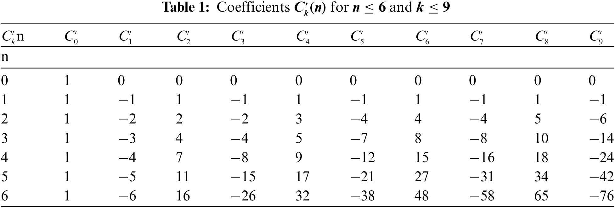
The other coefficients are obtained in the form
The coefficients from Eq. (11) for
The derivatives of the function
where
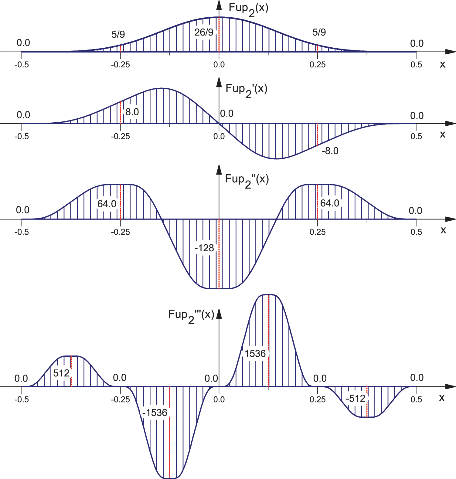
Figure 1: Function
The integrals of the function
3 ABFs of the Exponential Type: EFupn (x, ω)
The functions
3.1 Generating the Fourier Transform of the Function EFupn(x,
The Fourier transform of the atomic basis function
The first from the ABF class of the exponential type
Thus, according to Eq. (14), the Fourier transform of the function
Writing Eq. (15) in an extended form, applying the basic trigonometric relations, and fragmenting the expression thus obtained (omitting the term
The expression in parentheses from Eq. (16) represents the FT of the corresponding exponential spline, while the product from Eq. (16) is the FT of the function
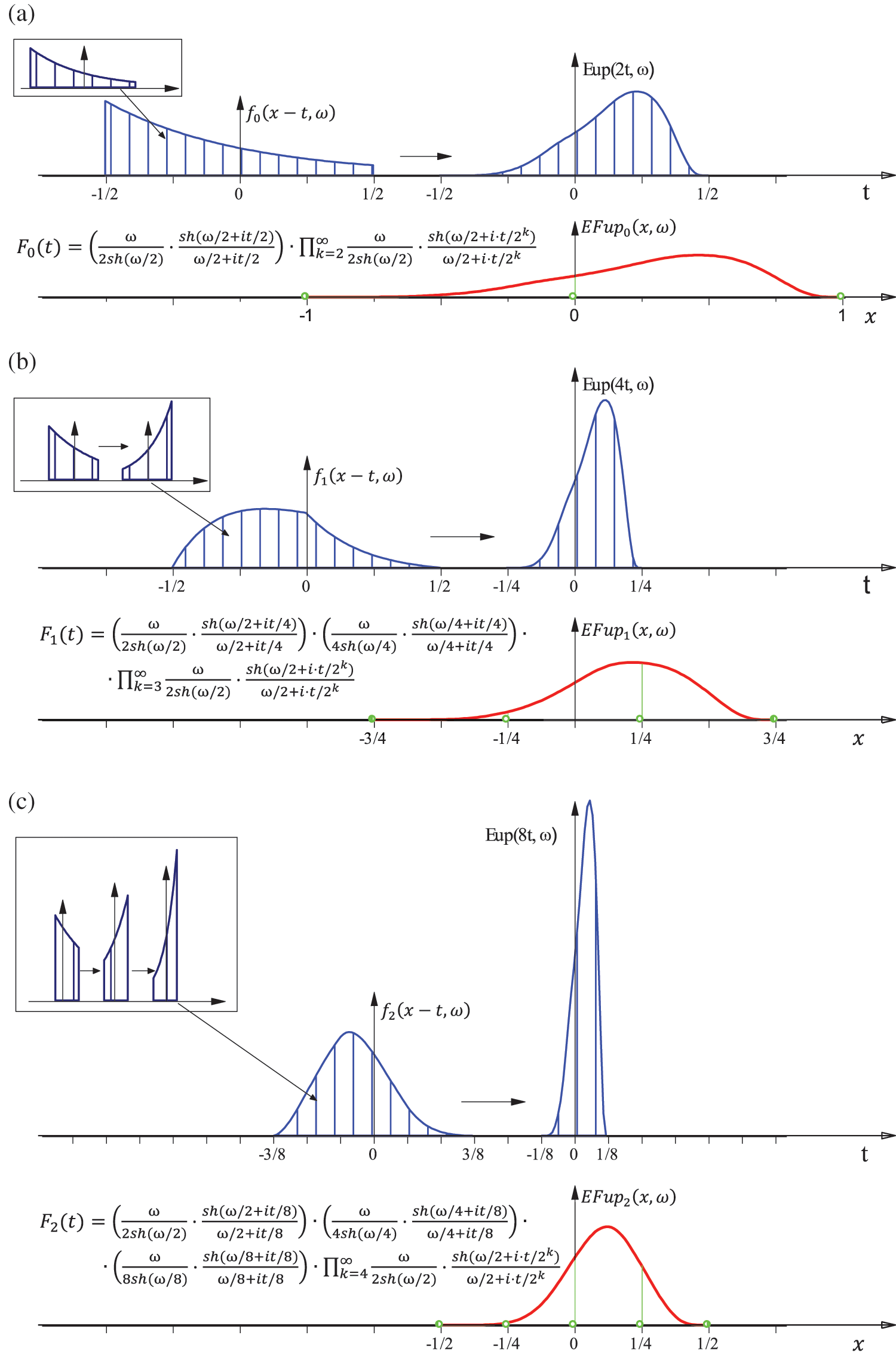
Figure 2: Generating the exponential functions
Thus, analogously to the ABF
where
are the zero-degree exponential splines
When the parameter
Fig. 2 shows a graphical interpretation of Eq. (18) (or Eq. (20)), i.e., the procedure for generating the function
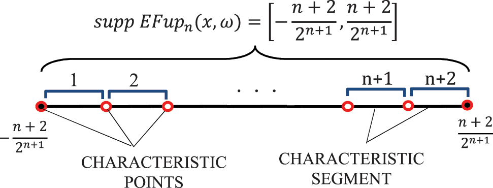
According to Eq. (18), the support of the function
The inverse Fourier transform, i.e., the function
By developing Eq. (21) in the Fourier series, the “original” of the function
Fig. 3 shows the function
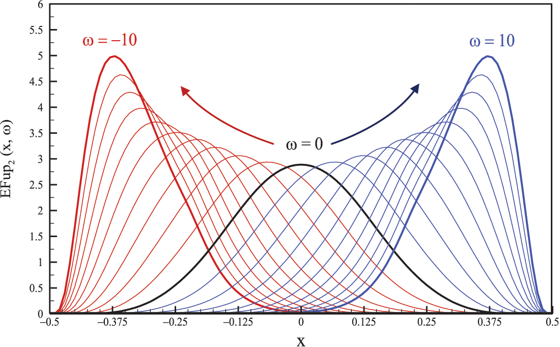
Figure 3: Function
3.2 Functional Differential Equation of the Function EFupn(x,ω)
Analogous to the algebraic ABF
If Eq. (22) is written in the form of exponential functions and multiplied by
where the coefficients are
and
where
In particular, when the value of the parameter
3.3 The Values of the Function EFupn(x, ω) in Characteristic Points
The values of the functions
where
while
However, calculating the integral (27) at arbitrary points
Fig. 4 shows the graphical interpretation of the integral (27) for the basis function
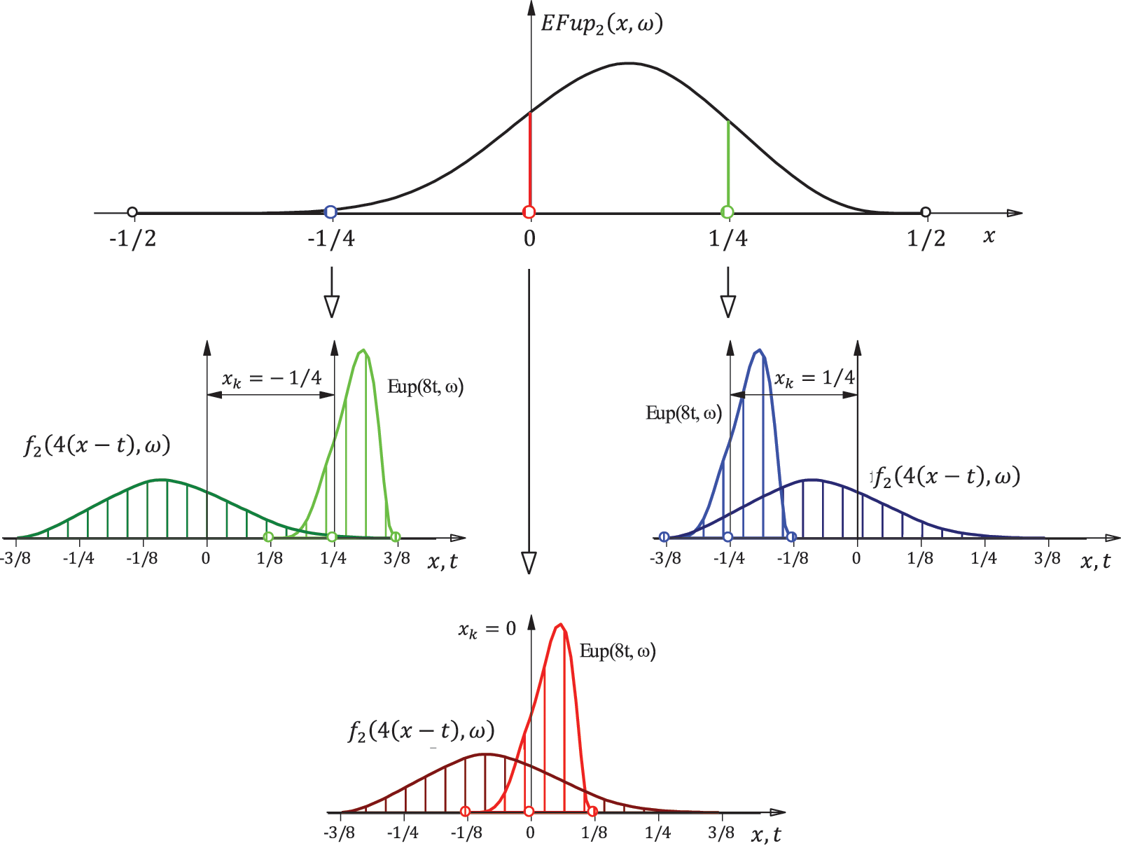
Figure 4: The values of the function
For example, the value of the function
which, when written in exponential form and using the appropriate substitutions after arranging, has the final form:
where
The values at other characteristic points of the function
or the values of the basis functions
As seen in Eqs. (30) and (31), the values of the functions
3.4 EFupn(x, ω) as a Linear Combination of Shifted Eup(x, ω) Functions
The values of the basis functions
where
The “zeroth” coefficient
The other coefficients of the linear combination
For example, for the basis function
or written in characteristic points:
where the values of the basis function
The expression for the “zeroth” coefficient follows directly from the first equation in Eq. (35):
By including the values from (30) and
which corresponds to Eq. (33) for
The “first” coefficient of the linear combination (34) follows from the second equation in Eq. (35) in the form:
By including the coefficient
The expression for the “third” coefficient follows from the third equation in Eq. (35), and so on. By generalizing the presented procedure, a general expression for the coefficients
where the coefficients
Thus, to determine the coefficients
In the limit when
Fig. 5 shows the function
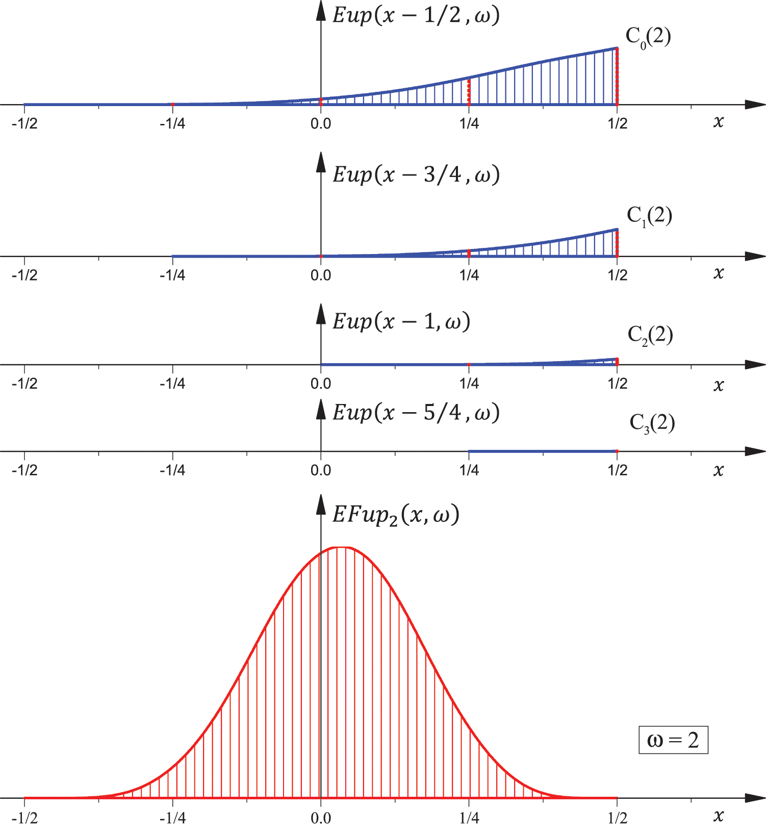
Figure 5: Function
3.5 The Derivatives and Integrals of the Function EFupn(x, ω)
The derivatives of the function
Fig. 6 shows the basis function
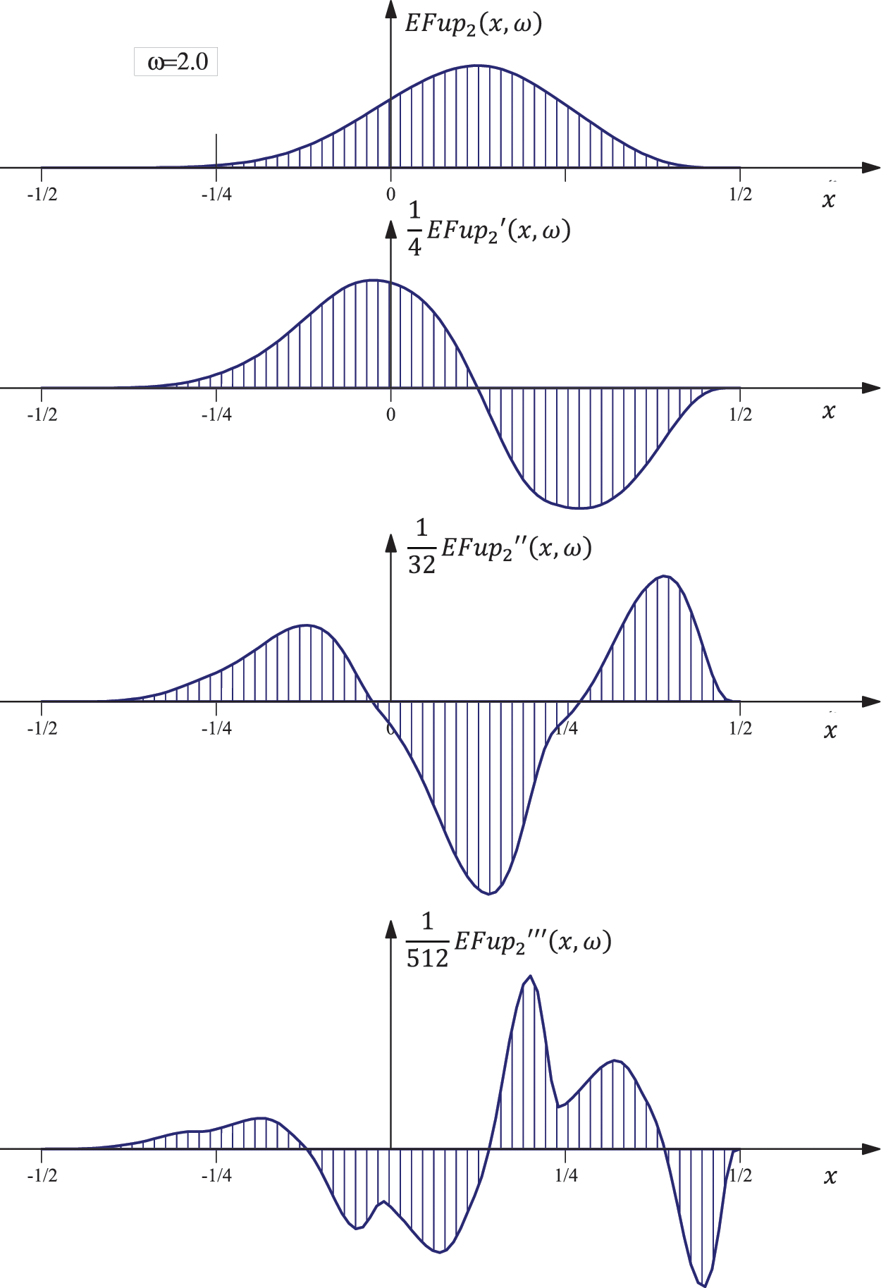
Figure 6: Function
The integrals of the function
3.6 The Connection between the Function EFupn(x, ω) and the Exponential Monomials
Similar to the function
For a linear combination of the basis functions
(offset from each other for the characteristic section
on Eq. (43), the linear combination on the right is annuled.
For example, we show the calculation of the coefficients in the case of the basis function
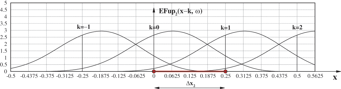
Figure 7: Composition of the
where
or, after reordering:
By introducing the substitution
“Recompositioning” the roots (47) gives the general form of the coefficients
or
The coefficients
For
In general, the exponential monomial
where the coefficients
4 Practical Use of the Exponential ABF EFupn (x, ω)
For practical use we created the efupnM module to calculate the values of the functions
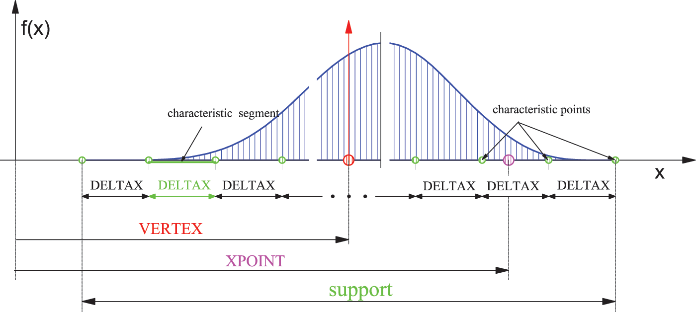
Figure 8: Using the efupnM software module to calculate the values of the basis functions
dummy = efupnM (NFUP, OMEGA, VERTEX, DELTAX, XPOINT, KOD, NMAX),
where:
NFUP =
OMEGA - frequency or tension parameter;
VERTEX - x-local coordinate system coordinates (located in the center of the support);
DELTAX - the real length of the characteristic segment;
XPOINT - the real x-coordinate of the arbitrary point at which the value of the function
KOD - the order of derivation of the function;
NMAX - accuracy parameter (depends on computer characteristics).
4.1 Determination of the Best Frequency in the Function Approximation
The basis functions of the exponential type, such as trigonometric functions, exponential splines, or ABFs of the exponential type, contain the parameter
In this paper, the value of the parameter
Let there be given a function at the section
Using the two characteristic segments of the length
As previously shown in Section 3.6, the linear combination of the basis functions
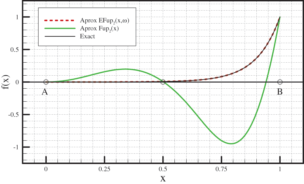
Figure 9: Comparison of the given function (52) and approximations obtained using algebraic and exponential (frequency ω = 10) ABFs for
Thus, the criterion for choosing the parameter’s value is in terms of least squares:
where
Fig. 10 shows the values of the least squares sum (53) for the approximations obtained by the values of the parameter
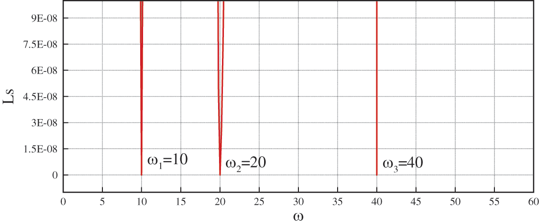
Figure 10: Values of the least squares sum of the approximation obtained by the basis functions
Since the frequency of the given function (52) is known and is
This confirms that the least squares method is a reliable, simple, and optimal choice of criteria for the determination of the value of the parameter ω.
4.2 Example 1: Approximation of a High-Degree Polynomial
An algebraic polynomial of degree 12 is approximated
Unlike the previous example where the value of the parameter
Fig. 11 shows the values of the least squares sum of the approximation obtained by the
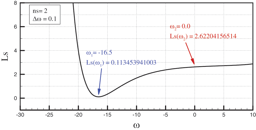
Figure 11: Values of the least squares sum of the approximation obtained by the basis functions
The minimum value of the least squares sum for two characteristic segments was obtained for the approximation using the exponential basis functions
Fig. 12 shows a comparison of the given function (54) with the approximations obtained by the algebraic basis functions
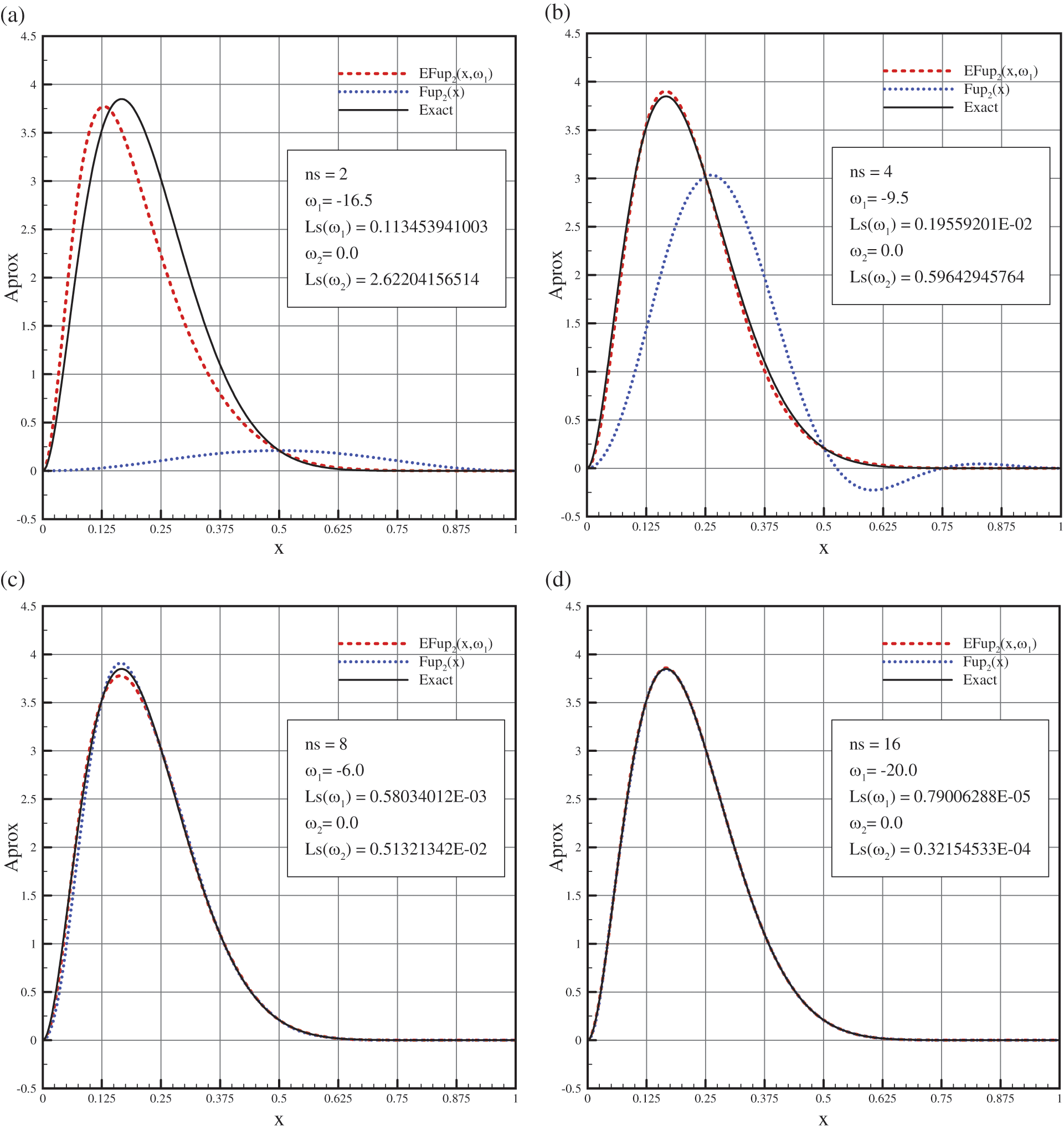
Figure 12: Comparison of the approximations with a given function (54) using the algebraic and exponential ABFs for: (a)
In Figs. 12a and 12b, it can be seen that for a small number of characteristic segments, the approximation by the exponential basis functions
In order to draw a conclusion regarding the character of the convergence of the mentioned numerical approximations to a given function, it is necessary to perform a calculation by increasing the number of segments to a certain desired accuracy of the results. From Fig. 12, it can be seen that the best approximation is achieved using the exponential basis functions with different parameter
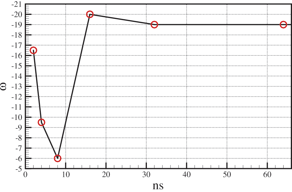
Figure 13: Dependence of the parameter’s
The diagrams in Fig. 14 show, on a logarithmic scale, the relationship between the error expressed over the L2-norm and the segment length
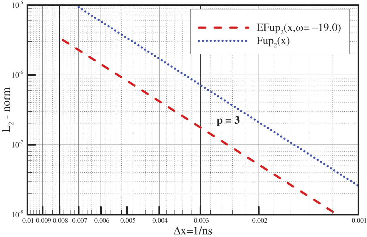
Figure 14: Convergence diagrams of the accuracy of the numerical approximations obtained by the
4.3 Example 2: Approximation of a Sudden Jump Function
The following function on the interval
Fig. 15 shows a comparison of the given function (55) with the approximations obtained by the algebraic basis functions
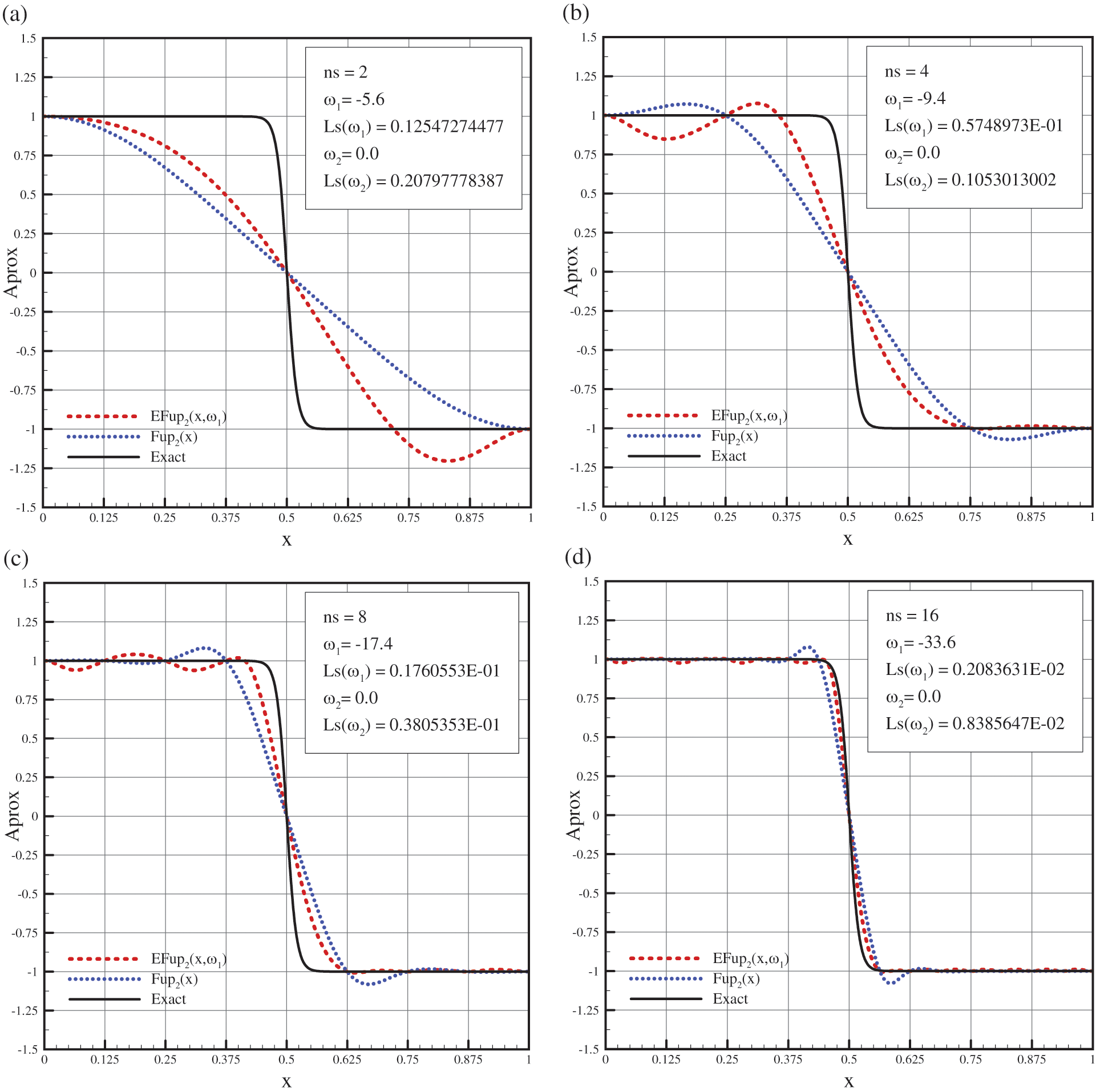
Figure 15: Comparison of the approximations with a given function (55) using the algebraic and exponential basis functions for: (a)
4.4 Example 3: Solving the Differential Equation of Conduction
Let a given differential equation of conduction with corresponding boundary conditions be
with known exact solution of the form
Fig. 16 shows the dependence of the solution of Eq. (56) on the parameter
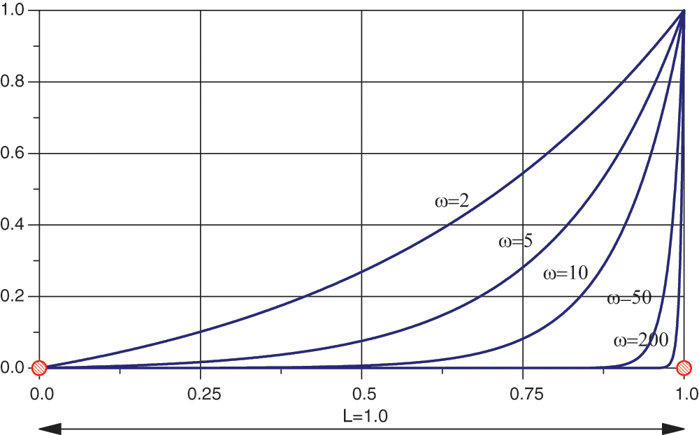
Figure 16: Dependence of the exact solution of the conduction problem (56) on the frequency
Fig. 17 compares the exact solution (57) of the conduction problem (56) with the solutions obtained using the basis functions
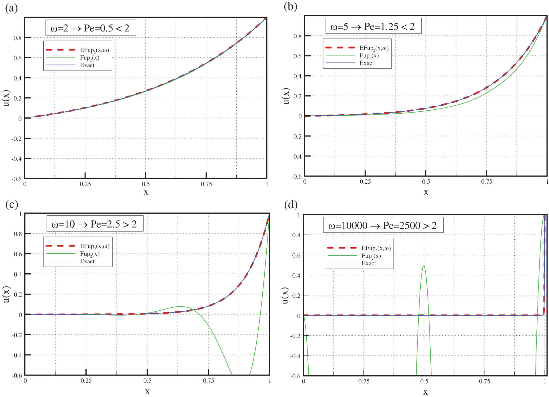
Figure 17: Comparison of the numerical solutions of Eq. (56) obtained by the
Approximation using the basis functions of the algebraic type is limited by the Peclet number
In Fig. 17a for
The current knowledge regarding algebraic atomic basis functions
In the examples of the approximations of given functions, namely, a high-degree algebraic polynomial representing an asymmetric function and functions with a sudden jump, the exponential basis functions
Algebraic atomic basis functions have been used for many years to solve various numerical problems, and their advantage over other basis functions has become unquestionable. The ABFs of the exponential type show even better approximation properties, as demonstrated in this paper. The only question that still remains open is the choice of the value of the tension parameter ω. As with exponential splines, this complex issue requires further research both in one-dimensional problems and in the higher dimensions of space. In this paper, for the parameter selection criterion, we used the least squares sum, which proved to be simple and reliable. However, a disadvantage was the additional CPU time required to simultaneously solve the system of equations for the purpose of obtaining the approximations for different values of the parameter
Our further research should include an improvement of the procedure for finding the optimal value of the tension parameter. The natural sequence of development and application of the ABF of the exponential type leads to 2D and 3D numerical analysis. The advantage of ABF of the exponential type can be suitable for the application of adaptive procedures in the problems of computational mechanics.
Funding Statement: This research is partially supported through Project KK.01.1.1.02.0027, a project co-financed by the Croatian Government and the European Union through the European Regional Development Fund-the Competitiveness and Cohesion Operational Programme.
Conflicts of Interest: The authors declare that they have no conflicts of interest to report regarding the present study.
References
1. Zienkiewicz, O. C., Taylor, R. L. (2002). The finite element method. Oxford: Butterworth-Heinemann. [Google Scholar]
2. Sauter, S. A., Schwab, C. (2011). Boundary element methods. Berlin, Heidelberg: Springer. [Google Scholar]
3. Tavarez, F. A., Plesha, M. E. (2007). Discrete element method for modelling solid and particulate materials. International Journal for Numerical Methods in Engineering, 70(4), 379–404. DOI 10.1002/(ISSN)1097-0207. [Google Scholar] [CrossRef]
4. Belytschko, T., Krongauz, Y., Organ, D., Fleming, M. A., Krysl, P. (1996). Meshless methods: An overview and recent developments. Computer Methods in Applied Mechanics and Engineering, 139(1–2), 3–47. DOI 10.1016/S0045-7825(96)01078-X. [Google Scholar] [CrossRef]
5. Liu, G. R., Gu, Y. T. (2005). An introduction to meshfree methods and their programming. Dordrecht: Springer. [Google Scholar]
6. Fries, T. P., Matthies, H. G. (2004). Classification and overview of meshfree methods. Brunswick: Institute of Scientic Computing Technical University Braunschweig. [Google Scholar]
7. Hölling, K., Hörner, J. (2013). Approximation and Modeling with B-splines. Philadelphia: Siam. [Google Scholar]
8. Hughes, T., Cottrell, J., Bazilevs, Y. (2005). Isogeometric analysis: CAD, finite elements, nurbs, exact geometry and mesh refinement. Computer Methods in Applied Mechanics and Engineering, 194(39), 4135– 4195. DOI 10.1016/j.cma.2004.10.008. [Google Scholar] [CrossRef]
9. Cottrell, J. A., Hughes, T. J. R., Bazilevs, Y. (2009). Isogeometric analysis toward intergration of CAD and FEA. Wiley. [Google Scholar]
10. Rvachev, V. L., Rvachev, V. A. (1971). On a finite function. Doklady Akademii Nauk Ukrainian SSR, A(6), 705–707. [Google Scholar]
11. Rvachev, V. L., Rvachev, V. A. (1979). Non-classical methods for approximate solution of boundary-value problems. Kiev: Naukova dumka. [Google Scholar]
12. Gotovac, B. (1986). Numerical modelling of engineering problems by smooth finite functions (Ph.D. Thesis). University of Split, Split (in Croatian). [Google Scholar]
13. Kravchenko, V. F. (2003). Lectures on the theory of atomic functions and their some applications. Moscow: Radiotechnika. [Google Scholar]
14. Beylkin, G., Keiser, J. M. (1997). On the adaptive numerical solution of nonlinear partial differential equations in wavelet bases. Journal of Computational Physics, 132(2), 233– 259. DOI 10.1006/jcph.1996.5562. [Google Scholar] [CrossRef]
15. Gotovac, B., Kozulić, V. (1999). On a selection of basis functions in numerical analyses of engineering problems. International Journal for Engineering Modelling, 12(1–4), 25–41. [Google Scholar]
16. Kolodiazhny, V. M., Rvachev, V. A. (2007). Atomic functions: Generalization to the multivariable case and promising applications. Cybernetics and Systems Analysis, 43(6), 893–911. DOI 10.1007/s10559-007-0114-y. [Google Scholar] [CrossRef]
17. Kravchenko, V. F., Basarab, M. A., Perez-Meana, H. (2001). Spectral properties of atomic functions used in digital signal processing. Journal of Communications Technology and Electronics, 46, 494–511. [Google Scholar]
18. Gotovac, B., Kozulić, V. (2002). Numerical solving of initial-value problems by Rbf basis functions. Structural Engineering and Mechanics, 14(3), 263–285. DOI 10.12989/sem.2002.14.3.263. [Google Scholar] [CrossRef]
19. Kozulić, V., Gotovac, B. (2000). Numerical analyses of 2D problems using Fupn(x,y) basis functions. International Journal for Engineering Modelling, 13(1–2), 7–18. [Google Scholar]
20. Gotovac, H., Kozulic, V., Gotovac, B. (2010). Space-time adaptive fup multi-resolution approach for boundary-initial value problems. Computers, Materials & Continua, 15(3), 173–198. DOI 10.3970/cmc.2010.015.173. [Google Scholar] [CrossRef]
21. Kozulic, V., Gotovac, B. (2011). Elasto-plastic analysis of structural problems using atomic basis functions. Computer Modeling in Engineering & Sciences, 80(4), 251–274. DOI 10.3970/cmes.2011.080.251. [Google Scholar] [CrossRef]
22. Gotovac, H., Andricevic, R., Gotovac, B., Kozulic, V., Vranjes, M. (2003). An improved collocation method for solving the Henry problem. Journal of Contaminant Hydrology, 64(1), 129–149. DOI 10.1016/S0169-7722(02)00055-4. [Google Scholar] [CrossRef]
23. Gotovac, H., Cvetkovic, V., Andricevic, R. (2009). Adaptive Fup multi-resolution approach to flow and advective transport in highly heterogeneous porous media: Methodology, accuracy and convergence. Advances in Water Resources, 32(6), 885–905. DOI 10.1016/j.advwatres.2009.02.013. [Google Scholar] [CrossRef]
24. Kamber, G., Gotovac, H., Kozulić, V., Malenica, L., Gotovac, B. (2020). Adaptive numerical modeling using the hierarchical Fup basis functions and control volume isogeometric analysis. International Journal for Numerical Methods in Fluids, 92(10), 1437–1461. DOI 10.1002/fld.4830. [Google Scholar] [CrossRef]
25. Kravchenko, V. F., Kravchenko, O. V., Konovalov, Y. Y., Budunova, K. A. (2020). Atomic functions theory: History and modern results: Dedicated to the pioneer of atomic functions theory V. L. Rvachev invited paper. IEEE Ukrainian Microwave Week, 43, 619–623. DOI 10.1109/UkrMW49653.2020.9252684. [Google Scholar] [CrossRef]
26. Kravchenko, V. F., Kravchenko, O. V., Pustovoit, V. I., Churikov, D. V., Volosyuk, V. K. et al. (2016). Atomic functions theory: 45 years behind. 9th International Kharkiv Symposium on Physics and Engineering of Microwaves, Millimeter and Submillimeter Waves (MSMW), pp. 1–4. DOI 10.1109/MSMW.2016.7538216. [Google Scholar]
27. Brajčić Kurbaša, N. (2016). Exponential atomic basis functions: Development and application (Ph.D. Thesis). University of Split, Split (in Croatian). [Google Scholar]
28. Brajčić Kurbaša, N., Gotovac, B., Kozulić, V. (2016). Atomic exponential basis function Eup(x,ω)-development and application. Computer Modeling in Engineering & Sciences, 111(6), 493–530. DOI 10.3970/cmes.2016.111.493. [Google Scholar] [CrossRef]
Cite This Article
 Copyright © 2023 The Author(s). Published by Tech Science Press.
This work is licensed under a Creative Commons Attribution 4.0 International License , which permits unrestricted use, distribution, and reproduction in any medium, provided the original work is properly cited.
 Downloads
 Citation Tools