A Two-Step Algorithm to Estimate Variable Importance for Multi-State Data: An Application to COVID-19

1  Introduction

In longitudinal health studies, a patient may experience a sequence of clinical progression events. For instance, the local recurrence may be followed by a distant recurrence and then death [1]. Also, in the renal transplantation process of patients with end-stage kidney disease, renal allograft failure is considered an intermediate event that can affect the whole survival of the patient [2]. For another instance, the state of the COVID-19 patients who are admitted to the intensive care unit (ICU) at the time of admission can influence their survival time. A patient may need invasive or non-invasive ICU ventilation and extracorporeal membrane oxygenation and may be discharged from the hospital or die eventually [3]. Moreover, the need for ICU before death or discharge from the hospital among COVID-19 patients who are admitted to the ward could be another state. In such studies, the progression of the disease is considered as a multi-state process, and multi-state models (MSM) are used to assess the impact of different covariates on the transition between different health states [1,4]. Ferrer et al. [1] developed a multi-state model for the analysis of prostate cancer. Beesley et al. [4] also applied the multi-state approach for modeling the progression of prostate cancer.

One main objective in the MSM framework is variable selection, where attempts are made to identify the risk factors associated with the transition hazard rates or probabilities of the disease progression. The classic approach is to use stepwise methods, where steps are taken by sequentially adding (forward) or removing (backward) variables at each step. However, the stepwise method suffers from some drawbacks, such as instability of the selected variables. In the context of MSMs, few attempts have been made at the variable selection. For example, Dang et al. [5] suggested L1-Regularized multi-state models using a Least Absolute Shrinkage and Selection Operator (LASSO) penalty for parameter estimation and variable selection, simultaneously. The LASSO method has several advantages for variable selection, including sparseness avoiding overfitting and a lower burden of computations. It is also applicable in the presence of a large number of covariates. Nevertheless, the selected model by the LASSO is unstable in terms of selected features. Moreover, for a set of highly correlated features, the LASSO selects one of them randomly. Penalized methods neglect the interaction between variables and their complex relationships or their unknown functional form. Most importantly, these techniques were unable to provide a quantitative assessment of their significance [6]. While some of the features measured in a study may be associated with the sojourn times in the entry states of each transition, they may have different degrees of importance, and some of them may be more important for some transitions than others [7]. The variable importance can be estimated as a real-valued parameter using an optimal estimating function [8].

In the context of COVID-19, several studies have investigated factors associated with various outcomes using machine learning models through variable importance. For example, Stachel et al. utilized machine learning methods for variables associated with mortality among COVID-19 patients [9]. Also, Snider et al. investigated variables affecting mortality in COVID-19 patients using artificial intelligence methods [10]. However, most of these studies considered binary outcomes such as survival or death. In various studies, random survival forest has been used to predict mortality in hospitalized COVID-19 patients. They considered time to hospital discharge and mortality as the outcomes of interest and competing risks, respectively. More complex structures were also considered by some authors. Hazard et al. [11] considered a multistate structure for joint analysis of the duration of ventilation, length of intensive care, and mortality of COVID-19 patients. To our knowledge, no study has dealt with estimating variable importance in multi-state data structures such as COVID-19 data.

Breiman [12] introduced the random forest technique for classification and regression problems, where it has been widely used for variable selection. Gradient boosting [13] is also a commonly used method for variable selection, showing satisfactory performance in many problems. Negassa et al. [14] investigated model selection in tree-structured subgroup analysis using the RECursive Partition and Amalgamation algorithm. They found that there is no single model selection criterion with uniformly superior performance, and they proposed a two-stage approach for model selection with promising performance in variable selection. Recently, Duan et al. [6] proposed a machine learning-based approach to estimate variable importance using martingale and deviance residuals and their standardized counterparts which resulted in promising performances based on simulation studies. In the present study, we proposed a two-step algorithm to estimate the importance of variables for multi-state data based on three different machine learning approaches: random forest, gradient boosting, and neural network as the most widely used method. Our main contribution to this study is to extend the proposed approach to multi-state data to estimate the variable importance. The remaining sections of this paper are organized as follows: In Section 2, we describe the multi-state model and its related residuals. In Section 3, we define three risk indices based on the residuals mentioned in Section 2. In Section 4, we describe our proposed two-step algorithm to evaluate the variable’s importance for multi-state data and introduce the loss function criteria to compare the performance of different methods. In Section 5, the performance of our algorithm is evaluated via simulation studies, and we apply our method to the COVID-19 data set through an illness-death multi-state model, and a brief discussion is finally given in Section 5.

2  Methods

2.1 Multi-State Model

A multi-state model is a stochastic process ({X(t),t∈ς}) with a finite state space S={0,1,…,p}, where ς=[0,τ] for τ≤+∞. The multi-state process is assumed to be continuous-time with the right-continuous sample paths, X(t+)=X(t). The transition probabilities are given as follows:

Phk(s,t)=P(X(t)=k|X(s)=h,χs−),

for h,k∈S, s,t∈ς,s≤t, and χs be a σ-algebra that stands for everything that happened up to time s. Then, the transition intensities are defined as follows:

λhk(t)=limΔt→0Phk(t,t+Δt|χs−)Δt.

Suppose, there are n subjects and let Ti=(Ti1,…,Timi) represents the vector of the mi≥1 observed transition times for the ith subject, with Tir<Ti(r+1), r∈{1,…,mi}. When the last observed state is an absorbing state (i.e., a state that once entered cannot be never left; e.g., death), then the ith subject will experience mi direct transitions. Otherwise, Timi is equal to right censoring time Ci and there are mi−1 direct transitions.

The counting process for the subject i (i=1,…,n) can be defined as (a multivariate counting process) by {Nhki(t),h,k∈S,h≠k,t≤Ci} counting the number of direct transitions from the state h to the state k for the subject i over the interval [0,t] and Ci(≤τ). The intensity function for the subject i based on the Cox regression model, by using counting process formulation of the model, is given as follows:

λhki(t)=limΔt→0P{Nhki(t,t+Δt)=1|χs−}Δt=Yhi(t)λhk0(t)exp⁡{βhkTZhki(t)}.(1)

Here, Yhi(t)=I(Xi(t−)=h) is an indicator specifying whether Xi(.) is in the state h at time t− (some h and k combinations may not be possible). Specifically, Yhi(t)=1 means that the individual i is at risk for transition from h to k immediately before time t. The Nhki(t) only jumps when Yhi(t)=1. Also, in the above equation λhk0(.) is the baseline intensity function, and Zhki(t) is the vector of predictors associated with the vector of coefficients βhk for the transition from h to k.

Note that, under the Markov assumption, future evolution of the process only depends on the current state and, therefore, χs− has been omitted from the formulas.

2.2 Risk Indices

2.2.1 Martingale Residuals

Using the Doob–Meyer decomposition [15], in multi-state models, the martingale residual for the subject i on the time interval of [0,t] is defined as follows:

Mhki(t)=Nhki(t)−Λhki(t)=Nhki(t)−∫0tYhi(u)exp⁡{βhkTZhki(u)}dΛhk0(u).

In the above equation, Λhki(t) represents the cumulative intensity function and is a predictable process called the compensator of Nhki(t). Also, Λhk0(t)=∫0tλhk0(u)du indicates the cumulative baseline intensity function. The βhk and Λhk0(t) are unknown parameters that should be estimated. Let β⌢hk and Λ⌢hk0(t) represent the maximum likelihood estimator of βhk [16,17] and the Breslow estimator of Λhk0(t) [17,18], respectively. Then, the martingale residual for the transition h→k is defined as follows:

M⌢hki(t)=Nhki(t)−∫0tYhi(u)exp⁡{β⌢hkTZhki(u)}dΛ⌢hk0(u).

In the multi-state data, suppose that the last observed time of transition from the state h to the state k (h → k) for the subject i is called τki, (the minimum of the administrative censoring time Ca, the individual censoring time (loss to follow-up) Ci and the time of transition to the state k, ∀k∈{2,…,mi}). Therefore, the martingale residual for the subject i at time τki has the following form:

M⌢hki(τki)=Nhki(τki)−exp⁡{β⌢hkTZhki}Λ⌢hk0(τki).(2)

Note that, we use M⌢hki to represent M⌢hki(τki).

2.2.2 Deviance

The deviance defined in Therneau et al. [19] is as follows:

D = 2{log likelihood (saturated model)-log likelihood (β⌢)}.

The saturated model is a model with a parameter for every observation. Here, we extend the definition of the deviance for univariate survival data to the multi-state data. Under mild regularity conditions, the log-likelihood contribution for each individual can be obtained using counting process theory as follows:

Li=∑r=1mi[∫0Tirlog⁡(λXi(Tir),Xi(Tir),i(t))dNhki(t)−∫Ti(r−1)TirλXi(Ti(r−1)),Xi(Tir),i(t)Yhi(t)dt].

Note that λhhi(t)=−Σkλhki(t) for k≠h, and δir is a transition indicator (for the subject i) which equals one if a direct transition is observed at time Tir and zero otherwise.

Then, the definition of deviance for multi-state data with the intensity function in Eq. (1), which is an extension of the deviance provided by Therneau et al. [19] for survival data, is as follows:

Dhk=2supγhk∑i=1n[∫Yhi(t){γhkiTZi−β⌢hkTZi}dNhki(t)−∫Yhi(t){exp⁡(γhkiTZi)−exp⁡(β⌢hkTZi)}dΛhk0(t)].(3)

Let γhki be the per-subject estimates of βhk. By taking the first derivation of the above summation part with respect to γhki and setting it equal to 0, we have:

∫Yhi(t)exp⁡(γhkiTZi)dΛhk0(t)=∫dNhki(t).(4)

By subtracting Eqs. (3) and (4), Dhki has the following form:

Dhki=−2[Mhki+Nhki(t)log⁡(Nhki(t)−MhkiNhki(t))].

As mentioned before, we supposed τki is the observed time of transition to the state k (for the transition from state h to state k). Therefore, the deviance at time τki has the following form:

Dhki=−2[M⌢hki+Nhki(τki)log⁡(Nhki(τki)−M⌢hkiNhki(τki))].(5)

Note that Nhki(τki)≠0, and Dhki=−2M⌢hki when Nhki(τki)=0.

2.2.3 Deviance Residuals

The deviance residuals are defined as follows:

Dhkires=sign(M⌢hki)×Dhki.(6)

The deviance residual Dhkires is equal to zero if the martingale residual is zero (Mhki=0). The variables are considered to be fixed over time (not time-dependent). In this paper, the martingale residuals, the deviances, and the deviance residuals are called risk indices.

2.3 Variable Importance for Multi-State Data

In this section, we introduce an algorithm to evaluate the variable’s importance for multi-state data. Therneau et al. [19] mentioned that using martingale residuals from a null Cox model as the input of classification and regression trees worked well for survival data. Then, Duan et al. [6] extended their proposed algorithm to recurrent event data. Here, we extend their approach to multi-state data.

2.3.1 Two-Step Variable Selection Algorithm

The proposed algorithm has two steps. In the first step, a null multi-state model is fitted as follows:

λhki(t)=Yhi(t)λhk0(t).

This model does not include any variables, and only the baseline intensity functions should be estimated, which can be estimated using the Breslow estimator [17,18]. Then, the martingale residuals, the deviances, and the deviance residuals are obtained as three risk indices for each subject. For a multi-state model with three states (depicted in Fig. 1) (mi=3), the martingale residuals are defined as follows:

M⌢12i(τ2i)=N12i(τ2i)−Λ⌢120(τ2i),

M⌢13i(τ3i)=N13i(τ3i)−Λ⌢130(τ3i),

M⌢23i(τ3i∗)=N23i(τ3i∗)−Λ⌢230(τ3i∗),

where τ2i=Ti2 is the observed time of the transition from the state 1 to the state 2, τ3i=Ti3 is the observed time of the transition from the state 1 to the state 3, and τ3i∗=Ti3−Ti2 is the observed time of the transition from the state 2 to the state 3. Then, the deviances are as follows:

D12i=−2[M⌢12i+N12i(τ2i)log⁡(N12i(τ2i)−M⌢12iN12i(τ2i))],

D13i=−2[M⌢13i+N13i(τ3i)log⁡(N13i(τ3i)−M⌢13iN13i(τ3i))],

D23i=−2[M⌢23i+N23i(τ3i∗)log⁡(N23i(τ3i∗)−M⌢23iN23i(τ3i∗))],

and the deviance residuals are defined as follows:

D12ires=sign(M⌢12i)×D12i,

D13ires=sign(M⌢13i)×D13i,

D23ires=sign(M⌢23i)×D23i.

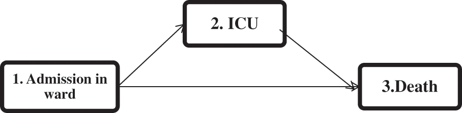
Figure 1: The multi-state representation of the disease progression of COVID-19 hospitalized patients

In the second step, the random forest, the gradient boosting, and the neural network methods are applied to the risk indices generated in the first step to evaluate the importance of each variable in different transitions.

2.4 Machine Learning Models

2.4.1 Random Forest

The random forest method is a supervised ensemble learning algorithm developed by Brieman in 2001. It is constructed by combining several decision tree algorithms to create solutions for complex problems. In this method, a series of simple unpruned regression trees are constructed by using random bootstrapped samples that are obtained from the original data sample. The results of the simple trees are then accumulated to produce a final prediction of the response for the subjects in regression problems, which is the average of the predictions given by all trees. In the random forest algorithm, in the first step, for b = 1 to B, a bootstrapped sample K* of size N (the original sample size) is drawn from the training data. Each tree (Tb), in the random forest, is grown for the bootstrapped data by repeating the following recursive steps for each of the terminal nodes in the tree: a) A set of m variables is randomly selected from a set of p original variables; b) the best variable/split-point is selected from the set of m variables chosen in Step (a); and c) the node is split into two daughter nodes. These three steps are repeated until the minimum predefined node size is achieved (nmin). In the second step, the output of all trees (B) is aggregated. A prediction for a new observation is obtained by calculating 1B∑1BTb(x).

2.4.2 Gradient Boosting Machine

Gradient boosting machines (GBMs) consist of a group of powerful machine-learning methods with substantial accomplishments in many practical applications. GBMs can be very adaptable to the needs of the application. The boosting works based on sequentially adding new models to the ensemble, so that in each particular iteration, “a new weak, base-learner model is trained with respect to the error of the whole ensemble learnt so far” [20]. A GBM has been established to connect boosting with a statistical framework [21–23], which provides the required justification for the hyperparameters in the model and the methodological foundation for developing further gradient boosting models [20].

In GBMs, successive new models are fitted based on the chosen learning technique; so that more accurate estimates of the outcome are produced. The main idea underlying this algorithm is to create “the new base-learners to be maximally correlated with the negative gradient of the loss function, associated with the whole ensemble” [20]. The loss functions used can be researcher-defined or standard loss functions derived through trial and error in the past.

2.4.3 Neural Network

Artificial neural networks (ANNs) are machine learning methods that consist of an input layer of neurons (or nodes, units), at least one hidden layer of neurons, and a layer of output neurons. Connections between layers are illustrated by numeric values (e.g., weights) through activation functions. The most widely used form of ANN is the multi-layer perceptron, where the data flows in a forward direction from the input layer to the output layer. So, the neurons are trained with the back propagation learning algorithm. In this study, the regression weights were estimated using a tangent hyperbolic activation function and an identity activation function, which provided better results than other settings [24].

2.5 Performance Measurement

Here, the loss function (introduced by Cox [17,18]) was considered to assess the performance of the different variable importance evaluation methods for multi-state data. Suppose that there are q standardized covariates xhk1,…,xhkq for the transition from state h to state k that are associated with the coefficients ηhk1,…,ηhkq, respectively. The absolute values of the coefficients are related to their importance, such that, for the transition h→k, if the ranks of the absolute value of the coefficients are 1, 2,…, q (|ηhk1| has the maximum value), the rank of their corresponding variable importance values should be 1, 2,…, q (from the most to the least important). However, the estimated rank may not be absolutely correct. In such a situation, if bhk1,…,bhkq represent the estimated rank of the covariates for the transition h→k, at least one pair of parameters satisfies the bhkj>bhki for j<i. The loss function of the ranking results for the transition h→k is defined as follows:

Loss(bhk1,…,bhkq;ηhk1,…,ηhkq)=∑i=1q∑j<iI(bhkj>bhki)|ηhkj−ηhki|.

Here, I(bhkj>bhki) indicates whether there is an incorrect ranking in the transition h→k, and |ηhkj−ηhki| is a weighted function that takes into account the severity of the ranking mistake as mentioned by Cox et al. [17,18].

3  Simulation Study and Application

3.1 Simulation Study

Simulation studies are presented in this section to evaluate the model performance and to compare different proposed algorithms.

3.1.1 Data Generation

Mimicking the structure of the real data (depicted in Fig. 1), we consider a three-state process (h,k∈{1,2,3}) with three possible transitions. The vector of the observed times of transitions of Ti=(Ti,12,Ti,13,Ti,23), was generated according to similar studies [25,26]. For the ith subject, the censoring time was generated according to a uniform distribution, Ci∼Uniform(0,T), where T is the largest time-point in the study (here, two different values of 3 and 12 months were assumed).

The vector of Ti∗=(Ti,12∗,Ti,13∗,Ti,23∗) (indicating true transition times) was generated as follows:

I.   Three random numbers of ui,12,ui,13,ui,23 were generated from standard uniform distribution.

II.   The values of Ti,12∗ and Ti,13∗ were generated by solving the following equations: ∫0Ti,1k∗λi,1k(υ1k)dυ1k+log⁡(ui,1k)=0, for k = 2, 3. The Brent’s root funding method [27] was employed.

III.   Finally, the value of Ti,23∗ was generated by solving ∫Ti,12∗Ti,23∗λi,23(υ23)dυ23+log⁡(ui,23)=0.

Eventually, the observed transition times Ti were considered by the following relationships:

•   Ti,12=min(Ti,12∗,Ci),

•   Ti,13=min(Ti,13∗,Ci),

•   Ti,23={Ti,23∗if(Ti,12∗+Ti,23∗≤Ci)Ciif(Ti,12∗+Ti,23∗>Ci).

The transition probability from the first state to the kth (k={2,3}) state was calculated using Pi,1k(T)=λi,1k(T)λi,12(T)+λi,13(T), and patients were eventually transferred to each of these states with a greater probability.

Software Source codes of this paper are available on Github:

https://github.com/BehnazAlafchi/Variable-importance-for-multi-state-data.

3.1.2 Simulation Result

The performance of our proposed two-step algorithm was evaluated via simulation studies utilizing the combination of different risk indices with the gradient boosting and random forest algorithms. We also used the original generated transition times at the first step and then applied the neural network, gradient boosting, and random forest algorithms at the second step to evaluate whether it could be useful to use the original survival times instead of risk indices for the variable selection. We considered 10 covariates in each possible transition, but only three of them were effective. All of the effective covariates were generated from an uniform distribution U[0,1]. We simulated multi-state data with (λ012,λ013,λ023)=(0.15,0.1,0.1). The maximum time of follow-up was 3 and 12 months in different simulation studies. The results were based on two sample sizes, n = 500 and n = 1000, and each simulation run was based on 1000 iterations.

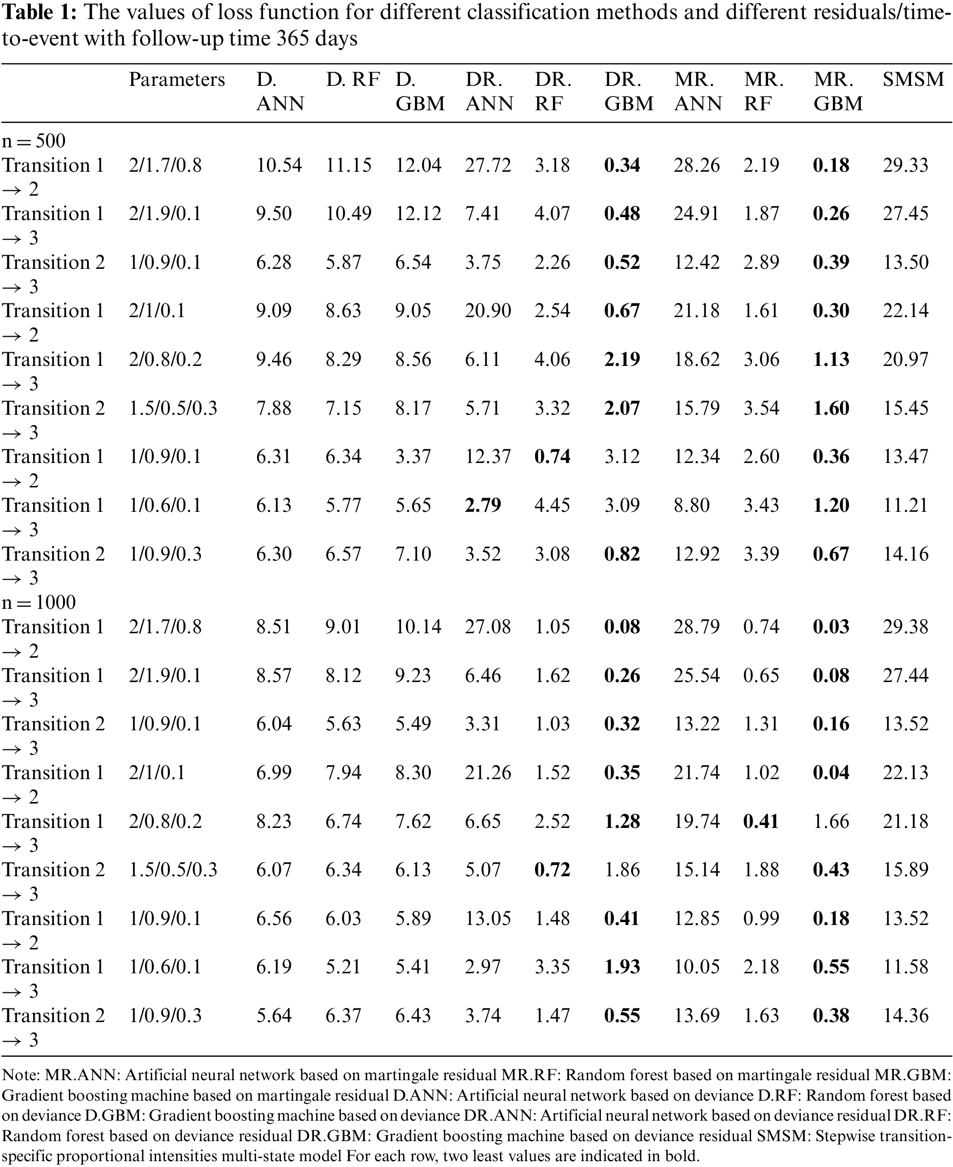
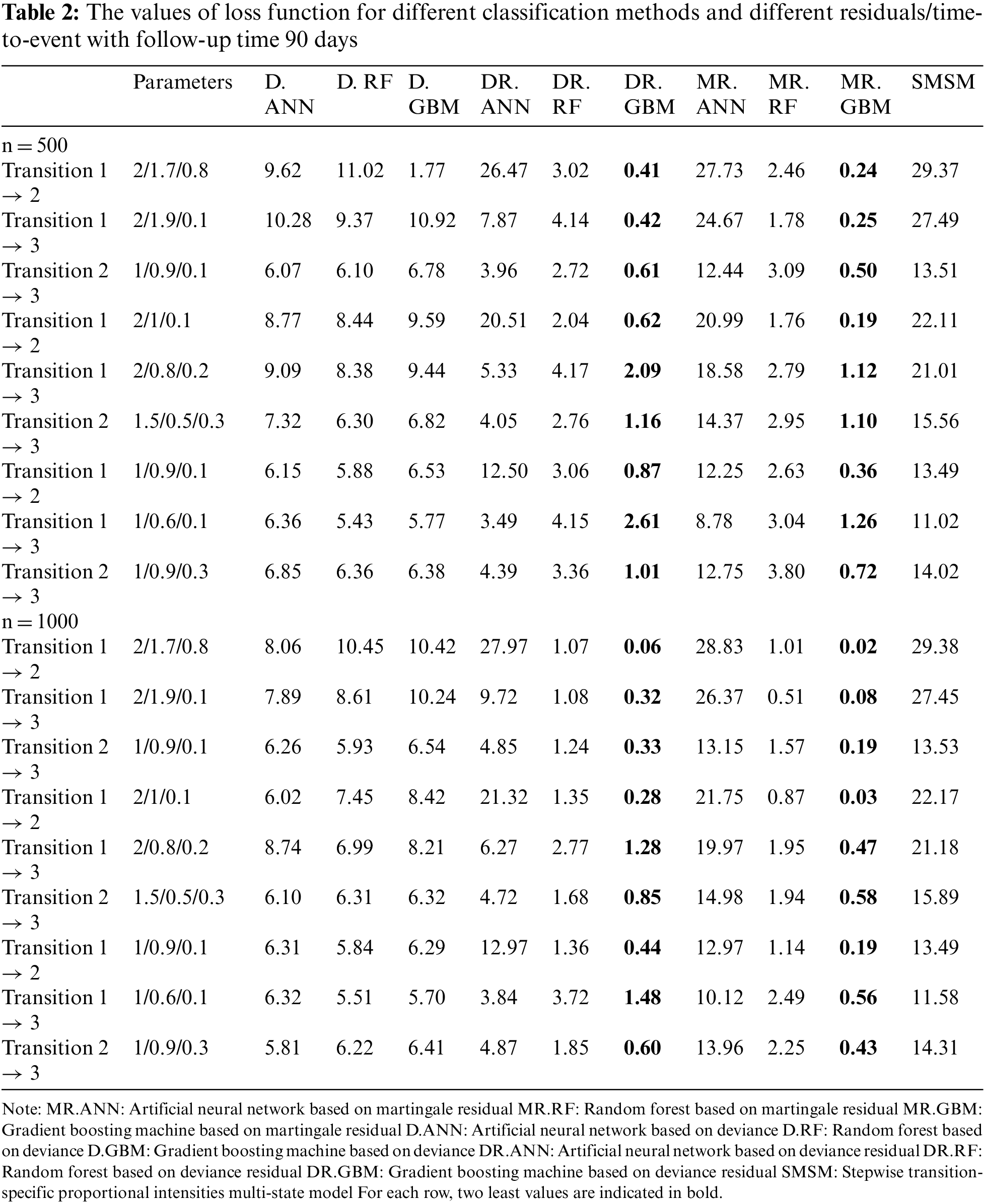
Tables 1 and 2 show the values of the loss function provided by different methods. Table 1 provides the results for a 1-year study, and Table 2 provides the results for a 3-month study. In these tables, the first column indicates the type of transition, the second column gives the values of the three effective parameters, and the subsequent columns give the mean value of the loss function provided by different methods. Columns 3 and 5 give the results for D, columns 6 and 8 show the results for DR, and columns 9 and 11 show the results for MR. As the simulation results show, the gradient boosting method on MR and DR provided the smallest loss values in almost all simulations for all transitions, respectively. The results also revealed that the proposed two-stage method has better performance for larger sample sizes. However, its performance was almost similar across different lengths of studies. The last column also shows the performance of the traditional multi-state model fitted to the generated data in simulations. According to the results, machine learning models outperformed the traditional model based on the Cox proportional hazards model.

4  Application

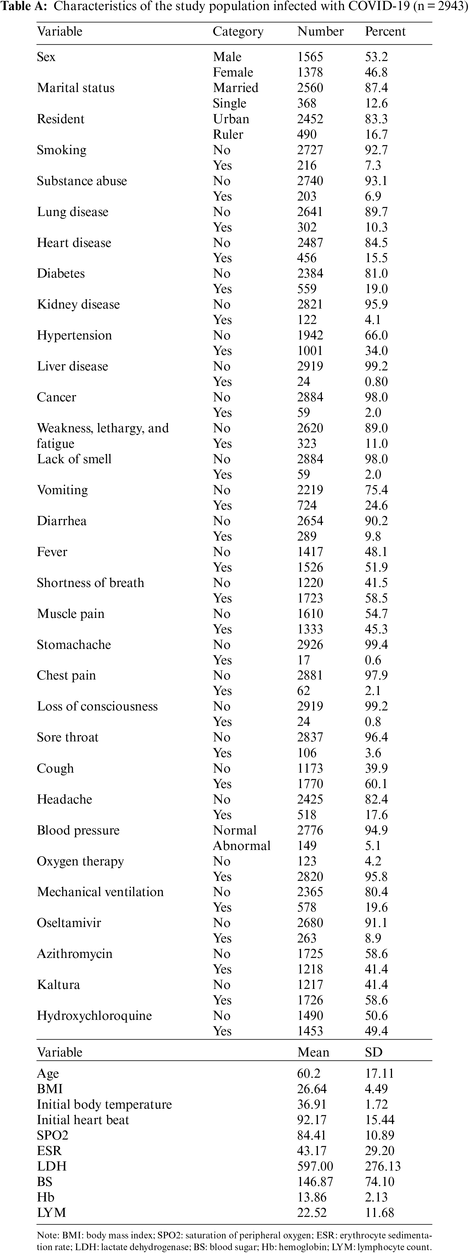
We apply our proposed two-step variable selection algorithm to a dataset of COVID-19 hospitalized patients. Each run took 30 s using an HP i5-laptop, RAM 8. The information of 2943 hospitalized patients with COVID-19 from February 20, 2020, to June 02, 2021 in Farshchian Medical Center and Shahid Beheshti Medical Center in Hamadan province, the west of Iran, was enrolled (Table A in the Appendix A). All of the patients were admitted to the ward (state 1). Then a patient may be transferred to the ICU (state 2) or die (state 3). The outcomes of interest were time to transfer to the ICU, time to death, and time to death after admission to the ICU. All patients who were alive at the end of the study were censored for death, and those who did not need to transfer to the ICU during the study were censored for admission to the ICU. The multi-state structure of the data is depicted in Fig. 1. The matrix below shows the number of observed transitions between different health states:

      1  2  3  Ω=123 (201685275043841400489)

This matrix gives the number of direct transitions between health states. In total, 852 patients were transferred to the ICU. A total of 489 patients died during the follow-up; among them, 414 patients died in the ICU and 75 patients died in the ward. In addition, 2454 patients were recovered and were considered as censored. Among them, a number of 2016 patients were censored for both transfer to ICU and death events, and a number of 438 patients were censored for death.

The mean (SD) and median age of patients were 60.2 (17.11) and 61.0 years, respectively. The clinical and demographic information of the patients are given in Appendix A. Here, we applied our proposed two-step algorithm to detect associated covariates with the risk of transition between different health states. We have used MR at the first step and gradient boosting at the second step. Figs. 2a–2c depicts the variable importance associated with Admission in ward → ICU, Admission in ward → Death, and ICU → Death, respectively. In this figure, the variables are ranked according to their importance. Based on Fig. 2a, the most important variables for the time from admission in the ward to transfer to the ICU were saturation of peripheral oxygen (SPO2), age, lymphocyte count (LYM), lactate dehydrogenase (LDH), hemoglobin (Hb), blood sugar (BS), initial heart rate, body mass index (BMI), erythrocyte sedimentation rate (ESR), and Oseltamivire, respectively. The most important variables for the transition from ward to death were age, SPO2, LYM, LDH, Hb, initial heart rate, ESR, heart disease, BMI, and cancer, respectively (Fig. 2b). Moreover, as given in Fig. 2c, SPO2, age, Hb, hydroxychloroquine, LDH, LYM, BS, ESR, initial heart rate, BMI, and Koltra were the most important variables at the time of transition from ICU to death. Among many others, these variables were chosen as the most important (presented in Appendix A ).

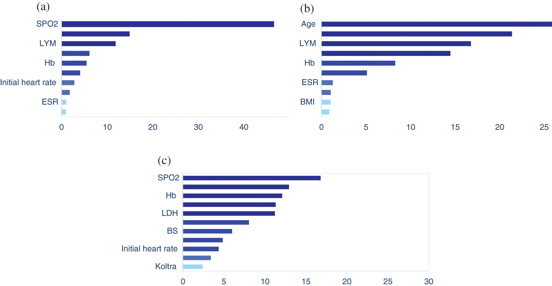
Figure 2: The results of variable importance based on martingale residual and gradient boosting algorithm for transitions from (a) Admission in ward to ICU, (b) Admission in ward to death, and (c) ICU to death, in hospitalized COVID-19 patients

Our case study revealed that SPO2 was an important predictor of the time of transition to the ICU and the time of death (among patients who were transferred to the ICU or not). Other studies have revealed that SPO2 affects the survival time and the length of hospital stay in COVID-19 patients [28]. According to Zhao et al. [29] a lower level of oxygen saturation at the time of admission is associated with a longer length of stay in the hospital.

Consistent with other studies, age was one of the most important predictors of the time of transition to ICU and the time of death among patients who were either transferred to ICU or not [28–31]. Several studies revealed that older patients were more likely to be transferred to the ICU and die [28,29]. Moreover, it has been shown that the age of the patients can influence the effects of other risk factors such as LYM on COVID-19 outcomes [32], which is an important risk factor for the disease progression [31,33]. These findings are consistent with the results of previous studies proposing that have shown that lower levels of LYM are related to the higher risk of admission to the ICU [32,34], such that ICU admitted patients had a decreased fraction of LYM compared to the other patients who were admitted to the ward [29]. Moreover, lower levels of LYM in peripheral blood were observed among patients who died [29].

The results also showed that the level of Hb is another important predictor for all three transitions, especially for mortality among ICU admitted patients. Other researchers have conducted different studies to evaluate the association between the severity of the disease or mortality and anemia among COVID-19 patients and they have received controversial results [30,35–39]. A meta-analysis study has shown that the levels of Hb were considerably lower than the normal level in patients with severe disease [40]. Several studies, mostly conducted in China, have shown an association between anemia and poor outcomes in hospitalized patients, and this may be because of its impact on immunity [38,39].

5  Discussions and Conclusions

Estimating variable importance in a multi-state process can be a challenging issue due to the complex relationships between variables. Classic variable selection methods like stepwise proportional hazards regression or penalized methods fail to provide an estimation of variable importance or considering complex/non-linear relationships between the inputs and outputs as well as the interaction between covariates. Therneau et al. [19] suggested that the martingale residual obtained from a null Cox model can be used as the outcome variable, so that usual regression analysis or classification methods like machine learning techniques can be applied to the new outcome variable (martingale residuals), and they provide very good results for survival data. This approach has also been applied for analyzing multivariate survival data like recurrent events. Nevertheless, few attempts have been made in relation to the multi-state data. In this paper, we proposed a two-step algorithm to evaluate the variable’s importance for MSMs. We applied neural network, random forest, and gradient boosting algorithms to the martingale residuals, deviance, and deviance residuals made from an MSM and compared their results. The simulation studies revealed that using gradient boosting on the martingale residuals and deviance residuals outperforms other algorithms. This may be due to the fact that the gradient boosting is trained sequentially, so that in the training process the errors in the previous steps are corrected. This is in contrast to methods like random forest, where the trees are parallel and are made independently. Gradient boosting is also able to capture complex patterns in the data. Moreover, the individual predictions, obtained from several independent trees (that are determined in any order) in the random forest, are aggregated (by the principal of the majority vote or the average value), while the sequence of gradient boosting does not change (it runs in a fixed order). Boosted trees are prone to overfitting and begin modeling the noise in the presence of noisy data, despite the benefits of gradient boosting.

In this study, we assumed a continuous and Markov multi-state process. Nevertheless, in other contexts, a semi-Markov or non-Markov process could be defined as well. In addition to considering ensemble methods, other model selection methods like support vector machines and deep learning methods can be introduced into the proposed residuals, which can be considered as a future work. Also, optimization of tuning parameters using heuristic algorithms like genetic algorithms or Bayesian optimization methods is worth investigating in future studies.

Here, we used our proposed method to identify the important variables at the time of transition from the ward to the ICU and death among COVID-19 patients who were admitted to the hospital. It should be noted that our goal in this case was simply to identify the most important variables influencing the risk of transitioning between different health states. To assess the direction and impact of the selected variables on the risk of different transitions, the use of classical multi-state models can be used as a complementary method. It is noteworthy that while there are too many studies that have utilized machine learning methods in COVID-19 data sets, no study has hybridized machine learning and multi-state methods, especially in analyzing COVID-19 data sets. This highlights the novelty aspect of this study.

Limitations

There were some limitations to the present study. In the data used in this study, information on only three states was available, including admission to the ward, ICU, and death. Although, there were patients who were retransferred to the ward from the ICU, their information was not available. So, our example had the illness-death multi-state structure. It is suggested to analyze more complex multi-state data sets with the provided model in this study. Another limitation was that dealing with time-dependent covariates is only possible by using martingale residual and adjusting martingale residual. Despite these limitations, the proposed method can be easily applied to the context of high-dimensional data like genome-wide association studies and medical image data to detect the most important genes or brain regions associated with survival outcomes more accurately than classic statistical methods.

Acknowledgement: We would like to appreciate the Vice-chancellor of Education of the Hamadan University of Medical Science for technical support for their approval and support of this work.

Ethics Approval and Consent to Participate: The data were collected from the patients’ medical recodes that have already been discharged and were not accessible for giving informed consent. A waiver of informed consent was awarded for the analysis conducted in this study by the Ethical Committee of the Hamadan University of Medical Sciences. All methods were carried out in accordance with relevant guidelines and regulations, and the study was approved by the Ethical Committee of the Hamadan University of Medical Sciences (IR.UMSHA.REC.1401.251; No. 140104072334).

Funding Statement: The authors received no specific funding for this study.

Conflicts of Interest: The authors declare that they have no conflicts of interest to report regarding the present study.

Appendix A. Characteristics of COVID-19 patients

References

1. Ferrer, L., Rondeau, V., Dignam, J., Pickles, T., Jacqmin-Gadda, H. et al. (2016). Joint modelling of longitudinal and multi-state processes: Application to clinical progressions in prostate cancer. Statistics in Medicine, 35(22), 3933–3948. DOI 10.1002/sim.6972. [Google Scholar] [CrossRef]
2. Mirzaee, M., Mohammad, K., Mahmoodi, M., Zeraati, H., Ebadzadeh, M. R. et al. (2014). Multi-state survival analysis in renal transplantation recipients. Iranian Journal of Public Health, 43(3), 316–322. [Google Scholar]
3. Ursino, M., Dupuis, C., Buetti, N., de Montmollin, E., Bouadma, L. et al. (2021). Multistate modeling of COVID-19 patients using a large multicentric prospective cohort of critically ill patients. Journal of Clinical Medicine, 10(3), 544. DOI 10.3390/jcm10030544. [Google Scholar] [CrossRef]
4. Beesley, L. J., Morgan, T. M., Spratt, D. E., Singhal, U., Feng, F. Y. et al. (2019). Individual and population comparisons of surgery and radiotherapy outcomes in prostate cancer using Bayesian multistate models. JAMA Network Open, 2(2), e187765. DOI 10.1001/jamanetworkopen.2018.7765. [Google Scholar] [CrossRef]
5. Dang, X., Huang, S., Qian, X. (2021). Risk factor identification in heterogeneous disease progression with L1-regularized multi-state models. Journal of Healthcare Informatics Research, 5(1), 20–53. DOI 10.1007/s41666-020-00085-1. [Google Scholar] [CrossRef]
6. Duan, R., Fu, H. (2015). Estimate variable importance for recurrent event outcomes with an application to identify hypoglycemia risk factors. Statistics in Medicine, 34(19), 2743–2754. DOI 10.1002/sim.6516. [Google Scholar] [CrossRef]
7. Sennhenn-Reulen, H., Kneib, T. (2016). Structured fusion lasso penalized multi-state models. Statistics in Medicine, 35(25), 4637–4659. DOI 10.1002/sim.7017. [Google Scholar] [CrossRef]
8. van der Laan, M. J. (2006). Statistical inference for variable importance. The International Journal of Biostatistics, 2(1), 1–31. DOI 10.2202/1557-4679.1008. [Google Scholar] [CrossRef]
9. Stachel, A., Daniel, K., Ding, D., Francois, F., Phillips, M. et al. (2021). Development and validation of a machine learning model to predict mortality risk in patients with COVID-19. BMJ Health & Care Informatics, 28(1), e100235. DOI 10.1136/bmjhci-2020-100235. [Google Scholar] [CrossRef]
10. Snider, B., McBean, E. A., Yawney, J., Gadsden, S. A., Patel, B. (2021). Identification of variable importance for predictions of mortality from COVID-19 using AI models for Ontario, Canada. Frontiers in Public Health, 9, 6757–6766. [Google Scholar]
11. Hazard, D., Kaier, K., von Cube, M., Grodd, M., Bugiera, L. et al. (2020). Joint analysis of duration of ventilation, length of intensive care, and mortality of COVID-19 patients: A multistate approach. BMC Medical Research Methodology, 20(1), 1–9. DOI 10.1186/s12874-020-01082-z. [Google Scholar] [CrossRef]
12. Breiman, L. (2001). Random forests. Machine Learning, 45(1), 5–32. DOI 10.1023/A:1010933404324. [Google Scholar] [CrossRef]
13. Breiman, L. (1996). Bagging predictors. Machine Learning, 24(2), 123–140. DOI 10.1007/BF00058655. [Google Scholar] [CrossRef]
14. Negassa, A., Ciampi, A., Abrahamowicz, M., Shapiro, S., Boivin, J. F. (2005). Tree-structured subgroup analysis for censored survival data: Validation of computationally inexpensive model selection criteria. Statistics and Computing, 15(3), 231–239. DOI 10.1007/s11222-005-1311-z. [Google Scholar] [CrossRef]
15. Andersen, P. K., Borgan, O., Gill, R. D., Keiding, N. (1993). Statistical models based on counting processes. New York: Springer-Verlag. [Google Scholar]
16. Andersen, P. K., Gill, R. D. (1982). Cox’s regression model for counting processes: A large sample study. The Annals of Statistics, 10(4), 1100–1120. DOI 10.1214/aos/1176345976. [Google Scholar] [CrossRef]
17. Cox, D. R. (1972). Regression models and life tables. Journal of the Royal Statistical Society: Series B (Methodological), 34(2), 187–202. [Google Scholar]
18. Cox, D. R. (1972). Breslow’s commons on regression models and life-tables. Journal of the Royal Statistical Society: Series B (Methodological), 23, 187–220. [Google Scholar]
19. Therneau, T. M., Grambsch, P. M., Fleming, T. R. (1990). Martingale-based residuals for survival models. Biometrika, 77(1), 147–160. DOI 10.1093/biomet/77.1.147. [Google Scholar] [CrossRef]
20. Natekin, A., Knoll, A. (2013). Gradient boosting machines, a tutorial. Frontiers in Neurorobotics, 7, 21. DOI 10.3389/fnbot.2013.00021. [Google Scholar] [CrossRef]
21. Freund, Y., Schapire, R. E. (1997). A decision-theoretic generalization of on-line learning and an application to boosting. Journal of Computer and System Sciences, 55(1), 119–139. DOI 10.1006/jcss.1997.1504. [Google Scholar] [CrossRef]
22. Friedman, J., Hastie, T., Tibshirani, R. (2000). Additive logistic regression: A statistical view of boosting (with discussion and a rejoinder by the authors). The Annals of Statistics, 28(2), 337–407. DOI 10.1214/aos/1016218223. [Google Scholar] [CrossRef]
23. Friedman, J. H. (2001). Greedy function approximation: A gradient boosting machine. Annals of Statistics, 29(5), 1189–1232. DOI 10.1214/aos/1013203451. [Google Scholar] [CrossRef]
24. Raj, P., Evangeline, P. (2020). The digital twin paradigm for smarter systems and environments: The industry use cases. London, UK: Academic Press. [Google Scholar]
25. Beyersmann, J., Allignol, A., Schumacher, M. (2012). Competing risks and multistate models with R. New York, NY: Springer Science & Business Media. [Google Scholar]
26. Crowther, M. J., Lambert, P. C. (2013). Simulating biologically plausible complex survival data. Statistics in Medicine, 32(23), 4118–4134. DOI 10.1002/sim.5823. [Google Scholar] [CrossRef]
27. Brent, R., Richard, P. (1973). Algorithms for minimization without derivatives. New York: Dover Publications. [Google Scholar]
28. Nasir, M., Perveen, R. A., Ahmad, S. N., Nazneen, R., Ahmed, S. M. P. (2021). Outcome of instrumental oxygen therapy in COVID-19: Survivors versus non-survivors in Bangladeshi cohort. American Journal of Internal Medicine, 9(1), 52–57. DOI 10.11648/j.ajim.20210901.18. [Google Scholar] [CrossRef]
29. Zhao, Z., Chen, A., Hou, W., Graham, J. M., Li, H. et al. (2020). Prediction model and risk scores of ICU admission and mortality in COVID-19. PLoS One, 15(7), e0236618. DOI 10.1371/journal.pone.0236618. [Google Scholar] [CrossRef]
30. Guan, W. J., Ni, Z. Y., Hu, Y., Liang, W. H., Ou, C. Q. et al. (2020). Clinical characteristics of coronavirus disease 2019 in China. New England Journal of Medicine, 382(18), 1708–1720. DOI 10.1056/NEJMoa2002032. [Google Scholar] [CrossRef]
31. Lu, J., Hu, S., Fan, R., Liu, Z., Yin, X. et al. (2020). ACP risk grade: A simple mortality index for patients with confirmed or suspected severe acute respiratory syndrome coronavirus 2 disease (COVID-19) during the early stage of outbreak in Wuhan, China. DOI 10.1101/2020.02.20.20025510. [Google Scholar] [CrossRef]
32. Huang, C., Wang, Y., Li, X., Ren, L., Zhao, J. et al. (2020). Clinical features of patients infected with 2019 novel coronavirus in Wuhan, China. The Lancet, 395(10223), 497–506. DOI 10.1016/S0140-6736(20)30183-5. [Google Scholar] [CrossRef]
33. Hou, W., Zhang, W., Jin, R., Liang, L., Xu, B. et al. (2020). Risk factors for disease progression in hospitalized patients with COVID-19: A retrospective cohort study. Infectious Diseases, 52(7), 498–505. DOI 10.1080/23744235.2020.1759817. [Google Scholar] [CrossRef]
34. Ng, D. H., Choy, C. Y., Chan, Y. H., Young, B. E., Fong, S. W. et al. (2020). Fever patterns, cytokine profiles, and outcomes in COVID-19. Open Forum Infectious Diseases, 7(9), ofaa375. DOI 10.1093/ofid/ofaa375. [Google Scholar] [CrossRef]
35. Bellmann-Weiler, R., Lanser, L., Barket, R., Rangger, L., Schapfl, A. et al. (2020). Prevalence and predictive value of anemia and dysregulated iron homeostasis in patients with COVID-19 infection. Journal of Clinical Medicine, 9(8), 2429. DOI 10.3390/jcm9082429. [Google Scholar] [CrossRef]
36. Tao, Z., Xu, J., Chen, W., Yang, Z., Xu, X. et al. (2021). Anemia is associated with severe illness in COVID-19: A retrospective cohort study. Journal of Medical Virology, 93(3), 1478–1488. DOI 10.1002/jmv.26444. [Google Scholar] [CrossRef]
37. Young, B. E., Ong, S. W. X., Kalimuddin, S., Low, J. G., Tan, S. Y. et al. (2020). Epidemiologic features and clinical course of patients infected with SARS-CoV-2 in Singapore. JAMA, 323(15), 1488–1494. DOI 10.1001/jama.2020.3204. [Google Scholar] [CrossRef]
38. Ryan, A. S. (1997). Iron-deficiency anemia in infant development: Implications for growth, cognitive development, resistance to infection, and iron supplementation. American Journal of Biological Anthropology, 104(S25), 25–62. DOI 10.1002/(ISSN)1096-8644. [Google Scholar] [CrossRef]
39. Dinevari, M. F., Somi, M. H., Majd, E. S., Farhangi, M. A., Nikniaz, Z. (2021). Anemia predicts poor outcomes of COVID-19 in hospitalized patients: A prospective study in Iran. BMC Infectious Diseases, 21(1), 1–7. [Google Scholar]
40. Lippi, G., Mattiuzzi, C. (2020). Hemoglobin value may be decreased in patients with severe coronavirus disease 2019. Hematology, Transfusion and Cell Therapy, 42, 116–117. [Google Scholar]