
 Submit a Paper
 Propose a Special lssue
 Open Access
ARTICLE

New Perspective to Isogeometric Analysis: Solving Isogeometric Analysis Problem by Fitting Load Function
1
School of Mathematical Sciences, Zhejiang University, Hangzhou, 310058, China
2
State Key Lab. of CAD&CG, Zhejiang University, Hangzhou, 310058, China
* Corresponding Author: Hongwei Lin. Email:
(This article belongs to the Special Issue: Integration of Geometric Modeling and Numerical Simulation)
Computer Modeling in Engineering & Sciences 2023, 136(3), 2957-2984. https://doi.org/10.32604/cmes.2023.025983
Received 08 August 2022; Accepted 20 October 2022; Issue published 09 March 2023
 View Full Text
 Download PDF
Abstract
Isogeometric analysis (IGA) is introduced to establish the direct link between computer-aided design and analysis. It is commonly implemented by Galerkin formulations (isogeometric Galerkin, IGA-G) through the use of nonuniform rational B-splines (NURBS) basis functions for geometric design and analysis. Another promising approach, isogeometric collocation (IGA-C), working directly with the strong form of the partial differential equation (PDE) over the physical domain defined by NURBS geometry, calculates the derivatives of the numerical solution at the chosen collocation points. In a typical IGA, the knot vector of the NURBS numerical solution is only determined by the physical domain. A new perspective on the IGA method is proposed in this study to improve the accuracy and convergence of the solution. Solving the PDE with IGA can be regarded as fitting the load function defined on the NURBS geometry (right-hand side) with derivatives of the NURBS numerical solution (left-hand side). Moreover, the design of the knot vector has a close relationship to the NURBS functions to be fitted in the area of data fitting in geometric design. Therefore, the detected feature points of the load function are integrated into the initial knot vector of the physical domain to construct the new knot vector of the numerical solution. Then, they are connected seamlessly with the IGA-C framework for its great potential combining the accuracy and smoothness merits with the computational efficiency, which we call isogeometric collocation by fitting load function (IGA-CL). In numerical experiments, we implement our method to solve 1D, 2D, and 3D PDEs and demonstrate the improvement in accuracy by comparing it with the standard IGA-C method. We also verify the superiority in the accuracy of our knot selection scheme when employed in the IGA-G method, which we call isogeometric Galerkin by fitting load function (IGA-GL).Graphic Abstract
Keywords
Isogeometric analysis (IGA) [1] is a computational mechanics technology that advances the seamless integration between computer-aided design (CAD) and computer-aided engineering (CAE). Although finite element analysis (FEA) [2] gains widespread applications in physical simulation, IGA uses the same nonuniform rational B-spline (NURBS) bases [3] as the physical domain space to construct the numerical solution domain space. Based on these NURBS basis functions, IGA can directly deal with the NURBS-based CAD model. This condition avoids tedious and time-consuming mesh generation in classical FEA when CAD model simulation is performed. Therefore, IGA saves a considerable amount of computation and greatly improves the numerical accuracy of the solution.
IGA has been initially implemented by Galerkin formulations (isogeometric Galerkin (IGA-G)) [1], thereby raising the efficiency issue due to the numerical integration. Isogeometric collocation (IGA-C) [4] focuses on solving the strong form of partial differential equations (PDEs) [5] rather than the weak form in IGA-G to promote the accuracy-to-computational-cost ratio. Substituting the derivatives of the NURBS numerical solution at some collocation points into the PDE leads to a linear system. The selection of these collocation points is the key to accuracy and convergence rate.
When PDEs are solved over a physical domain defined by a NURBS geometry, typical IGA commonly takes the NURBS as the bases of the approximation solution space, which is the same as the NURBS bases that construct the physical domain space. The NURBS bases are determined totally by the knot vector [3]. This fact indicates that the knot vectors for the NURBS bases of the solution field are directly inherited from the knot vectors of the geometry representation. However, few previous works investigated the influence of the knot vector on the approximating accuracy and convergence rate of the numerical solution. On the other hand, in the area of the data fitting in geometric design, the feature points that depict the shape and characteristics of the NURBS function to be fitted are vital to the knot vector that constructs the NURBS bases [3,6,7]. A theorem stating that the spline numerical solution and its k-order derivative have the same breakpoint sequence has been proposed and proved in [8]. Thus, we can treat the left-hand side and right-hand side of the PDE as a fitting problem, that is, approximating the load function defined by the NURBS geometry (right-hand side) with the derivatives of the NURBS numerical solution (left-hand side).
A new method of IGA is proposed in this study to improve the accuracy when PDEs are solved over the physical domain defined by NURBS geometry. We exploit the idea that the knot vector of the NURBS numerical solution is decided together by the load function and geometry representation. The feature points of the load function over the physical domain are detected in 1D, 2D, and 3D cases. Then, we merge these feature points into the initial knot vector of the spline representation of the physical domain. Given the great potential of the computational efficiency of IGA-C, we focus on the performance of the IGA-C framework with our generated knot vector. Thus, we name it as IGA-C by fitting load function (IGA-CL) method. In numerical experiments, we implement our IGA-CL framework to solve 1D, 2D, and 3D PDEs at Greville abscissae [4] and superconvergent (SC) collocation [9]. We demonstrate the efficiency of our method in terms of numerical accuracy in analysis by comparing it with the typical IGA-C method, where the knot vector of the numerical solution is the same as the knot vector of the physical domain. We also show the superiority of the knot selection scheme applied in the IGA-G framework over the typical IGA-G, which we call IGA-G by fitting load function (IGA-GL).
The rest of this paper is structured as follows: Section 1.1 provides the related work. The preliminary of the IGA is provided in Section 2. We present an overview of our IGA-CL framework in Section 3. Section 4 presents the strategy to detect feature points of load functions of the PDEs in 1D, 2D, and 3D cases. Section 4.4 introduces the method to generate the integrated knot vectors and proposes our IGA-CL framework. Section 5 conducts experiments for solving PDEs in 1D, 2D, and 3D cases and applying the IGA-G method. The comparisons exhibit the influences of numerical accuracy in terms of our knot selection. Finally, the conclusions and perspectives on future works are detailed in Section 6.
IGA-G and applications. IGA was first introduced by [1] in 2005 to bridge the gap between CAD and CAE. The core idea of IGA is to utilize the same smooth and high-order NURBS bases for both the geometry parameterization and solution approximation. The finite element method (FEM) [2] in analysis has grown strong sufficiently. However, FEM always suffers from the time-consuming mesh generation and mesh approximation error. IGA possesses some additional merits over the traditional FEM [1,10], such as high continuity, exact representation of geometry, and low computational cost, because IGA directly takes the NURBS-expressed physical domain as the computational domain and computes on the control mesh.
The standard IGA method is implemented by Galerkin formulation (IGA-G) based on the weak form of the problem. The stiffness matrix assembly involves many numerical integrations, such as the commonly used Gauss quadrature. The integration efficiency in IGA has been first considered by [11]. Then, Gauss-Galerkin quadrature rules [12] and optimal and reduced quadrature rules [13] were developed. A promising approach for reusing the basis function evaluations in the numerical integration has been recently presented to improve the accuracy and time cost in [14]. In addition to tensor product B-splines, the isogeometric Galerkin matrices with hierarchical B-splines were efficiently computed through the interpolation, look-up and sum factorization techniques [15,16]. In the past 20 years, IGA has been widely applied in physical simulations such as structural mechanics [17–19], fluid mechanics [20–22], elastic mechanics [23–25], and shape optimization problems [26–28]. Its overview and computer implementation aspects were presented by [29].
IGA-C and applications. Although the mainstream IGA-G method based on the discretization of the weak form has the optimal convergence of
The research of IGA-C is mostly limited by the options of the ideal collocation points. In IGA-C, the commonly used collocation points are Greville abscissae [4] and Demko abscissae [30,32]. Demko abscissae are obtained from the extreme points of Chebyshev splines, and Greville abscissae are acquired from the averaging operation of the knot vector. However, their convergence orders are
Data point sampling and fitting. In geometric design, the quality of curve/surface fitting is related to the quality of data point sampling. Efficient sampling methods enable the reconstruction of a curve/surface with a limited amount of points [43]. Filip et al. [44] estimated the number of isometric parameter points using the bounds on derivatives. Park [45] utilized an offset envelope of a line segment and presented the approximation of error-bounded polygons. This approximation plays an important role in Hausdorff distance between the control segments and the corresponding curves. Razdan [46] discussed the uniform sampling of arc length or total curvature. Then an iteration algorithm was proposed to sample arc length or weighted arc length uniformly and the bending energy [47]. Pagani et al. [43] have acquired certain sampled points in terms of the mean of the arc length and total curvature. The reconstruction of the curve and surface outperforms the uniform sampling method. Instead of the uniform sampling method, Lu et al. [48] focused on the sampling feature points on planar parameter curves to retain the shapes of the original curves and weigh the arc length and the total curvature to sample points. This method is different from uniform sampling but closely related to the feature points.
2.1 Isogeometric Galerkin Method
In CAD, the physical domain is expressed by a NURBS mapping from a parametric domain
where
We name
where
In particular, let the following Laplace equation over the physical domain defined by a NURBS geometry
where the Dirichlet boundary
The IGA-G method ([1]) focuses on the weak form of the PDE, which is given by
where the weighting function
Galerkin’s method aims to construct the finite-dimensional approximations of the spaces
Then the weak form can be transformed into
By assembling the system of the weak form (7), we finally solve the following linear equations and obtain the solution
2.2 Isogeometric Collocation Method
The IGA-C method ([4]) is also proposed to solve the PDE. In general, the boundary value problem (BVP) can be summarized as follows:
where
IGA-C solves the equations by introducing a set of collocation points
When
The IGA-G and IGA-C methods involve the derivatives of the NURBS basis functions when the numerical solution

Figure 1: The cubic NURBS basis
Therefore, the feature points on the load function f(x) are essential to the knot vector for the left-hand-side fitted function and for the numerical solution
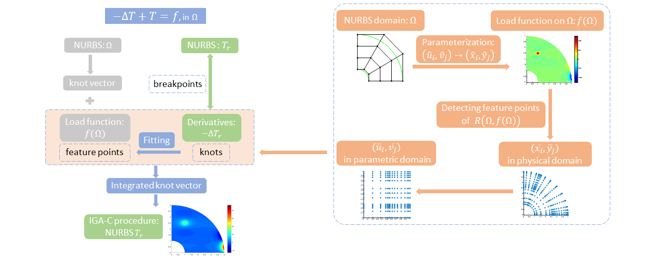
Given the great potential of computational efficiency of IGA-C, this study focuses on the performance of IGA-C framework with our generated knot vector. We propose the IGA-CL method, which combines the representation of the physical domain and the load function characteristics to construct the knot vector for the numerical solution in the IGA-C framework. The main idea is illustrated in Fig. 2. First, uniform parameterization of the physical domain defined by the NURBS geometry is done in the parametric domain to obtain a set of parameters, and the corresponding coordinates in the physical domain are calculated by NURBS mapping. Second, via feature point detection operation of the load function presented in Section 4, we choose the parameters assigned to these feature points, which serve as the knots to insert into the initial knot vector for the physical domain. Finally, on the basis of the integrated knot vector, we construct the NURBS bases for the numerical solution that are different from the initial bases for the physical domain. We employ the IGA-C framework to obtain the numerical solution to the BVP, where both the basis functions and collocation points depend on our integrated knot vector.

Figure 2: The main idea of IGA-CL: The integrated knot vector combines the initial knot vector of the physical domain
4 Generation of Knot Vectors by Detecting Feature Points of Load Functions
In this section, we introduce the detecting method of feature points from the load functions of the PDEs defined on a physical domain represented by NURBS geometry. We develop a method of knot generation to construct the knot vector once the feature points are detected.
We begin with the detecting method of the load function of the PDE in a 1D case. Comparing with uniform sampling methods using arc length and curvature information ([43,47]), Lu et al. [48] devised a nonuniform point sampling method for fitting the parametric curves with B-spline curves. This method captures the salient features on the curve and produces noticeable fitting results. It begins with the uniform parameterization of the parametric curve; thus, we employ the uniform parameterization to our NURBS-expressed physical domain. Therefore, we obtain the coordinates in the physical domain by NURBS mapping corresponding to the generated parameters and the load function values at these coordinates. Suppose the load function
and
First, the physical domain
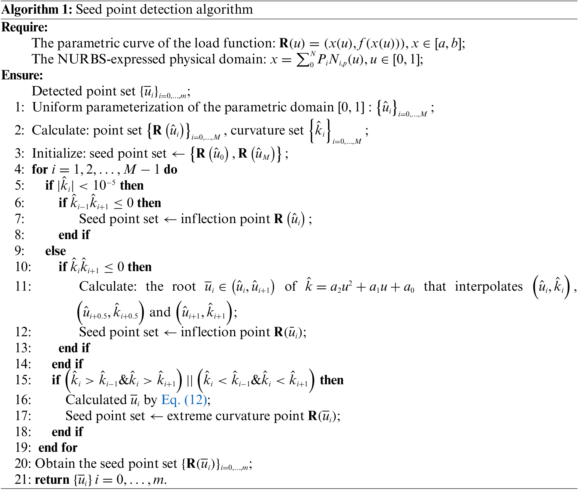
The seed points include endpoints, inflection points, and extreme curvature points, which are determined by referring to [48]. In the present study, we briefly summarize the rules of determination as follows:
Inflection points If
Extreme curvature points If the conditions of
Then
The seed point detection is concluded in Algorithm 1. As illustrated, the domain [0, 1] of the parametric curve of the load function
:
The seed point set
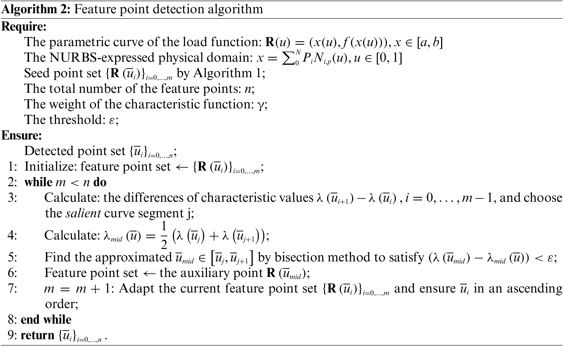
Define
where
Apparently,
The feature point detection is presented in Algorithm 2. Algorithm 1 returns
2D case is regarded as the extension of the 1D case along the
A load function f(x, y) with parametric surface is written as
where
The mean curvature of the two principle curvatures is good for reflecting the surface shape. Nevertheless, we maintain the curvature computed in each direction without loss of generality. Fix
The curvature of the load function f at point
Subsequently, we express the marginal cumulative integrals of curvature along the u- and v-directions:
Thus, the marginal cumulative characteristic functions along the u- and v-directions are constructed as follows:
Based on
:
4.3 Three-Dimensional Detection
For the 3D case, we construct the characteristic functions in a way similar to that in the 2D case. The load function is f(x, y, z) and the parametric solid is
where
The volume of the parametric solid is presented as below:
Thus, the marginal cumulative volumes in three directions can be described as
On the other hand, the curvatures in
Then, the curvature of the load function f at point
The marginal cumulative integrals of the curvature in u-, v-, and w-directions are
Therefore, the marginal cumulative characteristic functions of the load function f in three directions are constructed as follows:
Given that the process is similar to surface detection, we omit the details here.
Many numerical approaches were proposed to solve PDEs, among which IGA-C is an efficient method, which is described in Section 2.2. However, the knot vector of the IGA-C method can influence not only the NURBS bases for the numerical solution but also the collocation points.
Given the 1D scenario, the other two cases are treated similarly. Since the point detection is done, we obtain the feature point set
we generate additional knots by averaging operation ([3]) based on Schoenberg-Whitney theorem ([49]) from the feature points for each direction in curve/surface fitting:
Moreover, Hosseini et al. summarized three knot placement techniques for geometric construction from the data points to decide the positions of the internal knots of the knot vector ([50]), namely, uniform knot placement, De Boor’s algorithm, and Piegl and Tiller’s algorithm. Here, the generated knots representing the characteristics of the load function are inserted into the knot vector U. The knots
The spline numerical solution is then expressed as
Employing collocation schemes such as Greville abscissae, superconvergent points, and Cauchy-Galerkin points yields a set of collocation points. Replacing the unknown function T(u) in the PDE with the numerical solution
In this section, we validate the influence of computing accuracy with our isogeometric analysis by fitting load functions in solving PDEs through numerical experiments. The typical IGA-C and our IGA-CL are compared in Sections 5.1–5.3. We verify that the IGA-CL method outperforms IGA-C by contrasting relative errors and absolute errors, particularly for the case when the solution has obvious characteristics. In addition, we extend to exploit the IGA-GL method, which displays the same superiority of the accuracy over the typical IGA-G method through the comparisons in Section 5.4. For the following examples, relative error
where t stands for the transpose, the analytical solution and numerical solution are denoted as T and
Example I: A 1D Poisson problem with Dirichlet boundary condition:
where
and the analytical solution is
Given the advantage of our IGA-CL method, we utilize the feature points of the load function and construct an integrated knot vector. To verify the accuracy improvement, we apply our IGA-CL framework to solve Eq. (31) and compare it with the typical IGA-C at Greville abscissae ([4]) and other collocation schemes such as SC points ([9]) of the same degrees of freedom.
Fig. 3a displays the detecting points of the load function

Figure 3: Our detected points on the load function and the corresponding cubic NURBS bases with knot generation method
Fig. 4 shows the comparisons of convergence of the relative error by exploiting our IGA-CL framework and the typical IGA-C framework at Greville abscissae with the same degrees of freedom under different degrees of the bases. The convergence of solving this 1D problem by IGA-CL with the integrated knot vector is expressed by solid lines, whereas the convergence by typical IGA-C is displayed by dashed lines. We denote the abscissa as

Figure 4: Convergence comparison of IGA-CL/IGA-C at Greville collocation points under different degrees of Example I
Let the ordinate be the
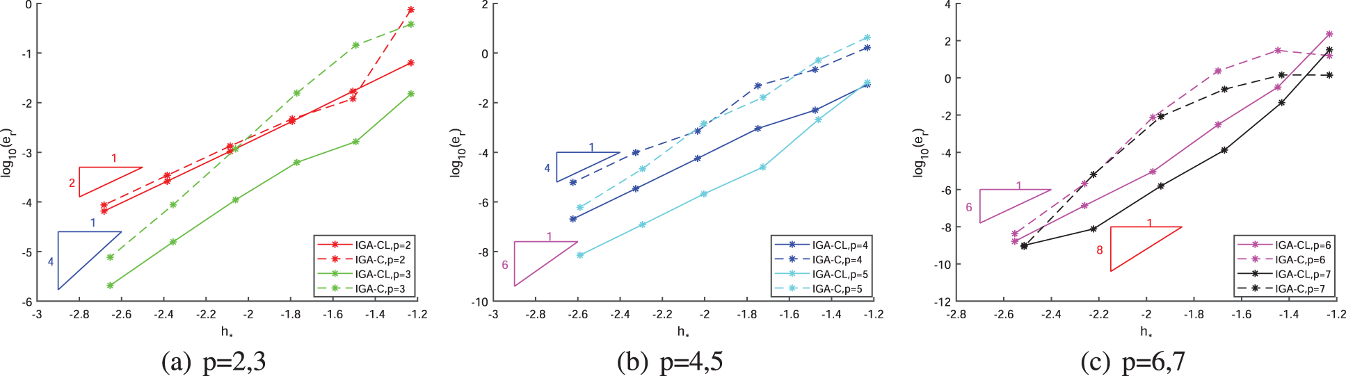
Figure 5: Convergence comparison of IGA-CL/IGA-C at SC points under different degrees of Example I
Our method demonstrates its superiority over typical IGA-C in terms of accuracy under all the degrees p of the NURBS basis functions. Because of the knot selection from the load function, the relative errors of small dofs at the beginning of IGA-CL are much lower than those of the typical IGA-C that uses the knot vector only from the physical domain. The general convergence rates of IGA-CL remain unchanged or slightly lower than those of IGA-C. For Greville collocation points, the convergence orders of IGA-C and IGA-CL are both
For PDEs under other boundary conditions, we present the following example:
Example II: A 1D ODE with Dirichlet and Neumann boundary conditions:
where
and the analytical solution is
In this case, we set the parameter
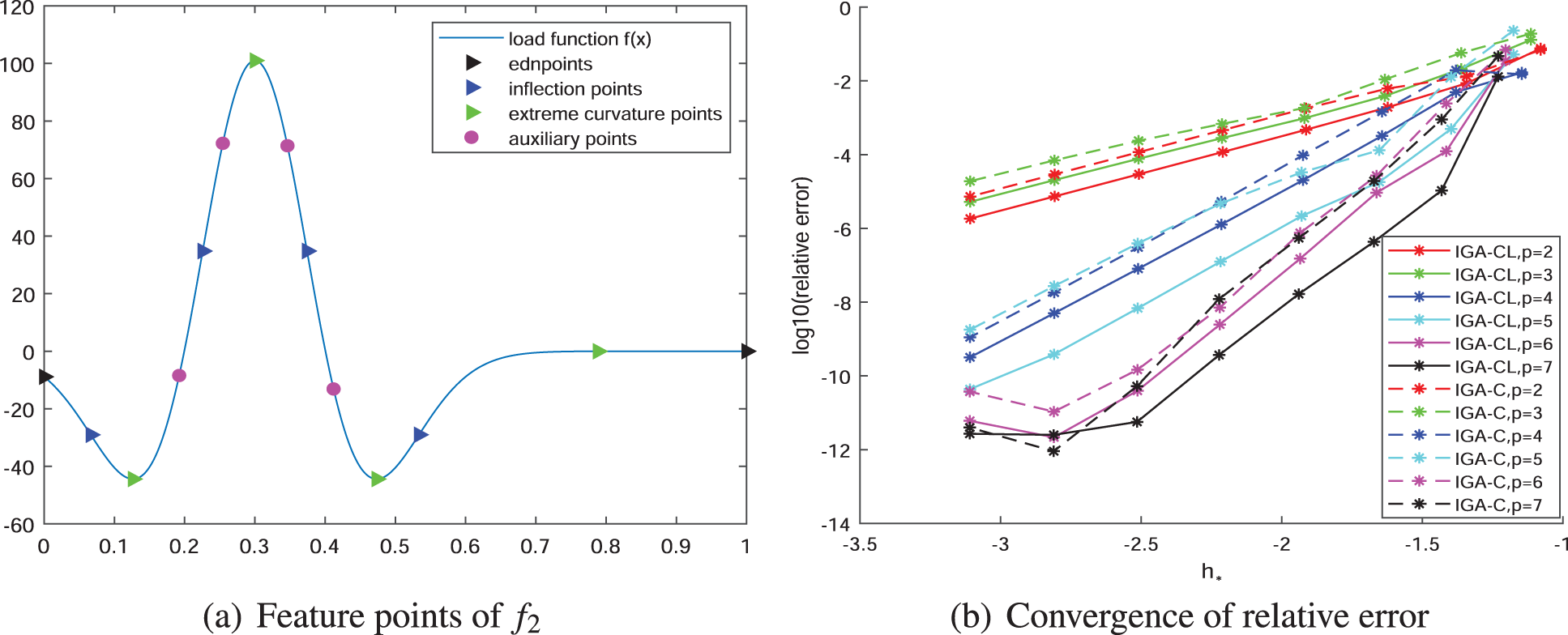
Figure 6: Detected points on the load function and the convergence results of relative error
We compare IGA-CL with IGA-C at Greville abscissae and SC points in solving the following two 2D Examples III and IV. The main idea of the IGA-CL is detecting the feature points on the load function and then linking them to IGA-C for solving PDEs. Whether the accuracy of the IGA-CL solution outperforms IGA-C principally depends on the quality of the feature points detected. The weights in the characteristic functions can be controlled and adjusted, thereby influencing the detection effect. We show the convergence of examples with a relatively satisfying choice of weight.
Example III: A 2D Poisson problem on a quarter of an annulus
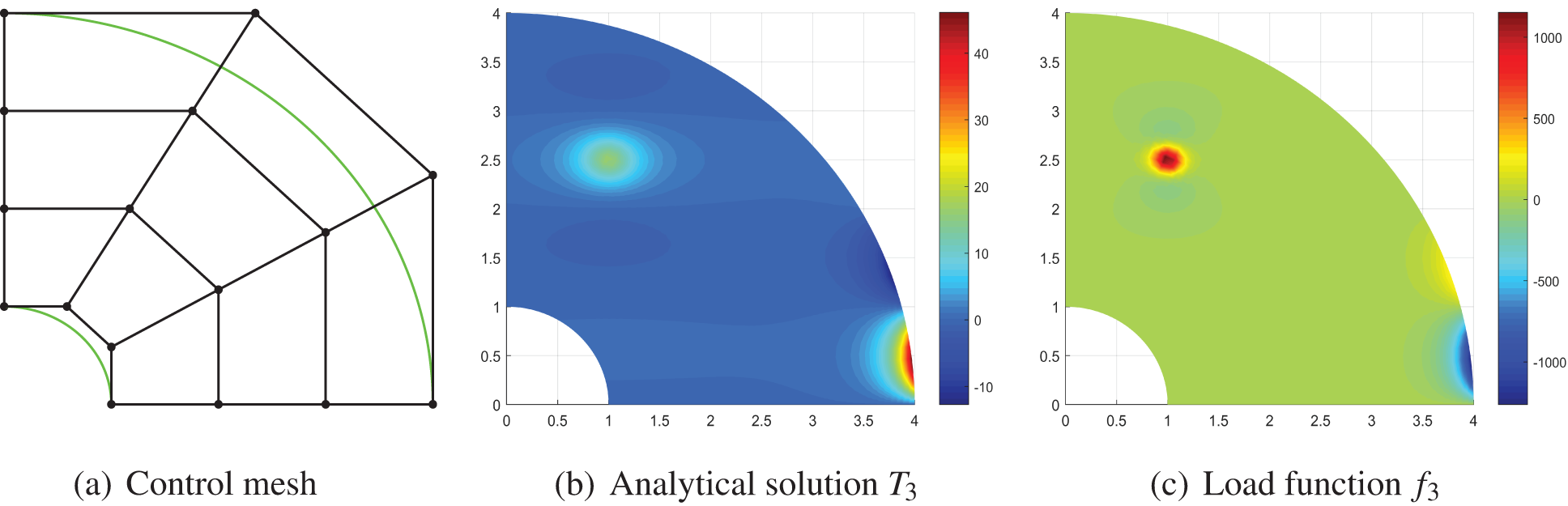
Figure 7: Example III. The analytical solution and the load function have nearly the same characteristics
The load function is
where
Example IV: An elliptic PDE on a quarter of a plate with a circular hole
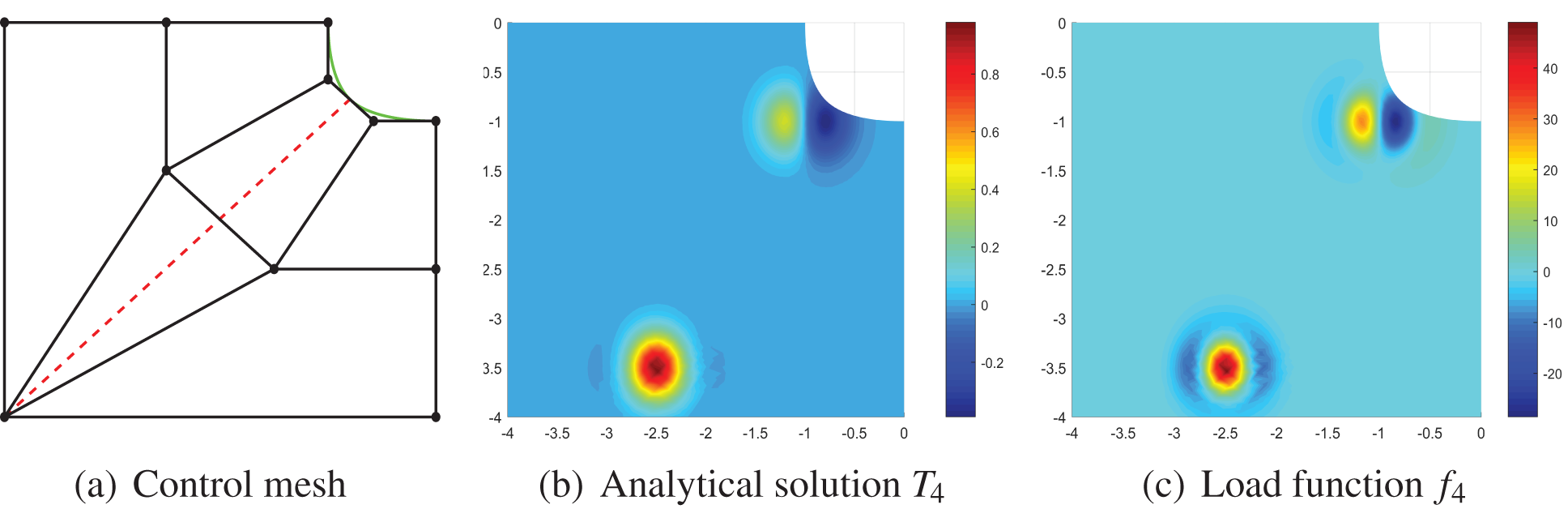
Figure 8: Example IV. The analytical solution and the load function have nearly the same characteristics
The load function is
where
To begin with, we present Figs. 7 and 8 displaying the analytical solutions and the load functions to demonstrate the effectiveness of our method. For the convenience of comparing errors, the analytical solutions for all experiments in this study are assumed to be known. In fact, in “real settings”, the “exact” solutions could be computed with a dense mesh. It is observed that the load functions roughly retain the characteristics of the analytical solutions of the PDEs. Consequently, detecting the feature points of the load function is a helpful guidance when solving PDEs.
In order to solve the elliptic equations Examples III and IV, the IGA-CL and IGA-C methods at Greville and SC collocation points are employed and compared in terms of absolute error. The initial number of detected points is
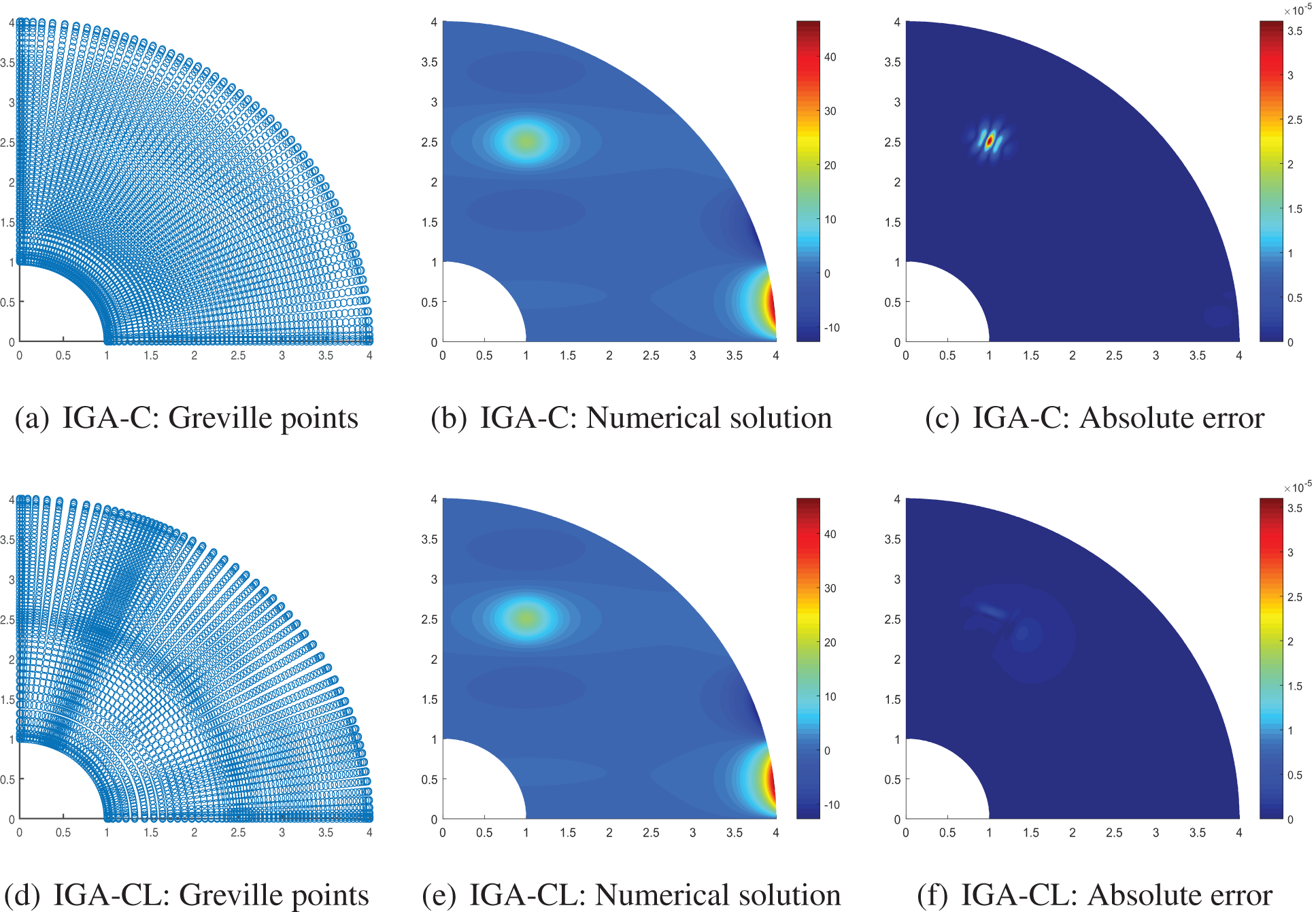
Figure 9: Comparison of IGA-CL/IGA-C solution of Example III after three times of h-refinement

Figure 10: Comparison of IGA-CL/IGA-C solution of Example IV after three times of h-refinement
However, in these two cases, considering the extreme nonuniformity after h-refinements when a small weight is adopted, we take a large weight in practical experiments to ensure that the flat part of the shape of load function has fairly and evenly detected points. For simplicity, the weights we adopted here are
Figs. 9d and 10d show that the distribution of the collocation points in the physical domain is very related to the solution. This finding indicates that the initial number of the detected points adopted in the area where the load function reaches the local maximum or the minimum is more than the number of detected points in the area where the load function appears steady. Through the comparisons of absolute error between IGA-C and IGA-CL methods, our IGA-CL method has a much lower error than IGA-C method.
With the appropriate weights, we exhibit the convergence comparisons of the relative error of IGA-CL and IGA-C at Greville abscissae and SC points under different degrees of NURBS bases of the numerical solution of Examples III and IV in Figs. 11 and 12, respectively. Our IGA-CL outperforms IGA-C distinctly under the same dofs. The convergence orders of the IGA-CL solution appear a little lower than those of IGA-C because the difference between the size of knot intervals of IGA-C and IGA-CL diminishes as the dofs increase. However, IGA-CL solutions still show an obvious increase in accuracy, which is conspicuously considerable.
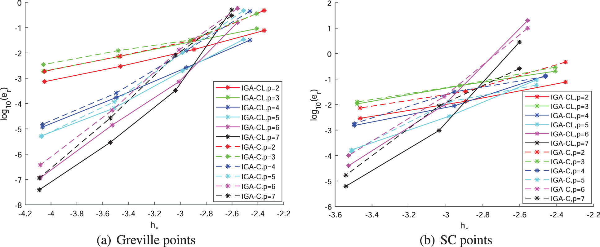
Figure 11: Convergence comparison of IGA-CL/IGA-C at Greville/SC collocation under different degrees of Example III

Figure 12: Convergence comparison of IGA-CL/IGA-C at Greville/SC collocation under different degrees of Example IV
Example V: A 3D elliptic PDE, on a unit cube with Dirichlet boundary condition is given as follows:
where
and the analytical solution is
In this case, the initial number of feature points that we sampled in our IGA-CL method is 6 for each direction, and the weights in characteristic functions are
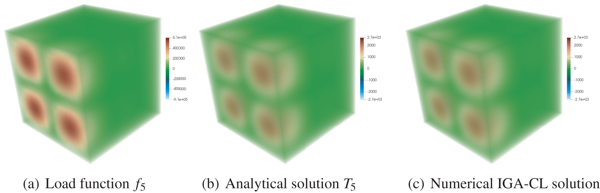
Figure 13: IGA-CL solution of Example V after two times of h-refinements
Then, we compare the distribution of absolute errors between IGA-CL and IGA-C at Greville abscissae with the same dofs at an arbitrary degree of the numerical solution after two times of h-refinements, as shown in Fig. 14. The absolute errors of IGA-CL and IGA-C methods are shown when
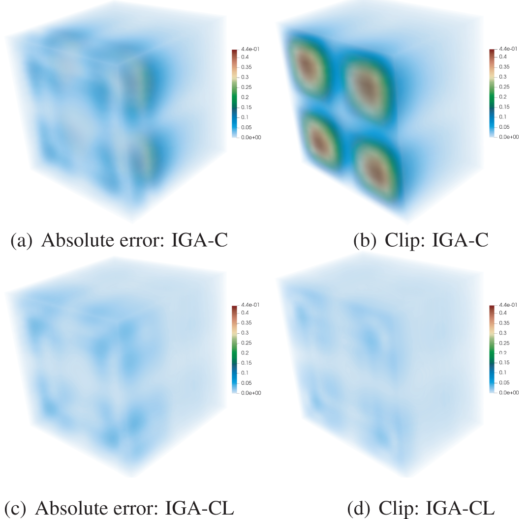
Figure 14: The absolute errors of IGA-CL/IGA-C at Greville abscissae of Example V. The second column is the clip view of the first column. The maximum absolute errors of IGA-C and IGA-CL methods are 0.4390 and 0.0775, respectively
The convergence figures of relative errors are also shown. Fig. 15 presents the comparison of the convergence of relative error between IGA-CL and IGA-C under different degrees of the bases of the numerical solution. Except that the convergence curves of the two methods coincide when the degrees are
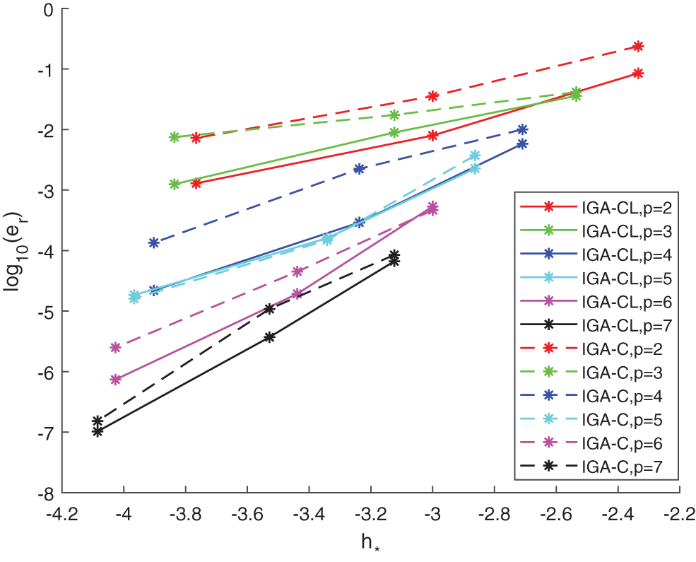
Figure 15: Convergence comparison of IGA-CL/IGA-C at Greville collocation under different degrees of Example V
One concern that should be addressed is that the detection of the feature points as a pre-processing costs time. Here we show the comparison of the time cost and relative error between IGA-CL and IGA-C in Table 1. The detection of feature points includes two parts: the calculation of curvatures of the sampling points, and the detection using characteristic function. The computation realizes the IGA framework to solve PDEs. We implemented them with MATLAB on an 8G laptop. From the table, we observe that the computation time of IGA-CL and IGA-C is almost the same due to the same framework, while IGA-CL has additional time cost of pre-processing on detection of feature points. Although there is a little extra time for feature point detection in IGA-CL, the precision of IGA-CL is higher than that of IGA-C.

Based on the knot selection scheme, IGA concentrating on load function is applicable not only to the IGA-C method, but also to the IGA-G method. For Example I in Section 5.1, Fig. 16 also shows the superiority of our knot generation by fitting the load function in the IGA-G method over the typical IGA-G method. Since we employ the integrated knot vector to the IGA-G, we call the improved method as IGA-GL. From the initial degrees of freedom, our IGA-GL is more accurate than the traditional IGA-G by approximately 1 to 2 orders of magnitude level. The convergence orders are both the optimal
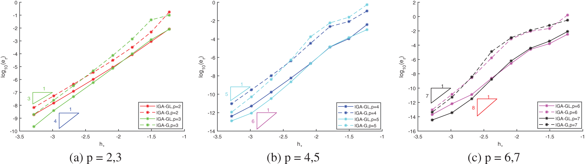
Figure 16: Convergence comparison between IGA-GL/IGA-G under different degrees of Example I
This study proposes a new perspective on solving IGA problems, which treats the left-hand side and right-hand side of the PDE as fitting the load function with the derivatives of the unknown NURBS-expressed solution. We present a detailed introduction to how to detect feature points on the load function of the PDE in 1D, 2D, and 3D cases. Then, we propose the IGA-CL method in which the knot vector of the NURBS numerical solution combines the characteristics of the load function with the representation of the physical domain. We validate that utilizing the feature points of the load function to construct the integrated knot vector helps improve the accuracy while generally maintaining the convergence rate. The theoretical result of the convergence behavior is beyond the scope of this study. Experimental results demonstrate that the accuracies of both our IGA-CL framework and IGA-GL framework are higher than those of the typical IGA-C and IGA-G methods, particularly in solving problems with analytical solutions with obvious characteristics.
Funding Statement: This work is supported by the National Natural Science Foundation of China under Grant Nos. 61872316, 62272406, 61932018, and the National Key R&D Plan of China under Grant No. 2020YFB1708900.
Conflicts of Interest: The authors declare that they have no conflicts of interest to report regarding the present study.
References
1. Hughes, T. J. R., Cottrell, J. A., Bazilevs, Y. (2005). Isogeometric analysis: CAD, finite elements, NURBS, exact geometry and mesh refinement. Computer Methods in Applied Mechanics & Engineering, 194(39), 4135–4195. [Google Scholar]
2. Zienkiewicz, O. C., Taylor, R. L. (2013). The finite element method: Its basis and fundamentals. Oxford: Butterworth-Heinemann. [Google Scholar]
3. Piegl, L., Tiller, W. (1997). The NURBS book. Berlin Heidelberg: Springer. [Google Scholar]
4. Auricchio, F., Beirão da Veiga, L., Hughes, T. J. R., Reali, A., Sangalli, G. (2010). Isogeometric collocation methods. Mathematical Models & Methods in Applied Sciences, 20(11), 2075–2107. https://doi.org/10.1142/S0218202510004878 [Google Scholar] [CrossRef]
5. Folland, G. B. (1995). Introduction to partial differential equations, vol. 102. Princeton, New Jersey: Princeton University Press. [Google Scholar]
6. Jupp, D. L. B. (1978). Approximation to data by splines with free knots. Siam Journal on Numerical Analysis, 15(2), 328–343. https://doi.org/10.1137/0715022 [Google Scholar] [CrossRef]
7. He, X., Shen, L., Shen, Z. (2002). A Data-adaptive knot selection scheme for fitting splines. IEEE Signal Processing Letters, 8(5), 137–139. [Google Scholar]
8. Lin, H., Hu, Q., Xiong, Y. (2013). Consistency and convergence properties of the isogeometric collocation method. Computer Methods in Applied Mechanics & Engineering, 267(8), 471–486. https://doi.org/10.1016/j.cma.2013.09.025 [Google Scholar] [CrossRef]
9. Anitescu, C., Yue, J., Zhang, Y. J., Rabczuk, T. (2015). An isogeometric collocation method using superconvergent points. Computer Methods in Applied Mechanics & Engineering, 284, 1073–1097. https://doi.org/10.1016/j.cma.2014.11.038 [Google Scholar] [CrossRef]
10. Quarteroni, A. (2017). Isogeometric analysis. In: Numerical models for differential problems. vol. 16. Cham: Springer. [Google Scholar]
11. Hughes, T. J. R., Reali, A., Sangalli, G. (2015). Efficient quadrature for NURBS-based isogeometric analysis. Computer Methods in Applied Mechanics & Engineering, 199(5), 301–313. [Google Scholar]
12. Barton, M., Calo, V. (2016). Gauss-Galerkin quadrature rules for quadratic and cubic spline spaces and their application to isogeometric analysis. Computer-Aided Design, 82, 57–67. https://doi.org/10.1016/j.cad.2016.07.003 [Google Scholar] [CrossRef]
13. Hiemstra, R. R., Calabrò, F., Schillinger, D., Hughes, T. J. R. (2017). Optimal and reduced quadrature rules for tensor product and hierarchically refined splines in isogeometric analysis. Computer Methods in Applied Mechanics & Engineering, 316, 966–1004. https://doi.org/10.1016/j.cma.2016.10.049 [Google Scholar] [CrossRef]
14. Wu, Z., Wang, S., Shao, W., Yu, L. (2020). Reusing the evaluations of basis functions in the integration for isogeometric analysis. Computer Modeling in Engineering & Sciences, 316(2), 459–485. https://doi.org/10.32604/cmes.2020.08697 [Google Scholar] [CrossRef]
15. Pan, M., Jüttler, B., Giust, A. (2020). Fast formation of isogeometric galerkin matrices via integration by interpolation and look-up. Computer Methods in Applied Mechanics & Engineering, 366, 113005. https://doi.org/10.1016/j.cma.2020.113005 [Google Scholar] [CrossRef]
16. Pan, M., Jüttler, B., Scholz, F. (2022). Efficient matrix computation for isogeometric discretizations with hierarchical B-splines in any dimension. Computer Methods in Applied Mechanics & Engineering, 388, 114210. https://doi.org/10.1016/j.cma.2021.114210 [Google Scholar] [CrossRef]
17. Cottrell, J. A., Reali, A., Bazilevs, Y., Hughes, T. J. R. (2006). Isogeometric analysis of structural vibrations. Computer Methods in Applied Mechanics & Engineering, 195(41), 5257–5296. https://doi.org/10.1016/j.cma.2005.09.027 [Google Scholar] [CrossRef]
18. Morganti, S., Auricchio, F., Benson, D. J., Gambarin, F. I., Hartmann, S. et al. (2015). Patient-specific isogeometric structural analysis of aortic valve closure. Computer Methods in Applied Mechanics & Engineering, 284, 508–520. https://doi.org/10.1016/j.cma.2014.10.010 [Google Scholar] [CrossRef]
19. Bouclier, R., Passieux, J. C. (2018). A Nitsche-based non-intrusive coupling strategy for global/local isogeometric structural analysis. Computer Methods in Applied Mechanics & Engineering, 340(1), 253–277. https://doi.org/10.1016/j.cma.2018.05.022 [Google Scholar] [CrossRef]
20. Bazilevs, Y., Calo, V. M., Zhang, Y., Hughes, T. J. R. (2006). Isogeometric fluid-structure interaction analysis with applications to arterial blood flow. Computational Mechanics, 38(4–5), 310–322. https://doi.org/10.1007/s00466-006-0084-3 [Google Scholar] [CrossRef]
21. Bazilevs, Y., Calo, V. M., Hughes, T. J. R., Zhang, Y. (2008). Isogeometric fluid-structure interaction: Theory, algorithms, and computations. Computational Mechanics, 43(1), 3–37. https://doi.org/10.1007/s00466-008-0315-x [Google Scholar] [CrossRef]
22. Seyfaddini, F., Nguyen-Xuan, H., Nguyen, V. H. (2021). A semi-analytical isogeometric analysis for wave dispersion in functionally graded plates immersed in fluids. Acta Mechanica, 232(3), 15–32. [Google Scholar]
23. Auricchio, F., Beirão da Veiga, L., Buffa, A., Lovadina, C., Reali, A. et al. (2007). A fully “locking-free” isogeometric approach for plane linear elasticity problems: A stream function formulation. Computer Methods in Applied Mechanics & Engineering, 197(1–4), 160–172. https://doi.org/10.1016/j.cma.2007.07.005 [Google Scholar] [CrossRef]
24. Elguedj, T., Bazilevs, Y., Calo, V. M., Hughes, T. J. R. (2010). B− and F− projection methods for nearly incompressible linear and non-linear elasticity and plasticity using higher-order NURBS elements. Computer Methods in Applied Mechanics & Engineering, 197(33), 2732–2762. [Google Scholar]
25. Benson, D. J., Bazilevs, Y., Hsu, M. C., Hughes, T. J. R. (2011). A large deformation, rotation-free, isogeometric shell. Computer Methods in Applied Mechanics & Engineering, 200(13), 1367–1378. https://doi.org/10.1016/j.cma.2010.12.003 [Google Scholar] [CrossRef]
26. Wolfgang, A., Frenzel, M. A., Cyron, C. (2008). Isogeometric structural shape optimization. Computer Methods in Applied Mechanics & Engineering, 197(33), 2976–2988. [Google Scholar]
27. Qian, X. (2010). Full analytical sensitivities in NURBS based isogeometric shape optimization. Computer Methods in Applied Mechanics & Engineering, 199(29), 2059–2071. https://doi.org/10.1016/j.cma.2010.03.005 [Google Scholar] [CrossRef]
28. Qian, X., Sigmund, O. (2011). Isogeometric shape optimization of photonic crystals via Coons patches. Computer Methods in Applied Mechanics & Engineering, 200(25), 2237–2255. https://doi.org/10.1016/j.cma.2011.03.007 [Google Scholar] [CrossRef]
29. Nguyen, V. P., Anitescu, C., Bordas, S. P. A., Rabczuk, T. (2015). Isogeometric analysis: An overview and computer implementation aspects. Mathematics & Computers in Simulation, 117, 89–116. https://doi.org/10.1016/j.matcom.2015.05.008 [Google Scholar] [CrossRef]
30. Schillinger, D., Evans, J. A., Reali, A., Scott, M. A., Hughes, T. J. (2013). Isogeometric collocation: Cost comparison with Galerkin methods and extension to adaptive hierarchical NURBS discretizations. Computer Methods in Applied Mechanics & Engineering, 13(1), 170–232. [Google Scholar]
31. Auricchio, F., Beirão da Veiga, L., Hughes, T. J., Reali, A., Sangalli, G. (2012). Isogeometric collocation for elastostatics and explicit dynamics. Computer Methods in Applied Mechanics & Engineering, 249–252(1), 2–14. https://doi.org/10.1016/j.cma.2012.03.026 [Google Scholar] [CrossRef]
32. Demko, S. (1985). On the existence of interpolating projections onto spline spaces. Journal of Approximation Theory, 43(2), 151–156. https://doi.org/10.1016/0021-9045(85)90123-6 [Google Scholar] [CrossRef]
33. Gomez, H., Lorenzis, L. D. (2016). The variational collocation method. Computer Methods in Applied Mechanics & Engineering, 309, 152–181. https://doi.org/10.1016/j.cma.2016.06.003 [Google Scholar] [CrossRef]
34. Montardini, M., Sangalli, G., Tamellini, L. (2017). Optimal-order isogeometric collocation at Galerkin superconvergent points. Computer Methods in Applied Mechanics & Engineering, 316, 741–757. https://doi.org/10.1016/j.cma.2016.09.043 [Google Scholar] [CrossRef]
35. Wang, D., Qi, D., Li, X. (2021). Superconvergent isogeometric collocation method with Greville points. Computer Methods in Applied Mechanics & Engineering, 377, 113689. https://doi.org/10.1016/j.cma.2021.113689 [Google Scholar] [CrossRef]
36. Atroshchenko, E., Gang, X., Tomar, S., Bordas, S. P. A. (2018). Weakening the tight coupling between geometry and simulation in isogeometric analysis: From sub-and super-geometric analysis to Geometry Independent Field approximaTion (GIFT). International Journal for Numerical Methods in Engineering, 114(10), 1131–1159. https://doi.org/10.1002/nme.5778 [Google Scholar] [CrossRef]
37. Beirão da Veiga, L., Lovadina, C., Reali, A. (2012). Avoiding shear locking for the Timoshenko beam problem via isogeometric collocation methods. Computer Methods in Applied Mechanics & Engineering, 241–244, 38–51. https://doi.org/10.1016/j.cma.2012.05.020 [Google Scholar] [CrossRef]
38. Auricchio, F., Beirão da Veiga, L., Kiendl, J., Lovadina, C., Reali, A. (2013). Locking-free isogeometric collocation methods for spatial Timoshenko rods. Computer Methods in Applied Mechanics & Engineering, 263(15), 113–126. https://doi.org/10.1016/j.cma.2013.03.009 [Google Scholar] [CrossRef]
39. Casquero, H., Liu, L., Bona-Casas, C., Zhang, Y., Gomez, H. (2016). A hybrid variational-collocation immersed method for fluid-structure interaction using unstructured T-splines. International Journal for Numerical Methods in Engineering, 105(11), 855–880. https://doi.org/10.1002/nme.5004 [Google Scholar] [CrossRef]
40. Morganti, S., Callari, C., Auricchio, F., Reali, A. (2018). Mixed isogeometric collocation methods for the simulation of poromechanics problems in 1D. Meccanica, 53, 1441–1454. https://doi.org/10.1007/s11012-018-0820-8 [Google Scholar] [CrossRef]
41. Morganti, S., Fahrendorf, F., Lorenzis, L. D., Evans, J. A., Hughes, T. et al. (2021). Isogeometric collocation: A mixed displacement-pressure method for nearly incompressible elasticity. Computer Modeling in Engineering & Sciences, 129(26), 1125–1150. https://doi.org/10.32604/cmes.2021.016832 [Google Scholar] [CrossRef]
42. Maurin, F., Greco, F., Coox, L., Vandepitte, D., Desmet, W. (2018). Isogeometric collocation for kirchhoff-Love plates and shells. Computer Methods in Applied Mechanics & Engineering, 329, 396–420. https://doi.org/10.1016/j.cma.2017.10.007 [Google Scholar] [CrossRef]
43. Pagani, L., Scott, P. J. (2018). Curvature based sampling of curves and surfaces. Computer Aided Geometric Design, 59(1), 32–48. https://doi.org/10.1016/j.cagd.2017.11.004 [Google Scholar] [CrossRef]
44. Filip, D., Magedson, R., Markot, R. (1986). Surface algorithms using bounds on derivatives. Computer Aided Geometric Design, 3(4), 295–311. https://doi.org/10.1016/0167-8396(86)90005-1. [Google Scholar] [CrossRef]
45. Park, H. (2004). An error-bounded approximate method for representing planar curves in B-splines. Computer Aided Geometric Design, 21(5), 479–497. https://doi.org/10.1016/j.cagd.2004.03.003 [Google Scholar] [CrossRef]
46. Razdan, A. (1999). Knot placement for B-spline curve approximation. In: Technical report. Tempe, AZ: Arizona State University. [Google Scholar]
47. Hernández-Mederos, V., Estrada-Sarlabous, J. (2003). Sampling points on regular parametric curves with control of their distribution. Computer Aided Geometric Design, 20(6), 363–382. https://doi.org/10.1016/S0167-8396(03)00079-7 [Google Scholar] [CrossRef]
48. Lu, L., Zhao, S. (2019). High-quality point sampling for B-spline fitting of parametric curves with feature recognition. Journal of Computational & Applied Mathematics, 345(1), 286–294. https://doi.org/10.1016/j.cam.2018.04.008 [Google Scholar] [CrossRef]
49. Schoenberg, I. J., Whitney, A. (1953). On Pólya frequency function. III: The positivity of translation determinants with an application to the interpolation problem by spline curves. Transactions of the American Mathematical Society, 74(2), 246–259. [Google Scholar]
50. Hosseini, S. F., Hashemian, A., Reali, A. (2020). Studies on knot placement techniques for the geometry construction and the accurate simulation of isogeometric spatial curved beams. Computer Methods in Applied Mechanics & Engineering, 360, 112705. https://doi.org/10.1016/j.cma.2019.112705 [Google Scholar] [CrossRef]
Cite This Article
 Copyright © 2023 The Author(s). Published by Tech Science Press.
This work is licensed under a Creative Commons Attribution 4.0 International License , which permits unrestricted use, distribution, and reproduction in any medium, provided the original work is properly cited.
 Downloads
 Citation Tools