COVID-19 Detection Based on 6-Layered Explainable Customized Convolutional Neural Network

1  Introduction

The new coronavirus has spread relatively quickly since its emergence. People may be infected unknowingly and cause greater damage to their bodies. Timely diagnosis of COVID-19 is crucial for disease control and patient care [1]. Nowadays, in addition to the confirmed patients, fast disease diagnosis [2] and proper treatment should be carried out quickly in the face of many suspected patients [3]. Therefore, how to do a good job of virus detection and quarantine has become a problem of public concern [4].

Although COVID-19 is a respiratory virus, it can affect the entire body, including the nervous system, bringing with it symptoms such as loss of taste and smell, headaches and strokes. It spreads rapidly and is highly insidious. Although testing methods vary from country to country and the frequency of testing varies, one thing is certain: rapid testing must be performed on anyone who shows symptoms of the virus and on those they have recently come into contact with. Currently, several countries and governments use RT-PCR test results as a standard for determining whether a patient has a case of COVID-19 virus. Collecting nucleic acid samples from a large number of residents for a long time is a great physical and mental drain on doctors or nurses. Recent studies show insufficient sensitivities and high false-negative rates for early diagnosis of presumptive patients [5]. Meanwhile, it may take up to 8–24 h and require multiple tests [6] for definite results [7]. Therefore, when patients exhibit respiratory symptoms [8], CT becomes a choice to help diagnose suspected COVID-19 patients. CT can avoid the problem of sample contamination compared to virus assay [9]; however, CT scans require an experienced doctor to make a diagnosis and always take a long time. As a disease of relatively short duration, COVID-19 may have similar symptoms and lesion images to other types of pneumonia. After the comparison of the COVID-19 group and the influenza pneumonia group, the COVID-19 group was more likely to have rounded opacities and interlobular septal thickening, but less likely to have nodules [10].

In the early stages of novel coronavirus pneumonia, the lesions are usually located unilaterally or bilaterally in the lung peripheral, showing multiple small patchy shadows and interstitial changes. As the infection further worsens, the lesion expands gradually, specifically in the form of bilateral multilobar or bilobar externally distributed lesions, with increased lesion components, which may appear as multiple ground-glass opacity [11] and infiltrative shadows. In severe cases, solid lung lesions may appear, and pleural effusions are rare.

In the face of the demand for testing a large number of samples every day, the manual detection method in the past is less efficient. However, with the development of computer technology, the convolutional neural network technology in machine learning can greatly improve the efficiency of sample detection. Efficient virus screening can reduce the human, material, financial and time input of hospitals and also win valuable treatment time for patients. This also places greater demands on the AI model, requiring the model to be explainable, allowing medical professionals to trust the machine applying the model and to take maximum advantage of artificial intelligence. In this paper, we use grad-cam plotting to obtain a heat map, which allows us to understand the basis of the model when classifying images and improves the clinical relevance of the model.

Many researchers are experimenting with the use of medical imaging to aid diagnosis. Wang et al. [12] proposed an optimized model to detect and classify COVID-19 cases from viral pneumonia [13] and X-ray images of the lungs of healthy people. Later, they proposed a PSSPNN to enable AI models to improve their performance compared to the nine state-of-the-art methods. In addition, a new AVNC model [14] is proposed, which takes the proposed VSBN as the backbone, integrating the attention mechanism and the improved multiplex data enhancement, and it shows that its sensitivity is all above 95% [15]. The paper [16] preprocessed chest X-ray images using an adaptive activation function [17] based U-Net, adding SA-TSA [18] to improve the performance of segmentation and detection, and finally completing lung segmentation. The comparison of the data listed by the authors in the paper indicates that the CNN model enhanced with SA-TSA achieves an accuracy of 0.970936 and a sensitivity of 0.957371, much higher than the other research methods in the table. This study [19] combined Pearson correlation [20] and K-nearest neighbour clustering [21] with convolutional neural networks and a decision tree [22] for accurate COVID-19 prediction. The experiments take advantage of the smaller error between the two variables to show that the provided method is superior to the traditional implementation. The MSE and RMSE values obtained from the experiments were 12.20 and 3.49 respectively. The paper [23] proposed a model that uses chest X-ray images containing multiple types of diseases as a dataset for multi-classification, combines GAN and LSTM for feature extraction, and achieves high accuracy. The model in the paper [24] also uses X-ray images as data, and uses both flat and hierarchical classification methods to obtain a new model, and compares the resulting model with other models in terms of generalisation ability.

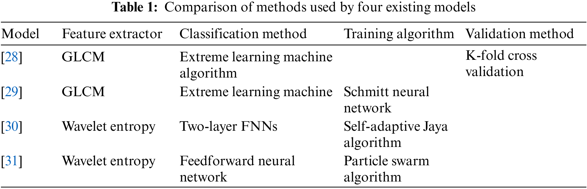
There are already some methods for classifying lung CT images for the COVID-19 diagnostic mission [25–27]. The paper [28] used GLCM to extract image features and then uses polarization to obtain classification results. The paper [29] pursued higher accuracy in the image preprocessing stage and used Schmidt neural network to complete the classification task after extracting texture features. The paper [30] verified the feasibility of the model based on WE and the adaptive algorithm for the classification task of COVID-19 chest CT images and achieved good results. The wavelet entropy was chosen as the feature extraction method in the paper [31], and a learning framework was constructed in combination with a feedforward neural network classifier. The adaptive particle swarm algorithm was used in the training process. Table 1 shows the comparison of methods used by four existing models.

Therefore, it is indispensable to use the extraction and analysis of COVID-19 image features to carry out artificial intelligence-assisted diagnosis. Once the trained model is obtained, we need to evaluate the performance of the model. The data in the dataset we are using is limited and using all the data in a single exercise to train the model can easily lead to overfitting, so we use K-fold cross validation. Ideally, we believe that K-fold cross-validation can be used to reduce the variance of the model by using a reasonable value of K, thus improving the generalisation ability of the model. This paper proposes 6L-CNN based on the convolutional neural network.

The rest of the paper is structured as follows. Section 2 shows the dataset. Section 3 describes the proposed 6-layer interpretable custom convolutional neural network model. Section 4 discusses the validation of our model using the K-fold validation method, comparing the results with other existing methods. In Section 5, we conclude the research of this paper.

2  Dataset

The dataset we used consisted of the COVID-19 patient group and the healthy group. All images have a resolution of 1024 × 1024 × 3. A total of 148 COVID-19 images and 148 healthy control (HC) images are obtained from reference [32]. Fig. 1 shows two figures in the dataset we used.

Figure 1: These two graphs are samples from the dataset

3  Methodology

Many fields have to face the problem of image classification. Manual extraction of features from images requires a strong understanding of the subject or the domain. Deep learning [33] is gradually becoming the primary tool for image classification tasks as performance improves over time [34]. Deep learning can automate the process of feature engineering. There are three important types of neural networks in deep learning: ANN, CNN, and RNN, which are the basis for many pre-trained models. ANN has a learning capacity [35,36]. ANN is mainly used to solve tabular text data. The inputs to ANN are only processed forward and cannot capture sequence information in the input data needed to process sequence data. Architecturally, RNNs have an additional cyclic connection on the hidden layer to ensure that sequential information is captured in the input data. RNNs are mainly used to solve problems related to time series data, text or audio data. CNNs are mainly used to solve problems related to image data and perform better on sequential inputs, so we chose CNNs as the basis of the model. Combining neural network(CNN) with medicine is a sure way to promote medical progress and human health [37].

CNN is a new type of network method that combines ANN and deep learning [38]. The CNN model adds a feature learning component to the original multilayer neural network so that it can be used to extract discriminative features from images for learning in fine classification recognition. Its derivative fields have been widely used in object segmentation, style conversion and other fields. Compared to traditional BP neural networks, CNN reduces the number of network parameters and enables weight sharing, thus making the network easy to optimize [39]. The CNN model is composed of five parts: the input layer, the convolutional layer, the pooling layer, the fully connected layer and the output layer. The CNN algorithm uses sparse connectivity and weight sharing to input images directly into the network, reducing the number of weights, facilitating network optimization, simplifying the model and reducing the risk of overfitting.

3.1 Convolutional Layer

In the convolutional neural network, several convolutional units form a convolutional layer. The parameters of each convolution unit are obtained by backpropagation. The function of the multiple convolutional layers [40,41] is to extract different input image features. By superimposing several convolutional layers, more complex features can be extracted iteratively from the edges and corners of the lower layers, making the image features more distinct. It not only highlights the features of the original signal but also reduces noise and facilitates the extraction of image features.

The image is stored in the computer as a pixel value. The extracted features are called convolutional kernels in CNN and can also be called filters. Overlay a filter on the original image, starting from the top left corner of the original image and moving sequentially to the right. The displacement of each movement of the filter is the stride size. The value of this filter is dotted with the pixel valueat the corresponding position after each move, and the resulting sum is the value of the target pixel in the output image. For every movement of the filter [42], a convolution is made. When the filter reaches the rightmost side, it moves to just below the initial position on the leftmost side of the row. The distance between the centre of the filter and the centre of the initial position of the previous row is equal to the stride size. The filter then continues to move to the right. The process is repeated continuously, ending when the filter reaches the bottom right corner of the image. This process is equivalent to the filter examining the entire image and finding features in the original image that are similar to those in the filter [43].

Some images may need to be padded during the convolution process for reasons such as different methods of convolution or inappropriate image and filter sizes. When convolution is performed, the edge features of the input image are computed less than the internal features, and the size of the output image becomes smaller in the convolution operation compared to the input image. Filling pixels along the edges of the input image is called padding. The padding illustration in Fig. 2 shows one layer of pixels around the input image, where padding = 1.

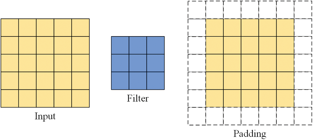
Figure 2: Input, filter, padding illustrations

Let the input image size be W×W, the filter size be F×F, the stride size be S, the number of layers of padded pixels around the input image be P, and the output size be N×N. The equation for the size of the convolved image is:

N=W−F+2PS+1(1)

There are three more commonly used convolution methods: full convolution, same convolution and valid convolution, shown in Fig. 3. These three methods have different restrictions on the range of movement of the convolution kernel. The full convolution starts when the filter and image just intersect. The same convolution is done when the centre of the filter coincides with the first pixel in the top left corner of the image. The same convolution is the most common type of convolution and is the one used in this paper. The same convolution allows the size of the feature map to be kept constant during forwarding propagation by adjusting the parameters, slowing down the rate of image shrinkage and preventing loss of boundary information. Valid convolution starts when the filter is all in the image.

Figure 3: Illustration of the three common convolution methods

3.2 Pooling Layer

The pooling layer after the convolution layer reduces the size of the input image, speeding up the computation and preventing overfitting. Among the several pooling methods available, the most popular are max pooling and average pooling [44]. Max pooling is the process of selecting a window of fixed size and placing the window over the original image, reserving the maximum value in the window. Slide the window to the right according to the stride size. After reaching the rightmost side of the image, return to the initial position, move down a distance equal to the stride size, continue sliding to the right and repeat the above operation until reaching the bottom right corner of the image. Finally, the max pooling result is obtained, as shown in Fig. 4.

Figure 4: Example of max pooling with a 2 × 2 filter and stride size = 2

Pooling does not change the number of channels. Max pooling saves the maximum value in each window, saving the result that best matches each window [45]. The average pooling follows a similar process to the maximum pooling process but keeps the average of all values in the window, as shown in Fig. 5.

Figure 5: Example of average pooling with a 2 × 2 filter and stride size = 2

3.3 ReLU Activation Function

After scanning the entire image with different filters, we apply an activation function to filter the output to introduce non-linearity. A neural network without a non-linear activation function would simply be a linear regression model. The complexity of regression models which use linear equations is limited and the ability to learn complex functional mappings from the data is inadequate. Adding a non-linear function increases the complexity of the model and allows arbitrarily complex functions to be mapped from the input to the output [46], learning and representing almost any neural network model. The activation function follows the output of the upper node and precedes the input of the lower node. Common activation functions are: Sigmoid function, Tanh function, ReLU function, ELU function. Fig. 6 shows the main parts of these functions.

Figure 6: Images of the four activation functions (x:y = 1:4)

The Sigmoid and tanh functions were once frequently used but have been dropped in recent years as they can lead to gradient explosion and gradient disappearance. ReLU is the most commonly used activation function, which converges much faster than sigmoid and tanh function and is faster to compute, but may result in a small number of parameters that can never be updated. The ELU function solved the problem of ReLU, but it is computationally intensive [47].

3.4 Structure of Key CNN

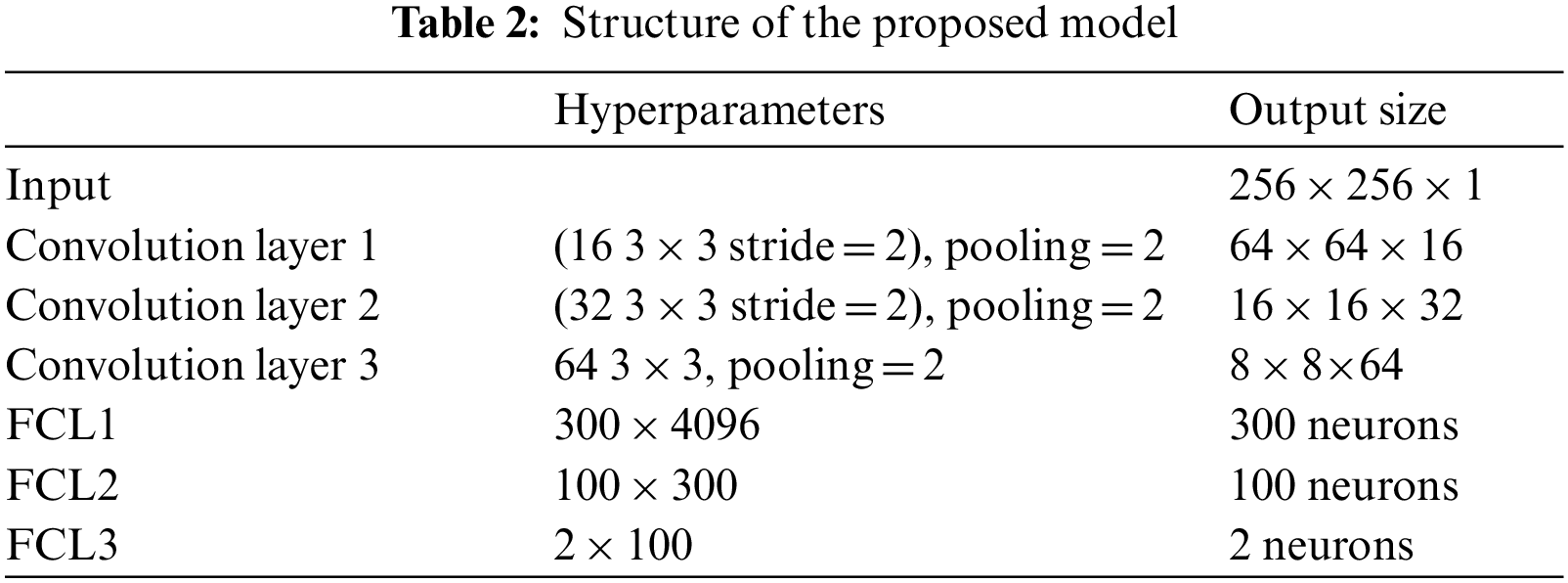
6L-CNN has six layers in total without the input layer. The input layer is the input to the whole neural network, a convolutional neural network processing images generally representing a matrix of pixels of an image [48]. Since the CT image we are using is a black and white image, the input layer has a depth of 1 and a size of 256 × 256. Con1 is the convolutional layer, using 16 3 × 3 filters and stride size = 2. After Con1 convolution, the image size is one-quarter of the original size, and the size of the output feature map is 128 × 128 × 16. Con1 is followed by a pooling layer with 2 × 2 filters and stride size = 2. The size of the resulting feature map is 64 × 64 × 16. Con2 is a convolution layer with 32 3 × 3 filters and stride size = 2. The image size after Con2 convolution is one-quarter of the original size. The size of the output feature map is 32 × 32 × 32. Con2 is followed by a pooling layer with 2 × 2 filters and stride size = 2. The size of the resulting feature map is 16 × 16 × 32. Con3 is a convolution layer with 64 3 × 3 filters and stride size = 1. The size of the output feature map is 16 × 16 × 64. Con3 is followed by a pooling layer with 2 × 2 filters and stride size = 2. The size of the resulting feature map is 8 × 8 × 64. The next three fully connected layers are 300 × 4096, 300 × 4096 and 2 × 100 in that order. The structure of this model is shown in Fig. 7 and Table 2.

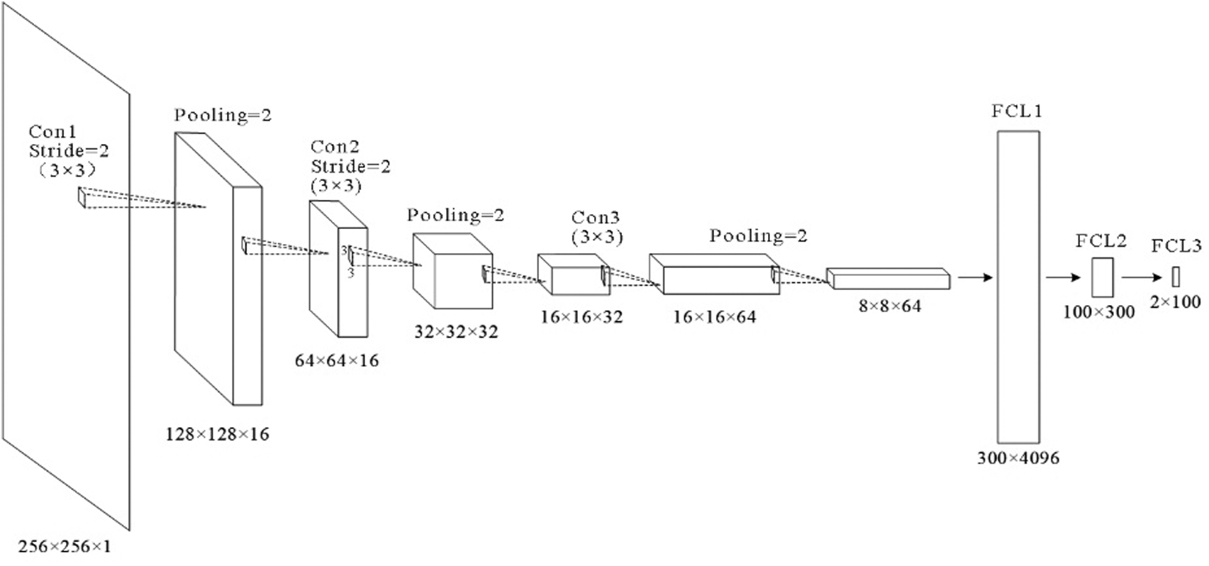
Figure 7: Structure of the proposed model

3.5 Explainability of Proposed Model

It is well known that deep learning as a representative of artificial intelligence technology has developed rapidly in recent years. Its achievements also have been widely used to improve people’s lives. However, due to the high technical requirements, it is difficult for managers and users to understand in practice. Researchers and developers also have a problem explaining it. When used as an aid system, the transparency and comprehensibility of the model are crucial. Only an intelligent system based on trust can take full advantage of the benefits of artificial intelligence. In comparison to the original cam, the grad-cam does not require any modification of the network structure and is more general and suitable for a wider range of scenarios. The purpose of using Grad-CAM is to visualize the basis on which the network classifies images. We use the regions of interest of the network to understand whether the model has a bias in learning and whether the learned category features are correct. We input an image from the dataset into the model. The last feature layer, F, is chosen for visualization as the position is further back in the feature layer the richer the feature information extracted. By back-propagating the final predicted value yA for category A, the gradient information F′ is back-propagated back to F. The importance level against each channel of F is obtained by averaging the gradient information F′ over each channel. Finally, we perform a simple weighted summation over the pass ReLU to obtain Grad-CAM.

The weight of the k th channel in the feature layer F of category A has the formula:

αkA=1Z∑i∑j∂yA∂Fijk(2)

yA represents the prediction of the network for category A, Fijk represents the feature layer F in channel k with coordinates at position ij, and Z is the result of the product of the height and width of the feature layer.

The formula for performing the weighted summation is:

Lgrad−camA=ReLU(∑kαkAFk)(3)

With the obtained heat map generated by the gram-cam, we can visualise the learning process of the model. Observing the model identifies the lesion area, thus determining the classification label of the image and knowing the way that the model is used to support accurate image classification. In clinical applications, it can provide valuable information to the physician for clinical identification, guide the clinical management of the patient. If the lesion area is too small, or the location is hidden, it may be overlooked by the physician when reading the CT image. Interpretable medical modeling of the lesion area can alert the physician to a more detailed examination. For the patient, a visualisation of his or her condition through the CT image can give him or her greater confidence in the doctor and in future treatment.

3.6 Cross Validation

As a statistical analysis method, cross validation can be used to select adjustment parameters, compare model performance differences, and select features. Cross validation is a powerful tool for guiding and validating research in artificial intelligence, machine learning, pattern recognition and classifiers [49].

The validation method we use is K-fold cross validation with K = 10, as shown in Fig. 8. K-fold cross validation is to divide the original data into K-folds, most of the time divided equally. Each fold is extracted once for the validation set, and the rest of the K-1 folds are used as the training set. After the subset has been extracted, it is put back and not repeated so that there are K different models. Each validation will result in a matching accuracy rate.

Figure 8: K-fold cross validation (K = 10)

The average accuracy Ei(i≤K) of these K models is used as the performance metric of this classifier. The method’s overall performance was then evaluated by calculating the mean e of the cross-validation indices.

e=110∑i=110Ei(4)

In order to observe how the model performs on each category, we use the confusion matrix, as shown in Fig. 9, to observe which of the categories are directly not easily distinguishable. For example, how many images were assigned to the wrong category, so that features etc. could be targeted to make the categories more distinguishable. Based on the confusion matrix, we can evaluate the performance of the model by calculating the values of Sensitivity (Sen), Spceficity (Spc), Priceision (Prc), Accuracy (Acc), F1, MCC and FMI.

Figure 9: The confusion matrix

The formulae used to calculate each data are as follows:

Sensitivity=TPTP+FN(5)

Specificity=TNFP+TN(6)

Accuracy=TP+TNTP+TN+FP+FN(7)

Precision=TPTP+FP(8)

MCC=TP×TN−FP×FN(TP+FP)×(TP+FN)×(TN+FP)×(TN+FN)(9)

F1=2TP2TP+FP+FN(10)

FMI=TP(TP+FP)×(TP+FN)(11)

4  Experiment Results and Discussions

4.1 The Results of the 6L-CNN

After validating the performance of 6L-CNN using 10-fold cross validation, Table 3 was obtained. The average sensitivity was 88.31 ± 1.83. The specificity was 89.53 ± 1.57. The precision was 89.43 ± 1.31. The accuracy was 88.92 ± 0.65. The F1 score was 88.85 ± 0.72. The MCC was 77.88 ± 1.30, and the FMI was 88.86 ± 0.71. The results of the observations show that the experiments performed well, with the performance metrics obtained being less far from the mean and with smaller standard deviations. The results fluctuate less for different subsets as validation sets. The accuracy fluctuations are minimal and the mean value is high, indicating that 6L-CNN classifies more accurately. Fig. 10 shows the linear table of the result 10-fold cross validation.

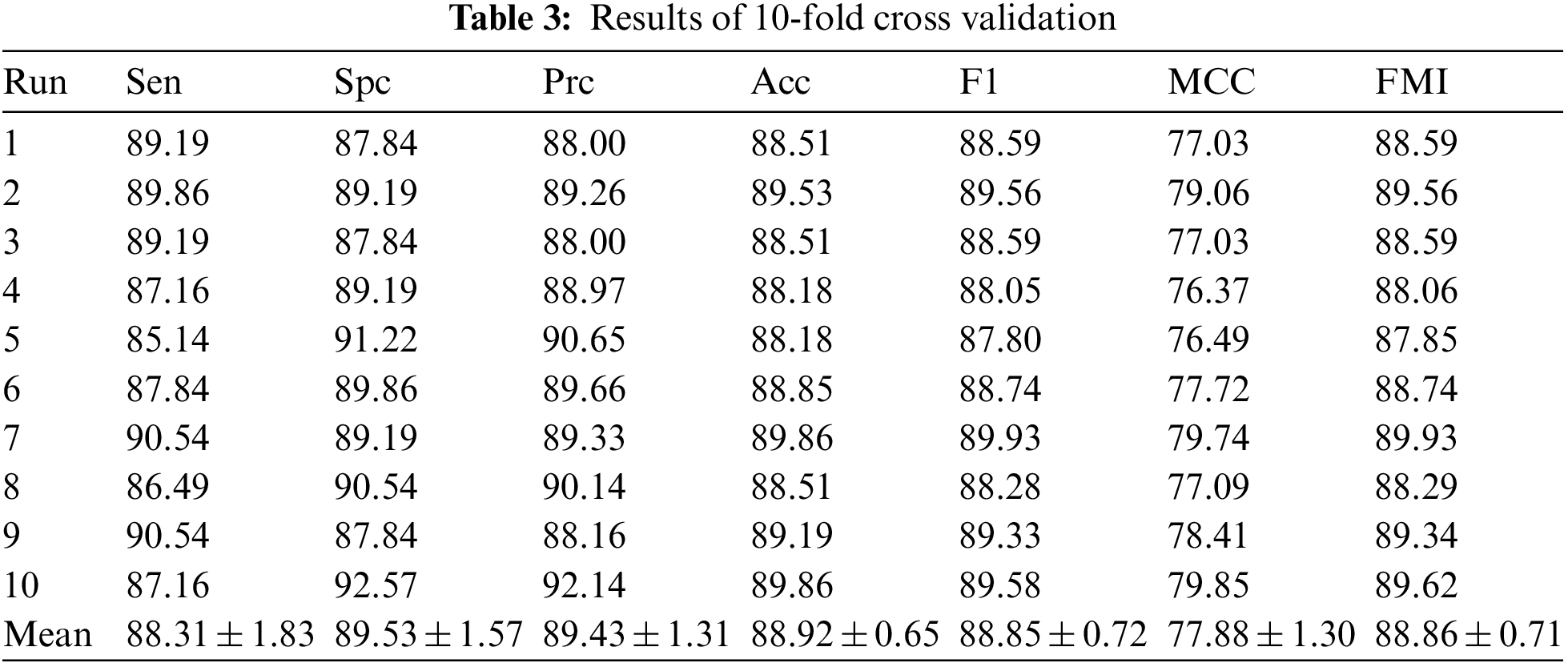
Figure 10: The linear table of the result 10-fold cross validation

4.2 Evaluation Criteria

Accuracy is one of the important criteria to evaluate the performance of a model. Fig. 11a shows the accuracy variation of 6L-CNN, and Fig. 11b is the keys of Fig. 11a. In fact, by the 4th epoch, we can see that the overall accuracy plateaus and remains at a high value.

Figure 11: The process of accuracy changes over 10 epochs of 6L-CNN

Confusion matric is often used in understanding the effect of classifiers to estimate the condition that whether the predicted category matches the actual category for each image. The confusion matrix provides a visual representation of the experimental results without losing the information. The confusion matrix for the 6L-CNN is shown in the top left corner of the figure. The first row of the matrix on the right is for the actual category of COVID-19, with 88.3% of the images being predicted correctly. The second row of the matrix on the right in the figure is for images with the actual category of health, and 89.5% of the images were predicted correctly. The left and right columns of each row add up to 100%. The matrix at the bottom of the figure focuses on the predicted results, with the percentages in each column summing to 100%. Of the images predicted to be COVID-19, 89.4% were in the actual category of COVID-19. Of the images with a predicted category of health, 88.5% match the actual category. The confusion matrices of 6L-CNN are shown in Fig. 12.

Figure 12: Confusion matrices of 6L-CNN

Common curves based on the confusion matrix are the PR curve and the ROC curve. In PR curves, P represents precision and R represents recall. The difference in the number of positive and negative samples in the dataset has a significant impact on the final PR curve graph. If the quantity variance is too large, the PR curve will change significantly and will be less stable. The ROC curve takes both positive and negative samples into consideration and is more stable. The horizontal coordinate of the ROC curve is the false positive rate (FPR) and the vertical coordinate is the true positive rate (TPR). We hope that the prediction accuracy of our proposed model will be as high as possible, which means that the TPR will increase. Meanwhile the lower the probability of false positives the better, which is a smaller FPR and closer to the origin. Fig. 13 shows the ROC curve of 6L-CNN.

Figure 13: ROC curve of 6L-CNN

4.3 Data Augmentation Results

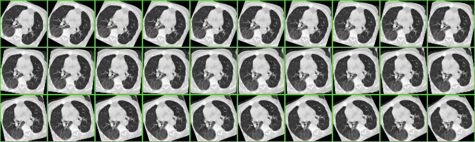
To increase the diversity of the images in the original sample dataset, we have added images (Appendix) based on the original images in the dataset that have been preprocessed in different methods. Processing methods include gamma correction, Gaussian noise, translation, rotation, and scaling. The gamma curve of the image in the original dataset is edited so that the proportion of dark and light parts of the image increases, thus improving the image contrast effect. Gaussian noise is the noise that appears in almost every pixel and has a random depth of noise. The images after Gaussian noise processing are simulated to be noisy due to random signal interference during acquisition and transmission. Translation, rotation and scaling are the three most basic image operations. These three methods do these operations on pixel values or coordinates of pixels to achieve a specific effect. Although these three methods are simple, they are very effective.

4.4 Structure Comparison

Multi-layer CNNs can learn to classify examples in some high-dimensional space, thus overcoming the limitation that single-layer neural networks can only be used to represent linearly separable functions. Determining the optimal number of layers for a CNN still requires ongoing experimental research. In order to get the best out of our model, we have set different numbers of layers for testing. We can observe the difference in the number of layers in Table 4 and in Fig. 14 drawn from the table. There is an increase in the effect of the model with each additional layer when the number of layers is increased from 4 to 6. When the number of layers is increased from 6 to 7, there is not only no increase but also a slight decrease in each indicator. After comparing the results, we found that the best results were obtained when the number of layers was 6.

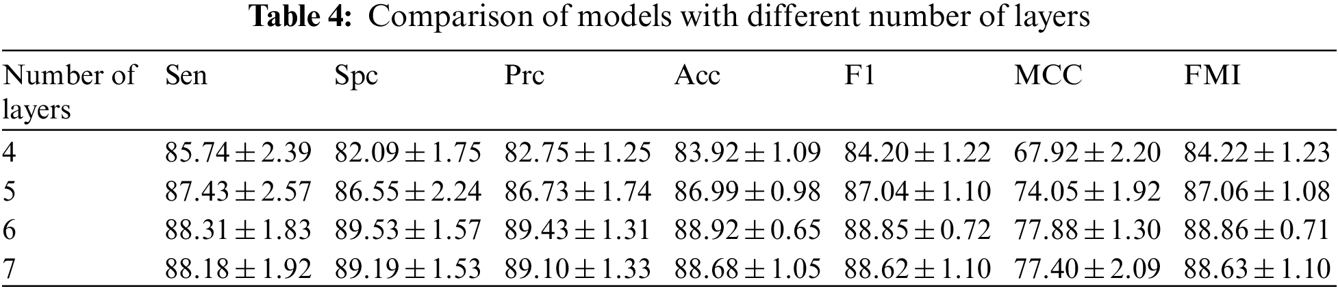
Figure 14: Model results for different number of layers

4.5 Comparison of State-of-the-Art Approaches

After 10 fold cross validation, we compared the obtained results for Sen, Spc, Prc, Acc, F1, MCC and FMI with those of the four existing methods, including GLCM-ELM, GLCM + SNN, WE-SAJ and WE-SaPSO, respectively. In terms of the average sensitivity of the ten validations, GLCM-ELM was 74.19%, GLCM + SNN was 74.80%, and WE-SAJ was 85.47%, WE-SaPSO was 85.14%, and 6L-CNN was 88.31%. 6L-CNN has the highest sensitivity and the least data fluctuation among the five methods, with stable performance.

In terms of accuracy, GLCM-ELM was 76%, GLCM + SNN was 76.22%, WE-SAJ was 86.35%, WE-SaPSO was 85.95%, and 6L-CNN was 88.92%. The data comparison shows that 6L-CNN not only has a more significant improvement in accuracy but is also more stable. The MCC scores were 52.08% for GLCM-ELM, 52.49% for GLCM + SNN, 72.75% for WE-SAJ, 71.95% for WE-SaPSO and 77.88% for 6L-CNN. Our method achieved the largest improvement of 25.8% compared to GLCM-ELM. We provide the results of comparison of four existing methods in Table 5 and a comprehensive comparison of all the performance in Fig. 15.

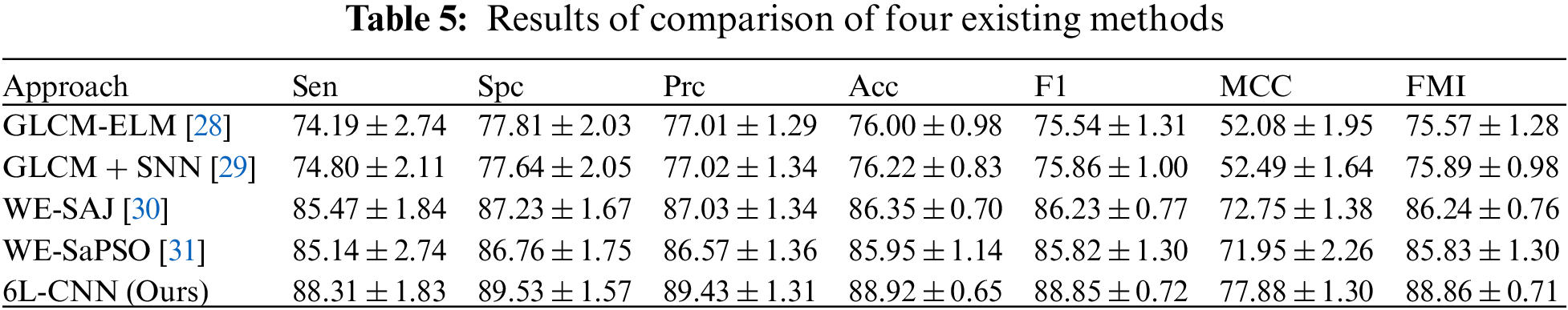
Figure 15: A comprehensive comparison of all the performance

Based on the above data, we have created a bar chart. Different metrics are represented by different colours. The graph shows that the corresponding metrics for each method have a similar trend of growth, and our proposed model for lung CT image classification has slightly better performance than the existing model in all aspects, especially in terms of improved accuracy and more stability.

4.6 Hyper-Parameter Tuning

In the process of adjusting hyperparameters, the best choice is to tune the most influential hyperparameter, the learning rate. As an important hyperparameter, setting it to the optimal value will help the model to achieve the best possible learning. If the learning rate is too small, the network will accumulate information too slowly, take too long to run and fall into a local minimum. A large learning rate is likely to result in a global minimum not being reached and a high loss. We wanted to balance the learning rate, learning effect, loss, and runtime. 6L-CNN was tried separately for training using different learning rates for each metric, the Table 6 was obtained and a line graph was drawn based on the table. From the Fig. 16, we find that the metrics with learning rates of 10−2 and 10−4 are slightly lower than those with learning rates of 10−3. The trend in each indicator as the learning rate increases is approximately the same. The learning rate of 10−3 is likely to be a turning point. Therefore, we finally chose to set the learning rate to 10−3 in the hyperparameter fine-tuning.

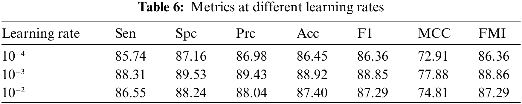
Figure 16: Trends in metrics for different learning rates for 6L-CNN settings

4.7 Explainability

To make our model explainable, we have drawn the following heat map by Grad-CAM. Observing the original CT image of the lung of the patient COVID-19, we can see a distinctive GGOs in the lower part of the left lung clearly. As described in Section 1, the GGOs is one of the main features of the CT image of the lungs of COVID-19 patients. In the heat map presented by Fig. 17c obtained by Grad-CAM, the red area is located in the lower part of the left lung, in the same position as the GGOs. This indicates that the network with learning believes that the image in the red region allows the 6L-CNN to make the final classification decision and is an important basis for the network to draw conclusions. This image also indicates a more accurate basis for the classification of our proposed model.

Figure 17: (a) Original CT image; (b) GGOs images are shown in red; (c) Grad-CAM image

5  Conclusions

In this paper, we used 6L-CNN to classify lung CT images of suspected cases to screen out patients with COVID-19. The method used to validate the model’s performance was the K fold cross-validation, and data were obtained for the model in terms of these metrics: specificity, accuracy, F1-score, MCC and FMI. In order to understand the progress of 6L-CNN in image classification, a comparison was made with four of the more current methods for advanced image classification, namely GLCM + SNN, WE-CSO, GLCM-ELM and WE-Jaya. The average sensitivity, specificity, precision, accuracy, F1-score, MCC and FMI of 6L-CNN were (88.31 ± 1.83%), (89.53 ± 1.57%), (89.43 ± 1.31%), (88.92 ± 0.65%), (88.85 ± 0.72%), (77.88 ± 1.30%) and (88.86 ± 0.71%). The results show that 6L-CNN is an improvement in all aspects compared to the four existing methods mentioned above and is more stable, which can better assist physicians in rapidly diagnosing patients with COVID-19 infection, isolating or treating them as early as possible and reducing the possibility of virus transmission.

In the future, we hope to incorporate attention mechanisms that will focus more attention on information that is more critical to the task. The limited attentional resources are used to quickly filter out the high-value information from the large amount of information. In terms of the structure of the neural network, the model we propose in this paper uses convolutional kernels of the same size, and in future research, we will try to use multiple convolutional kernels of different sizes to obtain features of different scales, and then combine these features. For the dataset direction, a combined analysis of X-ray images can be combined and the model is considered to be designed to have multiple inputs and to accept multiple types of medical images.

Funding Statement: This work was supported partly by the Open Project of State Key Laboratory of Millimeter Wave under Grant K202218, and partly by Innovation and Entrepreneurship Training Program of College Students under Grants 202210700006Y and 202210700005Z.

Conflicts of Interest: The authors declare that they have no conflicts of interest to report regarding the present study.

Appendix: Data Augmentation Results

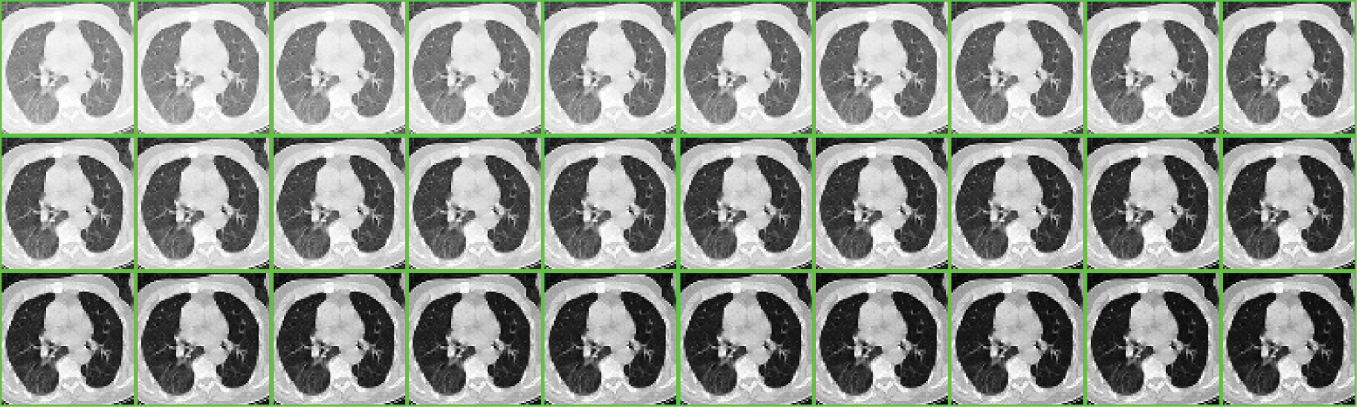
Partial images after Gamma Correction preprocessing

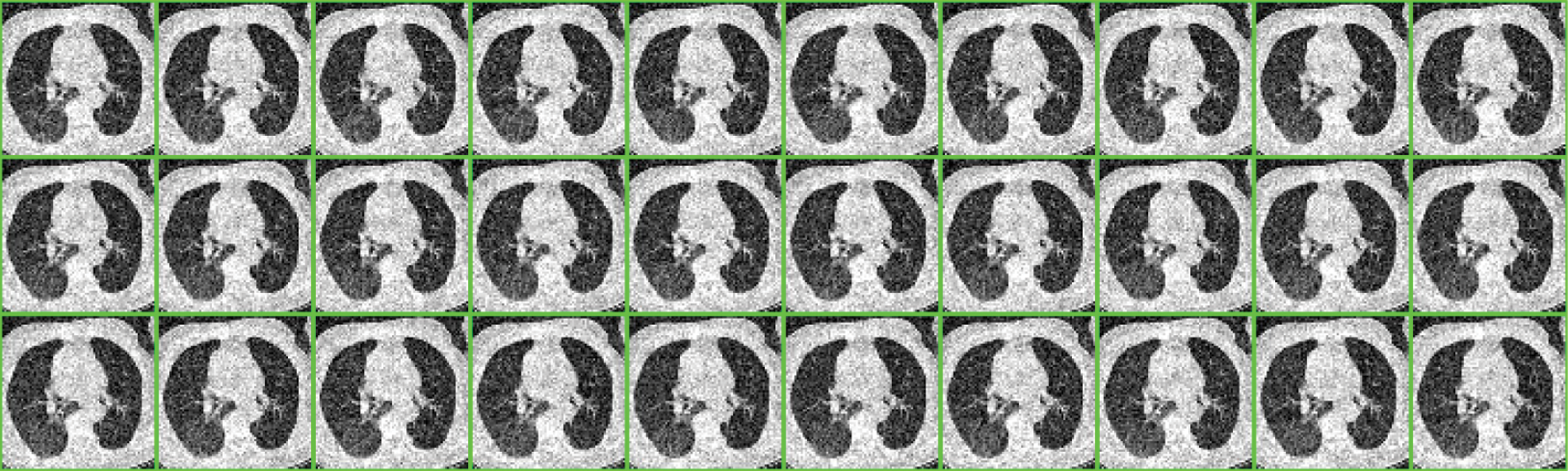
Partial images after Gaussian Noise preprocessing

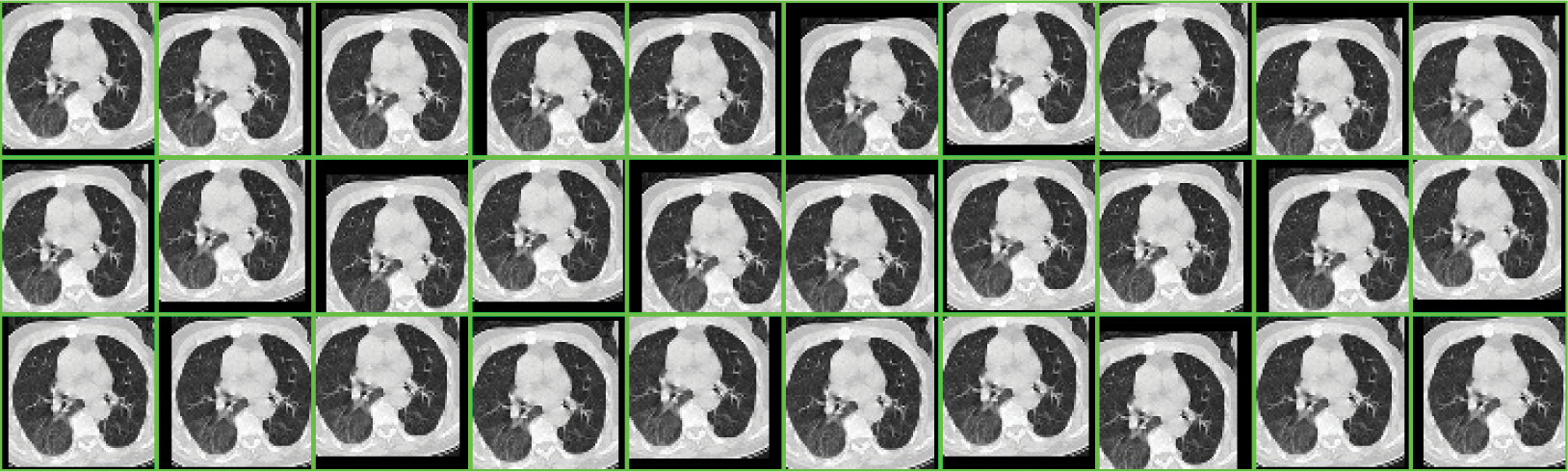
Partial images after Translation preprocessing

Partial images after Rotation preprocessing

Partial images after Scaling preprocessing

References

1. Dato, G. M. A. (2021). From COVID-19 or because COVID-19? Journal of Cardiac Surgery, 36(9), 3317–3318. https://doi.org/10.1111/jocs.15774 [Google Scholar] [PubMed] [CrossRef]
2. Lee, H. R. (2022). Predictors of red blood cell transfusion in elderly COVID-19 patients in Korea. Annals of Laboratory Medicine, 42(6), 659–667. https://doi.org/10.3343/alm.2022.42.6.659 [Google Scholar] [PubMed] [CrossRef]
3. Vuorio, A., Brinck, J., Kovanen, P. T. (2022). Continuation of fibrate therapy in patients with metabolic syndrome and COVID-19: A beneficial regime worth pursuing. Annals of Medicine, 54(1), 1952–1955. https://doi.org/10.1080/07853890.2022.2095667 [Google Scholar] [PubMed] [CrossRef]
4. Sencio, V., Benech, N., Robil, C., Deruyter, L., Heumel, S. et al. (2022). Alteration of the gut microbiota’s composition and metabolic output correlates with COVID-19-like severity in obese NASH hamsters. Gut Microbes, 14(1), 2100200. https://doi.org/10.1080/19490976.2022.2100200 [Google Scholar] [PubMed] [CrossRef]
5. Fang, Y., Zhang, H., Xie, J., Lin, M., Ying, L. et al. (2020). Sensitivity of chest CT for COVID-19: Comparison to RT-PCR. Radiology, 296(2), 115–117. https://doi.org/10.1148/radiol.2020200432 [Google Scholar] [PubMed] [CrossRef]
6. Capitelli, L., Bocchino, M., Giacon, V., Candia, C., Tafuro, F. et al. (2022). Correlations between viral load and symptoms in patient with COVID-19 pneumonia. Chest, 161(6), 140A–140A. https://doi.org/10.1016/j.chest.2021.12.172 [Google Scholar] [CrossRef]
7. Abduelkarem, A. R., Samorinha, C., Sharif, S. I., Hamrouni, A. M., Hassanein, M. M. (2022). Distress symptoms during the COVID-19 lockdown: A study with the general population of the United Arab Emirates. Pharmacy Practice, 20(2), 1–10. https://doi.org/10.18549/PharmPract.2022.2.2659 [Google Scholar] [PubMed] [CrossRef]
8. Rasoulinejad, S. A. (2022). Investigation of the clinical laboratory indexes in COVID-19 patients with ocular symptoms in Iran: A single-center experience. Archives of Pediatric Infectious Diseases, 10(3), e117175. https://doi.org/10.5812/apid [Google Scholar] [CrossRef]
9. Guo, X. (2022). A survey on machine learning in COVID-19 diagnosis. Computer Modeling in Engineering & Sciences, 130(1), 23–71. https://doi.org/10.32604/cmes.2021.017679 [Google Scholar] [CrossRef]
10. Liu, M., Zeng, W., Wen, Y., Zheng, Y., Lv, F. et al. (2020). COVID-19 pneumonia: CT findings of 122 patients and differentiation from influenza pneumonia. European Radiology, 30(10), 5463–5469. https://doi.org/10.1007/s00330-020-06928-0 [Google Scholar] [PubMed] [CrossRef]
11. Saha, M., Amin, S. B., Sharma, A., Kumar, T. K. S., Kalia, R. K. (2022). AI-driven quantification of ground glass opacities in lungs of COVID-19 patients using 3D computed tomography imaging. PLoS One, 17(3), e0263916. https://doi.org/10.1371/journal.pone.0263916 [Google Scholar] [PubMed] [CrossRef]
12. Wang, S. H., Zhang, Y., Cheng, X., Zhang, X., Zhang, Y. D. (2021). PSSPNN: PatchShuffle stochastic pooling neural network for an explainable diagnosis of COVID-19 with multiple-way data augmentation. Computational and Mathematical Methods in Medicine, 2021, 6633755. https://doi.org/10.1155/2021/6633755 [Google Scholar] [PubMed] [CrossRef]
13. Kör, H., Erbay, H., Yurttakal, A. H. (2022). Diagnosing and differentiating viral pneumonia and COVID-19 using X-ray images. Multimedia Tools and Applications, 81(27), 39041–39057. https://doi.org/10.1007/s11042-022-13071-z [Google Scholar] [PubMed] [CrossRef]
14. Burton, M. J., Ramke, J., Marques, A. P., Bourne, R. R. A., Congdon, N. et al. (2021). The lancet global health commission on global Eye health: Vision beyond 2020. The Lancet Global Health, 9(4), e489–e551. https://doi.org/10.1016/S2214-109X(20)30488-5 [Google Scholar] [PubMed] [CrossRef]
15. Wang, S. H., Nayak, D. R., Guttery, D. S., Zhang, X., Zhang, Y. D. (2021). COVID-19 classification by CCSHNet with deep fusion using transfer learning and discriminant correlation analysis. Information Fusion, 68, 131–148. https://doi.org/10.1016/j.inffus.2020.11.005 [Google Scholar] [PubMed] [CrossRef]
16. Das, A. (2022). Adaptive UNet-based lung segmentation and ensemble learning with CNN-based deep features for automated COVID-19 diagnosis. Multimedia Tools and Applications, 81(4), 5407–5441. https://doi.org/10.1007/s11042-021-11787-y [Google Scholar] [PubMed] [CrossRef]
17. Bodyanskiy, Y., Kostiuk, S. (2022). Adaptive hybrid activation function for deep neural networks. System Research and Information Technologies, 2022(1), 87–96. https://doi.org/10.20535/SRIT.2308-8893.2022.1.07 [Google Scholar] [CrossRef]
18. Kaur, S., Awasthi, L. K., Sangal, A., Dhiman, G. (2020). Tunicate swarm algorithm: A new bio-inspired based metaheuristic paradigm for global optimization. Engineering Applications of Artificial Intelligence, 90, 103541. https://doi.org/10.1016/j.engappai.2020.103541 [Google Scholar] [CrossRef]
19. Shinde, V., Bogiri, N. (2022). COVID-19 prediction through CNN and LSTM deep learning models. EasyChair [Google Scholar]
20. Muhaidat, J., Albatayneh, A., Abdallah, R., Papamichael, I., Chatziparaskeva, G. (2022). Predicting COVID-19 future trends for different european countries using Pearson correlation. Euro-Mediterranean Journal for Environmental Integration, 2022, 1–14. https://doi.org/10.1007/s41207-022-00307-5 [Google Scholar] [PubMed] [CrossRef]
21. Cunningham, P., Delany, S. J. (2021). K-nearest neighbour classifiers-A tutorial. ACM Computing Surveys, 54(6), 1–25 [Google Scholar]
22. Charbuty, B., Abdulazeez, A. (2021). Classification based on decision tree algorithm for machine learning. Journal of Applied Science and Technology Trends, 2(1), 20–28. https://doi.org/10.38094/jastt20165 [Google Scholar] [CrossRef]
23. Sheykhivand, S., Mousavi, Z., Mojtahedi, S., Yousefi Rezaii, T., Farzamnia, A. et al. (2021). Developing an efficient deep neural network for automatic detection of COVID-19 using chest X-ray images. Alexandria Engineering Journal, 60(3), 2885–2903. https://doi.org/10.1016/j.aej.2021.01.011 [Google Scholar] [CrossRef]
24. Luz, E., Silva, P., Silva, R., Silva, L., Guimarães, J. et al. (2021). Towards an effective and efficient deep learning model for COVID-19 patterns detection in X-ray images. Research on Biomedical Engineering, 38(1), 149–162. https://doi.org/10.1007/s42600-021-00151-6 [Google Scholar] [CrossRef]
25. Li, W., Deng, X., Shao, H., Wang, X. (2021). Deep learning applications for COVID-19 analysis: A state-of-the-art survey. Computer Modeling in Engineering & Sciences, 129(1), 65–98. https://doi.org/10.32604/cmes.2021.016981 [Google Scholar] [CrossRef]
26. Hou, S., Han, J. (2022). COVID-19 detection via a 6-layer deep convolutional neural network. Computer Modeling in Engineering & Sciences, 130(2), 855–869. https://doi.org/10.32604/cmes.2022.016621 [Google Scholar] [CrossRef]
27. Gu, X., Chen, S., Zhu, H., Brown, M. (2022). COVID-19 imaging detection in the context of artificial intelligence and the internet of things. Computer Modeling in Engineering & Sciences, 132(2), 507–530. https://doi.org/10.32604/cmes.2022.018948 [Google Scholar] [CrossRef]
28. Pi, P. (2021). Gray level co-occurrence matrix and extreme learning machine for COVID-19 diagnosis. International Journal of Cognitive Computing in Engineering, 2, 93–103. https://doi.org/10.1016/j.ijcce.2021.05.001 [Google Scholar] [CrossRef]
29. Pi, P. (2021). Gray level co-occurrence matrix and schmitt neural network for COVID-19 diagnosis. EAI Endorsed Transactions on e-Learning, 7(22), e3. https://doi.org/10.4108/eai.11-8-2021.170668 [Google Scholar] [CrossRef]
30. Wang, W., Zhang, X., Wang, S. H., Zhang, Y. D. (2022). COVID-19 diagnosis by WE-SAJ. Systems Science and Control Engineering, 10(1), 325–335. https://doi.org/10.1080/21642583.2022.2045645 [Google Scholar] [PubMed] [CrossRef]
31. Wang, W. (2022). COVID-19 detection by wavelet entropy and self-adaptive PSO. Lecture Notes in Computer Science, 13258, 125–135. https://doi.org/10.1007/978-3-031-06242-1 [Google Scholar] [CrossRef]
32. Zhang, Y. D. (2021). ANC: Attention network for COVID-19 explainable diagnosis based on convolutional block attention module. Computer Modeling in Engineering & Sciences, 127, 1037–1058. https://doi.org/10.32604/cmes.2021.015807 [Google Scholar] [CrossRef]
33. de Beurs, Z. L., Vanderburg, A., Shallue, C. J., Dumusque, X., Cameron, A. C. et al. (2022). Identifying exoplanets with deep learning. IV. Removing stellar activity signals from radial velocity measurements using neural networks. Astronomical Journal, 164(2), 49. https://doi.org/10.3847/1538-3881/ac738e [Google Scholar] [CrossRef]
34. Ragodos, R., Wang, T., Padilla, C., Hecht, J. T., Poletta, F. A. et al. (2022). Dental anomaly detection using intraoral photos via deep learning. Scientific Reports, 12(1), 1–8. https://doi.org/10.1038/s41598-022-15788-1 [Google Scholar] [PubMed] [CrossRef]
35. Mirak, S. H. M., Sharifian, S., Saraei, F. E. K., Asasian-Kolur, N., Haddadi, B. et al. (2022). Titanium-pillared clay: Preparation optimization, characterization, and artificial neural network modeling. Materials, 15(13), 4502. https://doi.org/10.3390/ma15134502 [Google Scholar] [PubMed] [CrossRef]
36. McCormick, M. (2022). An artificial neural network for simulation of an upflow anaerobic filter wastewater treatment process. Sustainability, 14(13), 7959. https://doi.org/10.3390/su14137959 [Google Scholar] [CrossRef]
37. Habibzadeh, M., Ameri, M., Haghighi, S. M. S., Ziari, H. (2022). Application of artificial neural network approaches for predicting accident severity on rural roads (Case study: Tehran-qom and Tehran-saveh rural roads). Mathematical Problems in Engineering, 2022, 5214703. https://doi.org/10.1155/2022/5214703 [Google Scholar] [CrossRef]
38. Zhang, Y. D. (2021). Improving ductal carcinoma in situ classification by convolutional neural network with exponential linear unit and rank-based weighted pooling. Complex & Intelligent Systems, 7, 1295–1310. https://doi.org/10.1007/s40747-020-00218-4 [Google Scholar] [PubMed] [CrossRef]
39. Yan, R. A., Zhang, L. C. (2021). Intrusion detection based on focal loss and convolutional neural network. Computer and Modernization, 2021(1), 65–69 [Google Scholar]
40. Kim, H. J., Kim, K. D., Kim, D. H. (2022). Deep convolutional neural network-based skeletal classification of cephalometric image compared with automated-tracing software. Scientific Reports, 12(1), 1–9. https://doi.org/10.1038/s41598-022-15856-6 [Google Scholar] [PubMed] [CrossRef]
41. Jedrzejczyk, A., Firek, K., Rusek, J. (2022). Convolutional neural network and support vector machine for prediction of damage intensity to multi-storey prefabricated RC buildings. Energies, 15(13), 4736. https://doi.org/10.3390/en15134736 [Google Scholar] [CrossRef]
42. Toma, R. N., Piltan, F., Im, K., Shon, D., Yoon, T. H. et al. (2022). A bearing fault classification framework based on image encoding techniques and a convolutional neural network under different operating conditions. Sensors, 22(13), 4881. https://doi.org/10.3390/s22134881 [Google Scholar] [PubMed] [CrossRef]
43. Wang, S. H. (2021). SOSPCNN: Structurally optimized stochastic pooling convolutional neural network for tetralogy of fallot recognition. Wireless Communications and Mobile Computing, 2021, 5792975. https://doi.org/10.1155/2021/5792975 [Google Scholar] [PubMed] [CrossRef]
44. Zhang, K. X., Liu, Y., Gu, Y., Ruan, X. J., Wang, J. D. (2022). Multiple-timescale feature learning strategy for valve stiction detection based on convolutional neural network. IEEE/ASME Transactions on Mechatronics, 27(3), 1478–1488. https://doi.org/10.1109/TMECH.2021.3087503 [Google Scholar] [CrossRef]
45. Guo, S. J., Kang, J. U. (2022). Convolutional neural network-based common-path optical coherence tomography A-scan boundary-tracking training and validation using a parallel monte carlo synthetic dataset. Optics Express, 30(14), 25876–25890. https://doi.org/10.1364/OE.462980 [Google Scholar] [PubMed] [CrossRef]
46. Sinha, S., Mishra, S., Mishra, V., Ahmed, T. (2022). Sector influence aware stock trend prediction using 3D convolutional neural network. Journal of King Saud University-Computer and Information Sciences, 34(4), 1511–1522. https://doi.org/10.1016/j.jksuci.2022.02.008 [Google Scholar] [CrossRef]
47. Lempart, M., Nilsson, M. P., Scherman, J., Gustafsson, C. J., Nilsson, M. et al. (2022). Pelvic U-Net: Multi-label semantic segmentation of pelvic organs at risk for radiation therapy anal cancer patients using a deeply supervised shuffle attention convolutional neural network. Radiation Oncology, 17(1), 1–15. https://doi.org/10.1186/s13014-022-02088-1 [Google Scholar] [PubMed] [CrossRef]
48. Wang, T. Y., Endo, M., Ohno, Y., Okada, S., Makikawa, M. (2022). Convolutional neural network-based computer-aided diagnosis in hiesho (cold sensation). Computers in Biology and Medicine, 145, 105411. https://doi.org/10.1016/j.compbiomed.2022.105411 [Google Scholar] [PubMed] [CrossRef]
49. Behera, S., Bhoi, S. S., Mishra, A., Nayak, S. S., Panda, S. K. et al. (2022). Comparative study of convolutional neural network and long short-term memory network for solar irradiance forecasting. Journal of Engineering Science and Technology, 17(3), 1845–1856 [Google Scholar]