Interpolation Technique for the Underwater DEM Generated by an Unmanned Surface Vessel

1  Introduction

A digital elevation model (DEM) is a mathematical representation of the continuously varying surface elevation within a certain area [1]. It provides fundamental data for use in geographic information systems (GIS) [2–6]. Transport via inland waterways is an important part of the integrated transport system in China and it is regarded as a “green” transport mode. An underwater DEM effectively reflects spatial information on the channel bed, and is one of the significant requirements for the normal operation of waterways. The information from underwater DEMs is widely used in water and soil conservation [7], hydrological analysis [8], river dredging [9], and environmental remediation [10,11]. The traditional method used to generate an underwater DEM is to measure underwater topographic points with tools, such as sextants, theodolites, and sounding rods. These methods are highly labor intensive, inefficient, imprecise, and pose a threat to the safety of operators. In recent years, unmanned surface vessels (USV) have been widely used in underwater topographic surveying and mapping. These can not only improve the accuracy of survey data, but also achieve a full-coverage survey of the underwater topography [12,13].

In practical applications, however, the distribution of USV measurement points is random and not consistent with the cross-section points of the river channel. Therefore, it is often necessary to use interpolation methods to estimate the elevation of unknown topographical points to obtain effective DEM data. Arun [14] used several interpolation methods to generate a DEM of the MANIT campus and surrounding areas of Bhopal in India and found that, in most contexts, kriging performed better than other contemporary methods. Nistora et al. [15] compared inverse distance weighted (IDW) and ordinary kriging (OK) to predict the groundwater table distribution; they found the results were quite similar. Observational data for the lower Danube was obtained by Diaconua et al. [16] to determine the best GIS interpolation method, and the result showed that both IDW and simple kriging provided satisfactory results. It can be concluded that in different measuring fields, the accuracy of the interpolation method has a strong correlation with the topographic features [17]. There is a need, therefore, to investigate the best interpolation methods for accurate and comprehensive underwater DEM information obtained by a USV.

This work used five different interpolation methods to generate an underwater DEM of the Panjing River in Shanghai, China, based on the channel topography measured by a USV. The characteristics of these interpolation methods were assessed and their interpolation precision in different terrains was analyzed using cross-validation. Based on the analysis results, an integrated interpolation approach was proposed for the generation of an underwater DEM in complex terrain with different surface roughness.

2  Interpolation Methods

Interpolation methods are widely applied in the construction of three-dimensional complex terrain [18,19]. In this section, five commonly-used interpolation methods are described.

2.1 Inverse Distance Weighted (IDW)

The IDW is a purely geometric weighted method and its algorithm is relatively simple and easy to operate. In the IDW method, the elevation value of an interpolated point P(x, y) is calculated by a linear weighted average. The weight λi is determined according to the distance between a measured point and an interpolated point di, which can be calculated through the spatial coordinates (x, y, z) of those points. Therefore, the closer the measured point is to the interpolated point, the greater the influence on the elevation value of the interpolated point. The expression of the IDW method is:

{P(x,y)=∑i=1nziλiλi=di−μ∑j=1ndj−μ(1)

where n is the number of the number of the adjacent measured points in the interpolation area that are used to calculate the elevation value of the interpolated point. μ is the power parameter that is usually set to be between 1 and 3 in the literature [20–22].

2.2 Ordinary Kriging (OK)

The principle of the OK method is very similar to that of IDW. It also estimates the elevation of the interpolated point through the weighted sum of the adjacent measured points in the area. However, in contrast to IDW, the spatial variance distribution of the measuring points is considered in the OK method to obtain the variant function. The variant function should satisfy the principles of both unbiasedness and the least estimated value. Common variant functions include the Gaussian model, exponential model, and spherical model [23–26]. After selecting the appropriate variant function, the elevations of the adjacent measured points are weighted to obtain the elevation of the interpolated point.

2.3 Radial Basis Function (RBF)

The RBF method is composed of three layers of neurons including the input layer, hidden layer and output layer. Its structure is shown in Fig. 1. This method ensures that the interpolation surface passes through all points and keeps the curvature to a minimum [27]. It is a combination of a series of precise interpolation methods. The input layer and output layer are both linear, and the hidden layer is a radial basis kernel function. The kernel function is one of the important factors affecting the interpolation precision. Commonly used functions include Gaussian kernel, polyquadratic surface, spline surface, and natural cubic spline surface [28–30].

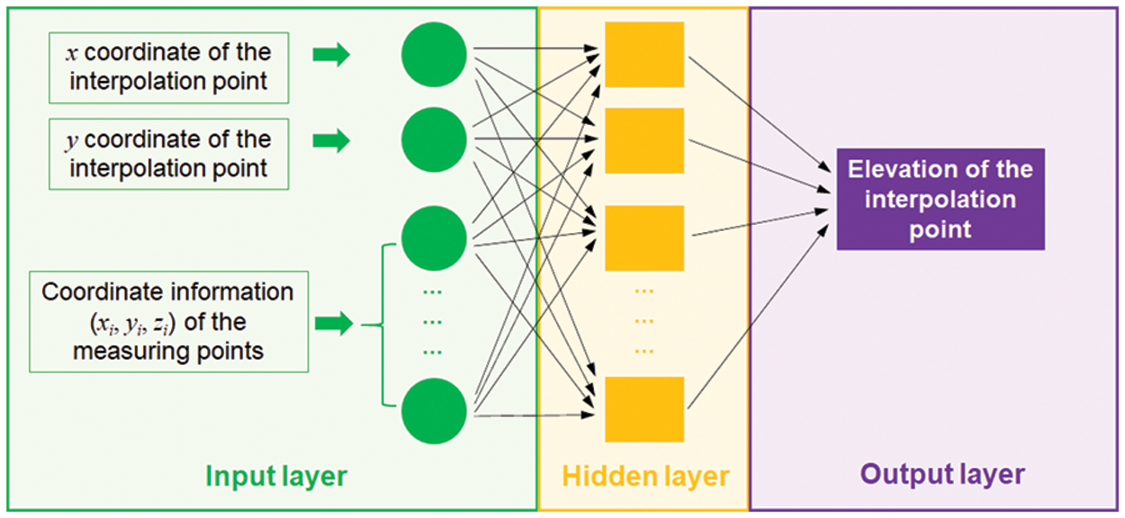
Figure 1: Algorithmic principle of the radial basis function (RBF) method

2.4 Moving Least Squares (MLS)

The MLS method is an interpolation algorithm that uses basis functions and fitting functions to segmentally fit the unknown surface. It can be expressed as:

P(x,y)=∑i=1nαi(x,y)qi(x,y)(2)

where P(x, y) represents the elevation of the interpolation point, and αi(x, y) is a function related to the spatial coordinates of the adjacent measured points. qi(x, y) is the basis function of MLS, which can generally be divided into a linear basis function and nonlinear basis function [31,32]. The basis function selected in this paper was the cubic spline function.

2.5 Triangulated Irregular Network (TIN)

The TIN method connects a series of discrete elevation points with connected and non-overlapping triangles, and forms a continuous triangular surface to describe three-dimensional terrain [33]. It can approximate the real terrain through different levels of resolution while maintaining the precision of the original data [31]. This means a TIN can provide an accurate representation of the original data and can effectively adapt to terrain irregularities because the elevation of each point is preserved, and the triangle defines a linear plane where new points can be inserted.

3  Accuracy Evaluation Indexes

For the purpose of model fitting, validation, and comparisons, the mean error (ME), root mean square error (RMSE), and regression coefficient (R2) have been used in a wide variety of disciplines, such as geosciences [34], atmospheric sciences [35], bio sciences [36]. In this work, these indexes were selected as indicators to evaluate the interpolation precision. These are expressed as:

ME=∑i=1n(Zi(x,y)−Pi(x,y))n,(3)

RMSE=∑i=1n(Zi(x,y)−Pi(x,y))2n,(4)

R2=1−∑i=1n(Zi(x,y)−Pi(x,y))2∑i=1n(Zi(x,y)−Pi_(x,y))2,(5)

where Zi(x, y) represents the predicted elevation value of the interpolated point, Pi(x, y) represents the measured elevation value, n represents the total number of samples in the inspection sample set, and P¯i (x, y) represents the average value of the measured elevation of all inspection sample points. The ME and RSME represent the absolute error between the measured and predicted value. The larger the ME and RMSE are, the greater the overall sample error. The R2 represents the dispersion degree of interpolation errors. If the R2 is close to 1, it means the interpolation error is concentrated.

4  Interpolation and Evaluation Analysis

4.1 Data Collection

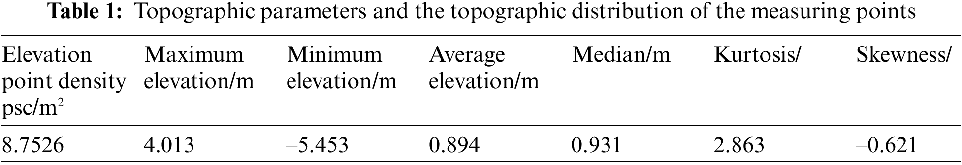
Panjing is a natural river located in the north of Shanghai, China (see Fig. 2). It stretches from Dijing in the south and flows through Luonan, Luodian and other areas. It is an important inland waterway in Shanghai, with a length of 19.0 km. In this work, an intelligent USV was used to measure the underwater topography of the Panjing River, as shown in Fig. 3. The size of this USV is 120 mm × 700 mm × 310 mm. The weight is about 26 kg, the maximum loading capacity is 15 kg, and the maximum cruising speed is 4.5 m/s. The USV was equipped with a dual-frequency GPS (horizontal accuracy of 10 mm ± 1 ppm, vertical accuracy of 20 mm ± 1 ppm) and a single-beam acoustic depth sounder (accuracy of 1 cm ± 0.1% × depth). The overall topographic parameters of the survey area and the topographic distribution of the measuring points are shown in Table 1.

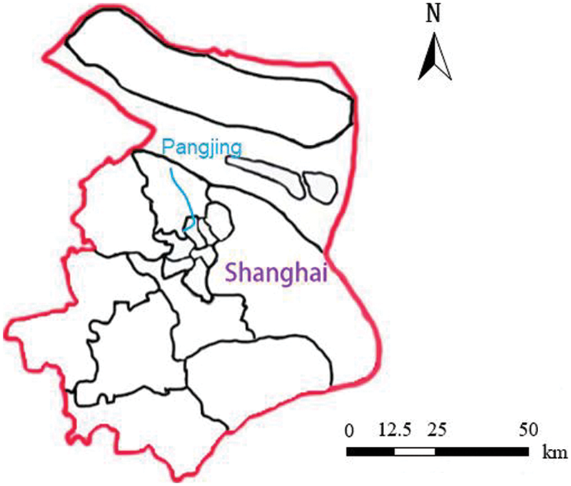
Figure 2: Location of the Panjing river

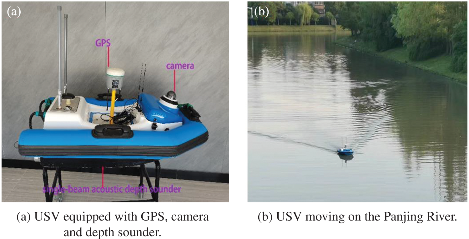
Figure 3: USV used to obtain the underwater elevation of the Panjing river

4.2 Data Processing

Global Positioning System (GPS) technology has been widely applied in a variety of engineering fields for positional fixes. However, due to atmospheric interference, satellite ephemeris errors and clock errors, errors are inevitable in the data collected by the GPS operating in the field. Therefore, the linear correction method proposed by Casaer et al. [37] was introduced in this study to improve the accuracy of GPS measurements.

To ensure the interpolation precision was comparable, the surveying area was divided into sub-sections every 50 m along the survey line. In total, 40 sample sections with uniformly distributed sampling points were selected. In this work, the Create Subsets function in the Geostatistics module in ArcGIS 10.5 (ESRI, Redlands, CA) was used to automatically extract 85% of the sample points as the interpolation sample data set, and the other 15% of the sample points as the verification data set. Cross-validation was used to evaluate the interpolation precision. According to the complex topographic features of inland river ways [38], surface roughness was selected as an index to describe the terrain of the sample sections. Surface roughness can reflect the undulation and erosion of terrain at a macroscopic scale [39–41]. It can be expressed as:

SR=1cos⁡(S×π180),(6)

where SR represents surface roughness, and S represents the average slope of the terrain in the section.

The five interpolation methods mentioned above were used to predict the underwater elevation of the test sample points in each sub-section. Then the predicted values were compared with the measured elevation values, and the three accuracy evaluation indicators were calculated for the different interpolation methods. The relationship between the interpolation accuracy and the surface roughness is shown in Fig. 4.

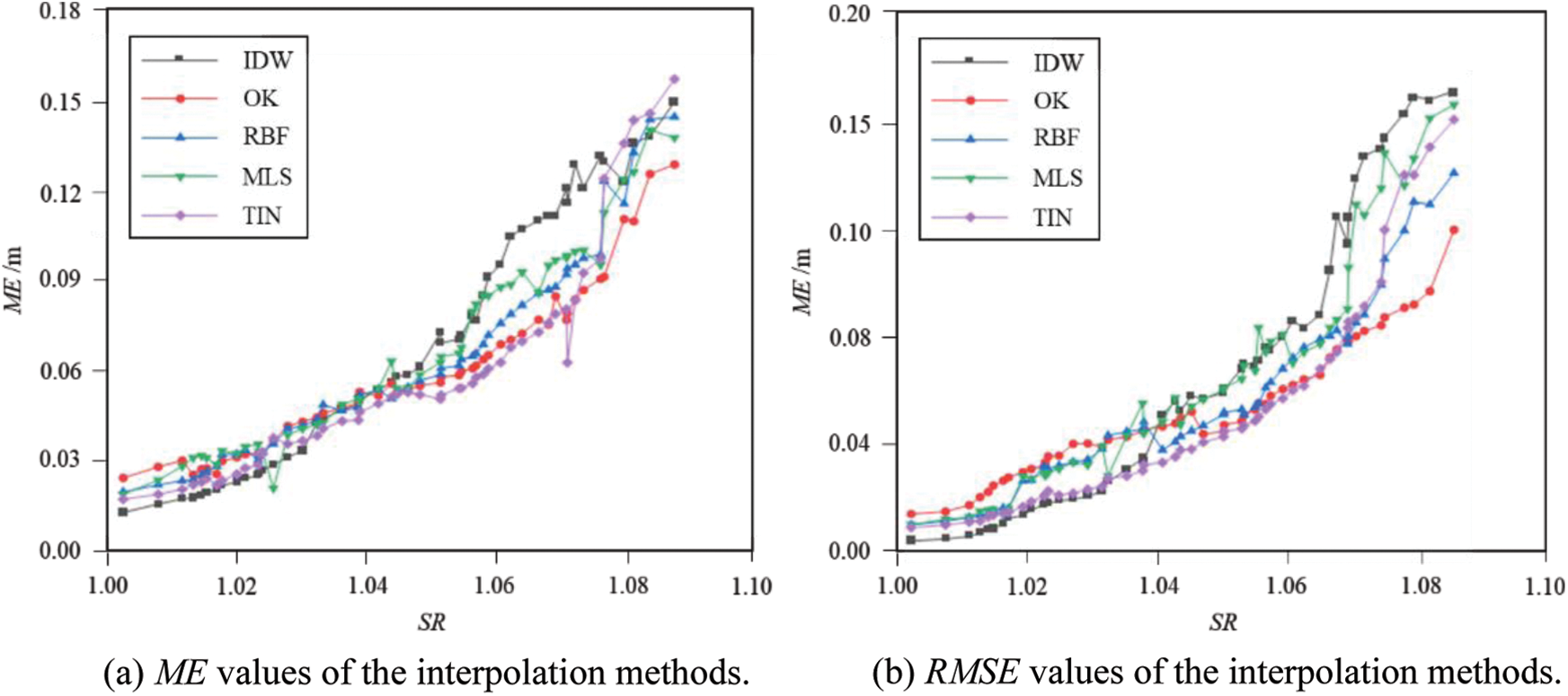
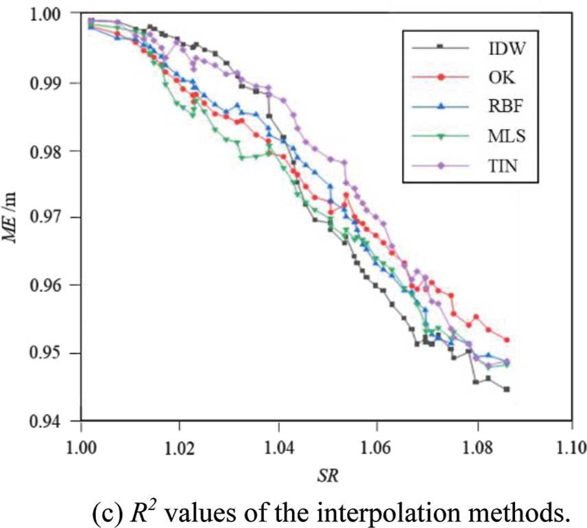
Figure 4: Comparison of accuracy indicators of the interpolation methods in relation to surface roughness

Fig. 4 shows a positive relationship between the interpolation error and the surface roughness of the river channel for each interpolation method. The results demonstrated that the higher the surface roughness was, the lower the accuracy of the interpolation model. When the surface roughness was less than 1.03, the interpolation precision of the different methods was relatively close. The highest interpolation precision was from IDW, followed by TIN. In this situation, the surface roughness had little effect on the interpolation accuracy. When the surface roughness was between 1.03 and 1.07, the difference in the precision between the interpolation methods gradually increased. The advantage of IDW was not obvious, and the performance of TIN interpolation was relatively stable. As the roughness increased, the RMSE and ME curves of the MLS method showed jump points; the accuracy change gradient was large, and the coincidence degree was relatively low. When the surface roughness was greater than 1.075, the accuracy of all the interpolation methods decreased even further. The interpolation accuracy was not stable except in the OK method. In some sections, the coincidence degree of the IDW method dropped below 0.95, which was lower than the confidence interval. In this interval, the OK method had the highest accuracy, followed by the RBF, while the IDW and TIN were the least accurate. Based on the above analysis, the optimal interpolation method for the survey area with different surface roughness is shown in Table 2.

4.3 Model Comparison

To further analyze the characteristics of each interpolation method for the underwater DEM, three typical survey areas with a surface roughness of 1.011, 1.048, and 1.083 were selected to compare the DEM interpolation results, as shown in Figs. 5–7.

Figure 5: Underwater DEM interpolation results in survey area No. 1 (surface roughness = 1.011)

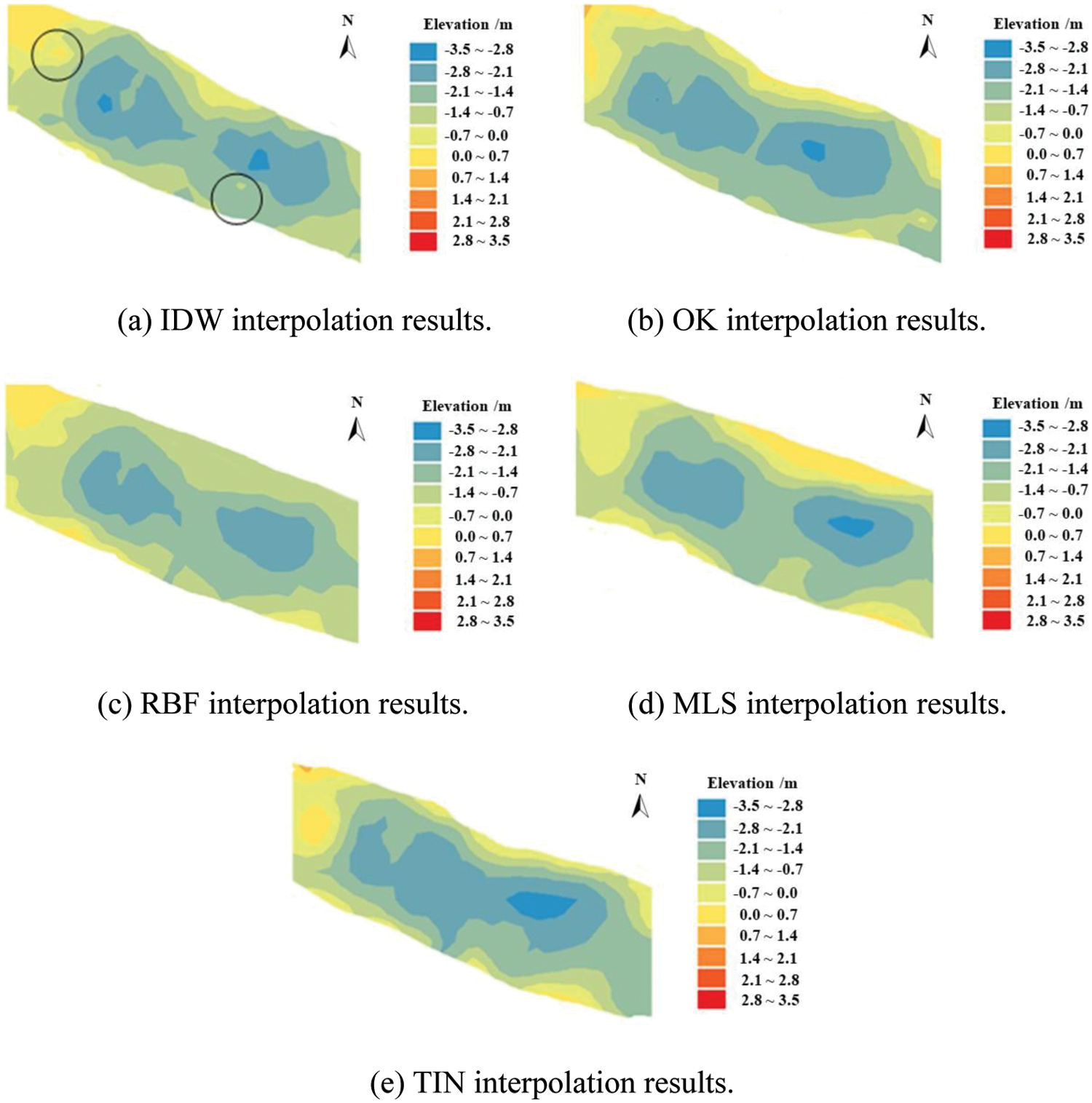
Figure 6: Underwater DEM interpolation results in survey area No. 2 (surface roughness = 1.048)

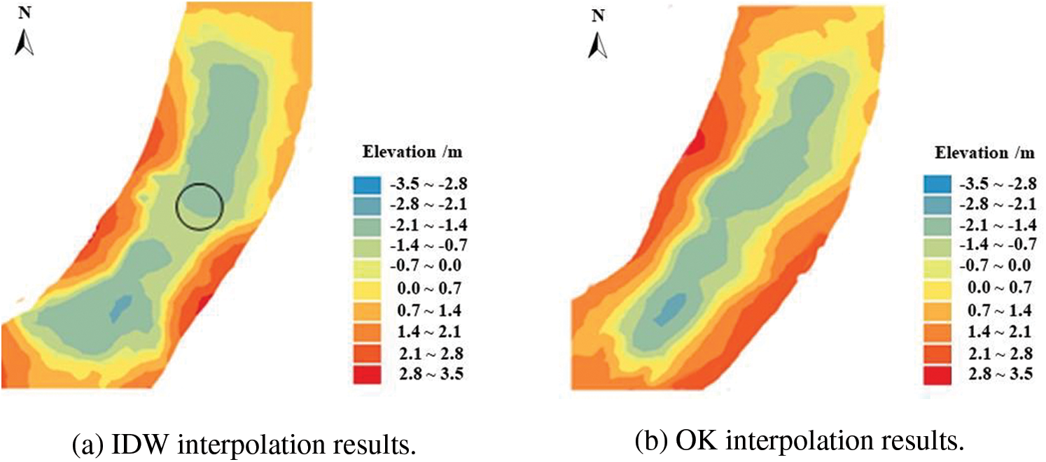
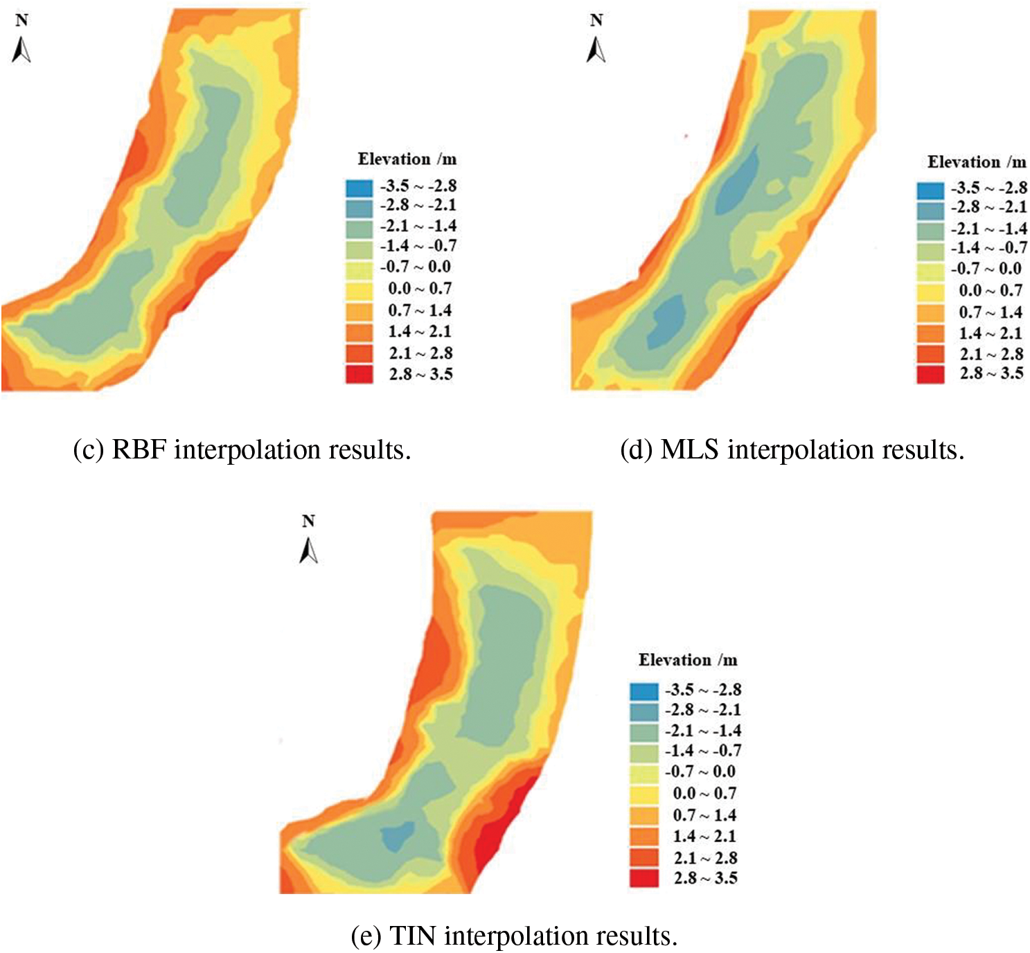
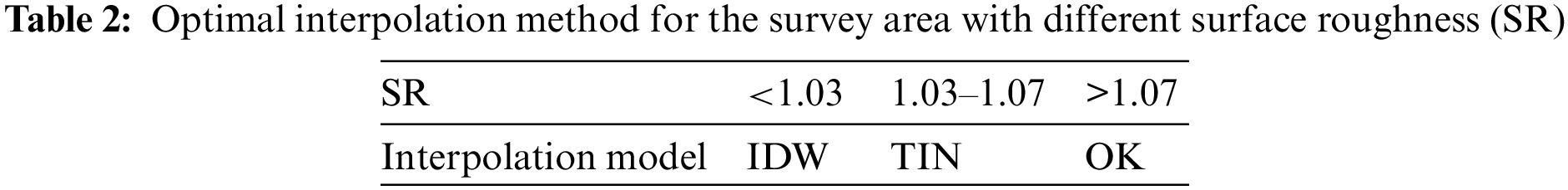
Figure 7: Underwater DEM interpolation results in survey area No. 3 (surface roughness = 1.083)

It can be seen from Figs. 3–5 that an increase in terrain surface roughness led to a corresponding reduction in the interpolation precision of each method. In the survey area No. 1 (SR = 1.011), the surface roughness was low and the topography was flat. The five interpolation methods had very close interpolation precision for the underwater DEM in this situation. With an increase in the surface roughness (SR = 1.048), the underwater DEM obtained by the five methods had significant differences, especially in the deeper channel area, but the generated river channel contour was still relatively similar. With a further increase in the surface roughness (SR = 1.083), the interpolation effect of each method was significantly affected by the terrain undulations, and there were sharp differences in the prediction of the channel topography. The contour distributions obtained by OK and MLS were relatively regular, but the topographic contours obtained by IDW, RBF, and TIN showed a crescent-shaped curve.

To investigate the characteristics of the different interpolation methods, the results were analyzed based on the interpolation principles of each method. The IDW method needed to ensure the uniformity of the sample point distribution during interpolation. However, it was difficult for the USV to maintain a constant speed during the survey. This may have caused insufficient sample points in one survey area, and excessive points in another area. This led to spherical protrusions (circled in Figs. 4 and 5), which are often called “bull’s eyes” in the literature. In addition, IDW only used the distance between the measured point and the estimated point as the weight indicator. Data smoothing was necessary during the weighting process, which may have resulted in lost detail. The disadvantages of TIN were similar with those of IDW. Because TIN used flat triangles to replace local topography in any terrain environment, the elevations of some points were smoothed in local hollows or silt deposition areas, which resulted in larger errors. Therefore, the interpolation accuracy of these two methods was higher in gentle areas, and lower in areas with complex terrain. In comparison, OK had stronger spatial adaptability than other interpolation methods because it could fully consider the spatial correlation of the overall topography of the survey area when selecting the variant function for interpolation. Moreover, its interpolation results were an optimal unbiased estimator, so that it could reduce the interpolation error caused by terrain variations and maintain strong interpolation robustness.

The MLS and RBF methods had no obvious advantages over the other methods. As a neural network algorithm, RBF had high interpolation precision and fast calculation speed, but it also had a strong dependence on the density of the sample points. However, the density of the measured points obtained by a USV may be relatively sparse, so there is little ability for training to allow the radial basis function to take maximum advantage of the interpolation algorithm. The MLS method first fitted a smooth surface and then interpolated the topographic points in the survey area. The selection of the fitting surface was controlled by a weight function, so that the shape of the surface could not be adaptively changed when the terrain varied. Therefore, the interpolation precision was significantly affected by terrain factors.

5  Integrated Interpolation Approach

Based on the above analysis, it was concluded that the different interpolation methods each had their own advantages and disadvantages, and their sensitivity to the variation in terrain was quite different. No single interpolation method was suitable for generating an underwater DEM in all terrain types. At present, the research on interpolation methods is mature and the theory is sound. It is probably not feasible to improve the algorithm structure of the traditional interpolation methods to control the errors in underwater DEMs. Therefore, this work proposed an integrated interpolation approach based on the interpolation characteristics of each method, which could automatically select the appropriate methods according to the different topographic surface roughness in the survey area and optimize the interpolation process. The integrated interpolation approach was divided into the following steps:

1)   The surveying area was divided into several sub-sections with similar areas and evenly distributed elevation points from the original survey line of the USV;

2)   Based on the topographic characteristics of the original survey points, the terrain surface roughness of each subsection was calculated, and used as an initial prediction of the underwater terrain pattern;

3)   The subsection in which the interpolation point was located was determined, and the appropriate interpolation method was selected according to the local surface roughness (Table 2) to obtain the underwater DEM.

In the traditional interpolation process, a single interpolation method is used for the DEM interpolation across an entire region. In the integrated approach proposed here, different interpolation methods are matched automatically to different terrain surface roughness in the interpolation process. Therefore, the respective advantages of different interpolation methods are optimized.

To verify the interpolation precision of the integrated approach, 15% of the measured elevation points were randomly selected from the samples as the testing sample set. Based on the analysis results in Table 2, the optimal interpolation method was automatically used to evaluate the elevation of those testing sample points. The three accuracy evaluation indexes (ME, RMSE, and R2) were calculated by comparing the interpolation result with the measured results using the Eqs. (3) to (5). The interpolation precision of the integrated approach was compared with the other five interpolation methods, and the results are shown in Fig. 8.

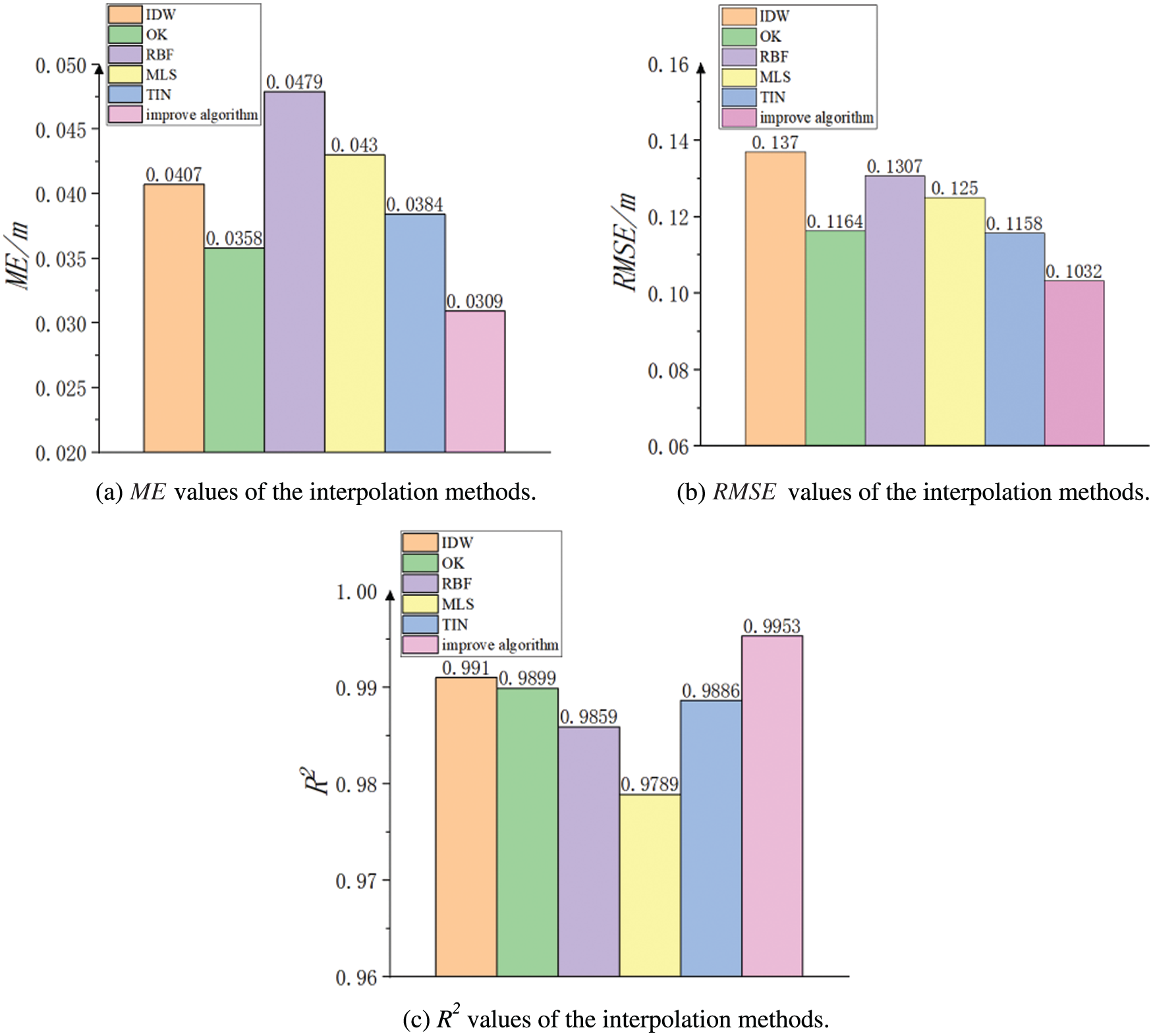
Figure 8: Comparison of the accuracy indicators of different interpolation methods

From the comparison in Fig. 6, it can be seen that when using one single interpolation method to estimate the overall testing sample points, the OK method was slightly better, followed by TIN. The overall sample error of IDW and RBF was larger, and the prediction coincidence of MLS was the lowest (0.9789).

From the perspective of the interpolation characteristics of the five methods, when using one single method to estimate the elevation of the sample points the interpolation precision largely depends on the variation of local terrain. Therefore, the applicability of different interpolation methods varies in different underwater terrain environments. The different sensitivities of the interpolation methods to the terrain variation weaken the natural attributes of the sample points if using a single method and are not be able to better represent the spatial distribution of nonlinear feature data. For example, when the IDW method performs elevation interpolation, it ensures that the estimated value of the interpolation point does not exceed the elevation range of the sample points and the generated DEM is smooth, but it causes some locally rugged terrain to be excessively smoothed, and the overall interpolation precision is reduced. In comparison, the presented integrated method can take full advantage of the different interpolation methods, reduce the overall interpolation error, and effectively restore the underwater terrain information. Fig. 6 shows that relative to a single method, the integrated method reduced the ME value by about 15% and the RMSE value by about 10% and increased the R2 value by about 0.005. Therefore, the integrated method has wider applicability.

6  Conclusions

On the basis of underwater terrain data of the Panjing River measured by a USV, this work introduced five different interpolation methods to generate an underwater DEM and analyzed the respective interpolation precision and interpolation effects under different spatial distributions. We found the following. 1) There was a positive spatial correlation between the interpolation errors and the terrain surface roughness. The interpolation precision decreased with the increase of the surface roughness. 2) The IDW method had a relatively high interpolation precision in flat areas (SR < 1.03). When the SR value ranged between 1.03 and 1.07, the TIN method had a better interpolation effect. The OK method maintained a higher interpolation precision when the terrain of the surveying area was complex, with a surface roughness value larger than 1.07.

On the basis of the analysis of the characteristics of the five interpolation methods, an integrated interpolation method was proposed to improve the interpolation precision. According to the topographic information reflected by the measured points in the survey area, the integrated approach automatically selected appropriate methods to predict the elevation of the interpolated points in the survey area according to different surface roughness. This approach is adaptive and can comprehensively use the advantages of the different interpolation methods and avoid the loss of information that can occur when describing the local terrain feature using a single interpolation method. Comparative analysis showed that the integrated approach improved the interpolation precision.

The presented results are limited to the Panjing River in Shanghai. The general applicability and reliability need to be further verified. In the next step, USV surveys will be carried out in different water systems to explore the specific scope of the application of the proposed integrated interpolation approach.

Funding Statement: The research work herein was supported by the National Natural Science Foundation of China (Grant No. 42102318) and the Program for Professor of Special Appointment (Eastern Scholar) at Shanghai Institutions of Higher Learning.

Availability of Data and Materials: The data used to support the findings of this study are included within the article.

Conflicts of Interest: The authors declare that they have no conflicts of interest to report regarding the present study.

References

1. Miky, Y., Kamel, A., Alshouny, A. (2022). A combined contour lines iteration algorithm and delaunay triangulation for terrain modeling enhancement. Geo-Spatial Information Science, 1–19. https://doi.org/10.1080/10095020.2022.2070553 [Google Scholar] [CrossRef]
2. Ghuffar, S. (2018). DEM generation from multi-satellite planet scope imagery. Remote Sensing, 10(9), 1462. https://doi.org/10.3390/rs10091462 [Google Scholar] [CrossRef]
3. Carlisle, B. H. (2005). Modelling the spatial distribution of DEM error. Transactions in GIS, 9(4), 521–540. https://doi.org/10.1111/j.1467-9671.2005.00233.x [Google Scholar] [CrossRef]
4. Hawker, L., Bates, P., Neal, J., Rougier, J. (2018). Perspectives on the digital elevation model (DEM) simulation for flood modeling in the absence of high-accuracy openaccess global DEM. Frontiers in Earth Science, 6, 233. https://doi.org/10.3389/feart.2018.00233 [Google Scholar] [CrossRef]
5. Lakshmi, S. E., Yarrakula, K. (2018). Review and critical analysis on digital elevation models. Geofizika, 35(2), 129–157. https://doi.org/10.15233/0352-3659 [Google Scholar] [CrossRef]
6. Natsagdorj, E., Renchin, T., Kappas, M., Tseveen, B., Dari, C. et al. (2017). An integrated methodology for soil moisture analysis using multispectral data in Mongolia. Geo-Spatial Information Science, 20(1), 46–55. https://doi.org/10.1080/10095020.2017.1307666 [Google Scholar] [CrossRef]
7. Smith, M. P., Zhu, A. X., Burt, J. E., Stiles, C. (2006). The effects of DEM resolution and neighborhood size on digital soil survey. Geoderma, 137(1–2), 58–69. https://doi.org/10.1016/j.geoderma.2006.07.002 [Google Scholar] [CrossRef]
8. Yusuf, S. M., Murtilaksono, K., Harjianto, M., Herlina, E. (2016). The utilization of satellite imagery data to predict hydrology characteristics in dodokan watershed. Procedia Environmental Sciences, 33, 36–43. https://doi.org/10.1016/j.proenv.2016.03.054 [Google Scholar] [CrossRef]
9. Ansari, S., Rennie, C. D., Seidou, O., Malenchak, J., Zare, S. G. (2017). Automated monitoring of river ice processes using shore-based imagery. Cold Regions Science and Technology, 142, 1–16. https://doi.org/10.1016/j.coldregions.2017.06.011 [Google Scholar] [CrossRef]
10. Wackerman, C., Hayden, A., Jonik, J. (2017). Deriving spatial and temporal context for point measurements of suspended-sediment concentration using remote-sensing imagery in the Mekong delta. Continental Shelf Research, 147, 231–245. https://doi.org/10.1016/j.csr.2017.08.007 [Google Scholar] [CrossRef]
11. Tanguy, M., Chokmani, K., Bernier, M., Poulin, J., Raymond, S. (2017). River flood mapping in urban areas combining radarsat-2 data and flood return period data. Remote Sensing of Environment, 198, 442–459. https://doi.org/10.1016/j.rse.2017.06.042 [Google Scholar] [CrossRef]
12. Hong, S., Kim, J. (2019). Three-dimensional visual mapping of underwater ship hull surface using view-based piecewise-planar measurements. IFAC PapersOnLine, 52(21), 384–389. https://doi.org/10.1016/j.ifacol.2019.12.337 [Google Scholar] [CrossRef]
13. Liu, Z. X., Yuan, C., Zhang, Y. M. (2015). Linear parameter varying adaptive control of an unmanned surface vehicle. IFAC PapersOnLine, 48(16), 140–145. https://doi.org/10.1016/j.ifacol.2015.10.271 [Google Scholar] [CrossRef]
14. Arun, P. V. (2013). A comparative analysis of different DEM interpolation methods. The Egyptian Journal of Remote Sensing and Space Sciences, 16, 133–139. https://doi.org/10.1016/j.ejrs.2013.09.001 [Google Scholar] [CrossRef]
15. Nistora, M. M., Rahardjoa, H., Satyanagaa, A., Haoa, K. Z., Qin, X. et al. (2020). Investigation of groundwater table distribution using borehole piezometer data interpolation: Case study of Singapore. Engineering Geology, 271, 105590. https://doi.org/10.1016/j.enggeo.2020.105590 [Google Scholar] [CrossRef]
16. Diaconua, D. C., Bretcanb, P., Peptenatua, D., Tanislavb, D., Mailatc, E. (2019). The importance of the number of points, transect location and interpolation techniques in the analysis of bathymetric measurements. Journal of Hydrology, 570, 774–785. https://doi.org/10.1016/j.jhydrol.2018.12.070 [Google Scholar] [CrossRef]
17. Oksanen, J., Sarjakoski, T. (2006). Uncovering the statistical and spatial characteristics of fine toposcale DEM error. International Journal of Geographical Information Science, 20(4), 345–369. https://doi.org/10.1080/13658810500433891 [Google Scholar] [CrossRef]
18. Guo, M., Zhou, Y., Zhao, J., Zhou, T., Yan, B. et al. (2021). Urban geospatial information acquisition mobile mapping system based on close-range photogrammetry and IGS site calibration. Geo-Spatial Information Science, 24(4), 558–579. https://doi.org/10.1080/10095020.2021.1924084 [Google Scholar] [CrossRef]
19. Crosby, H., Damoulas, T., Caton, A., Davis, P., Porto de Albuquerque, J. et al. (2018). Road distance and travel time for an improved house price kriging predictor. Geo-Spatial Information Science, 21(3), 185–194. https://doi.org/10.1080/10095020.2018.1503775 [Google Scholar] [CrossRef]
20. Chen, F. W., Liu, C. W. (2012). Estimation of the spatial rainfall distribution using inverse distance weighting (IDW) in the middle of Taiwan. Paddy and Water Environment, 10(3), 209–222. https://doi.org/10.1007/s10333-012-0319-1 [Google Scholar] [CrossRef]
21. Yang, X., Hodler, T. (2000). Visual and statistical comparisons of surface modeling techniques for point-based environmental data. Cartography and Geographic Information Science, 27(2), 165–175. https://doi.org/10.1559/152304000783547911 [Google Scholar] [CrossRef]
22. Macedonio, G., Pareschi, M. T. (1991). An algorithm for the triangulation of arbitrarily distributed points: Applications to volume estimates and terrain fitting. Computers & Geosciences, 17, 859–879. https://doi.org/10.1016/0098-3004(91)90086-S [Google Scholar] [CrossRef]
23. Keskin, H., Grunwald, S. (2018). Regression kriging as a workhorse in the digital soil mapper’s toolbox. Geoderma, 326, 22–41. https://doi.org/10.1016/j.geoderma.2018.04.004 [Google Scholar] [CrossRef]
24. Hengl, T., Heuvelink, G. B. M., Stein, A. A. (2004). Generic framework for spatial prediction of soil variables based on regression-kriging. Geoderma, 120, 75–93. https://doi.org/10.1016/j.geoderma.2003.08.018 [Google Scholar] [CrossRef]
25. Lark, R. M., Cullis, B. R., Welham, S. J. (2006). On spatial prediction of soil properties in the presence of a spatial trend: The empirical best linear unbiased predictor (E-BLUP) with REML. European Journal of Soil Science, 57, 787–799. https://doi.org/10.1111/j.1365-2389.2005.00768.x [Google Scholar] [CrossRef]
26. Lee, H., Choi, Y., Suh, J., Lee, S. H. (2016). Mapping copper and lead concentrations at abandoned mine areas using element analysis data from ICP-AES and portable XRF instruments: A comparative study. International Journal of Environmental Research and Public Health, 13, 384. https://doi.org/10.3390/ijerph13040384 [Google Scholar] [PubMed] [CrossRef]
27. Skala, V. (2017). RBF interpolation with CSRBF of large data sets procedia. Procedia Computer Science, 108, 2433–2437. https://doi.org/10.1016/j.procs.2017.05.081 [Google Scholar] [CrossRef]
28. Ghosh-Dastidar, S., Adeli, H., Dadmehr, N. (2008). Principal component analysis-enhanced cosine radial basis function neural network for robust epilepsy and seizure detection. IEEE Transactions on Biomedical Engineering, 55(2), 512–518. https://doi.org/10.1109/TBME.2007.905490 [Google Scholar] [PubMed] [CrossRef]
29. Wendland, H. (2006). Computational aspects of radial basis function approximation. Studies in Computational Mathematics, 12, 231–256. https://doi.org/10.1016/S1570-579X(06)80010-8 [Google Scholar] [CrossRef]
30. Majdisova, Z., Skala, V. (2017). Big geo data surface approximation using radial basis functions: A comparative study. Computers & Geosciences, 109, 51–58. https://doi.org/10.1016/j.cageo.2017.08.007 [Google Scholar] [CrossRef]
31. Ozkaya, S. I. (2002). CURVAZ—A program to calculate magnitude and direction of maximum structural curvature and fracture-flow index. Computers & Geosciences, 28, 399–407. https://doi.org/10.1016/S0098-3004(01)00050-4 [Google Scholar] [CrossRef]
32. de Baar, J., Dwight, R. P., Bijl, H. (2013). Speeding up kriging through fast estimation of the hyperparameters in the frequency-domain. Computers & Geosciences, 54, 99–106. https://doi.org/10.1016/j.cageo.2013.01.01 [Google Scholar] [CrossRef]
33. Ivanov, V. Y., Vivoni, E. R., Bras, R. L., Entekhabi, D. (2004). Catchment hydrologic response with a fully distributed triangulated irregular network model. Water Resources Research, 40(11), W11102. https://doi.org/10.1029/2004WR003218 [Google Scholar] [CrossRef]
34. Khosravi, K., Shahabi, H., Pham, B. T., Adamawoski, J., Shirzadi, A. et al. (2019). A comparative assessment of flood susceptibility modeling using multi-criteria decision-making analysis and machine learning methods. Journal of Hydrology, 573, 311–323. https://doi.org/10.1016/j.jhydrol.2019.03.073 [Google Scholar] [CrossRef]
35. Ji, F., Ekström, M., Evans, J. P., Teng, J. (2014). Evaluating rainfall patterns using physics scheme ensembles from a regional atmospheric model. Theoretical and Applied Climatology, 115 (1–2), 297–304. https://doi.org/10.1007/s00704-013-0904-2 [Google Scholar] [CrossRef]
36. Ameri, H., Yousefi, M., Yaseri, M., Nahvijou, A., Arab, M. et al. (2019). Mapping the cancer-specific QLQ-C30 onto the generic EQ-5D-5L and SF-6D in colorectal cancer patients. Expert Review of Pharmacoeconomics & Outcomes Research, 19 (1), 89–96. https://doi.org/10.1080/14737167.2018.1517046 [Google Scholar] [PubMed] [CrossRef]
37. Casaer, J., Hermy, M., Coppin, P. (1999). Appropriateness of the linear correction method for GPS positional fixes in wildlife studies. Wildlife Biology, 5(2), 125–128. https://doi.org/10.2981/wlb.1999.009 [Google Scholar] [CrossRef]
38. Wise, S. (2011). Cross-validation as a means of investigating DEM interpolation error. Computers & Geosciences, 37(8), 978–991. https://doi.org/10.1016/j.cageo.2010.12.002 [Google Scholar] [CrossRef]
39. Kidron, G. J., Tal, S. Y. (2012). The effect of biocrusts on evaporation from sand dunes in the Negev desert. Geoderma, 179(180), 104–112. https://doi.org/10.1016/j.geoderma.2012.02.021 [Google Scholar] [CrossRef]
40. Bullard, J. E., Ockelford, A., Strong, C. L., Aubault, H. (2018). Impact of multi-day rainfall events on surface roughness and physical crusting of very fine soils. Geoderma, 313, 181–192. https://doi.org/10.1016/j.geoderma.2017.10.038 [Google Scholar] [CrossRef]
41. Chamizo, S., Rodríguez-Caballero, E., Román, J. R., Cantón, Y. (2017). Effects of biocrust on soil erosion and organic carbon losses under natural rainfall. Catena, 148, 117–125.https://doi.org/10.1016/j.catena.2016.06.017 [Google Scholar] [CrossRef]
Cite This Article
Copyright © 2023 The Author(s). Published by Tech Science Press.
This work is licensed under a Creative Commons Attribution 4.0 International License , which permits unrestricted use, distribution, and reproduction in any medium, provided the original work is properly cited.
Downloads
Citation Tools