
 Submit a Paper
 Propose a Special lssue
 Open Access
ARTICLE

Chaotic Motion Analysis for a Coupled Magnetic-Flow-Mechanical Model of the Rectangular Conductive Thin Plate
1
School of Civil Engineering, Anhui Jianzhu University, Hefei, 230601, China
2
Key Laboratory of Intelligent Underground Detection Technology, Anhui Jianzhu University, Hefei, 230601, China
* Corresponding Author: Xiaofang Kang. Email:
(This article belongs to the Special Issue: Vibration Control and Utilization)
Computer Modeling in Engineering & Sciences 2023, 137(2), 1749-1771. https://doi.org/10.32604/cmes.2023.027745
Received 13 November 2022; Accepted 13 February 2023; Issue published 26 June 2023
 View Full Text
 Download PDF
Abstract
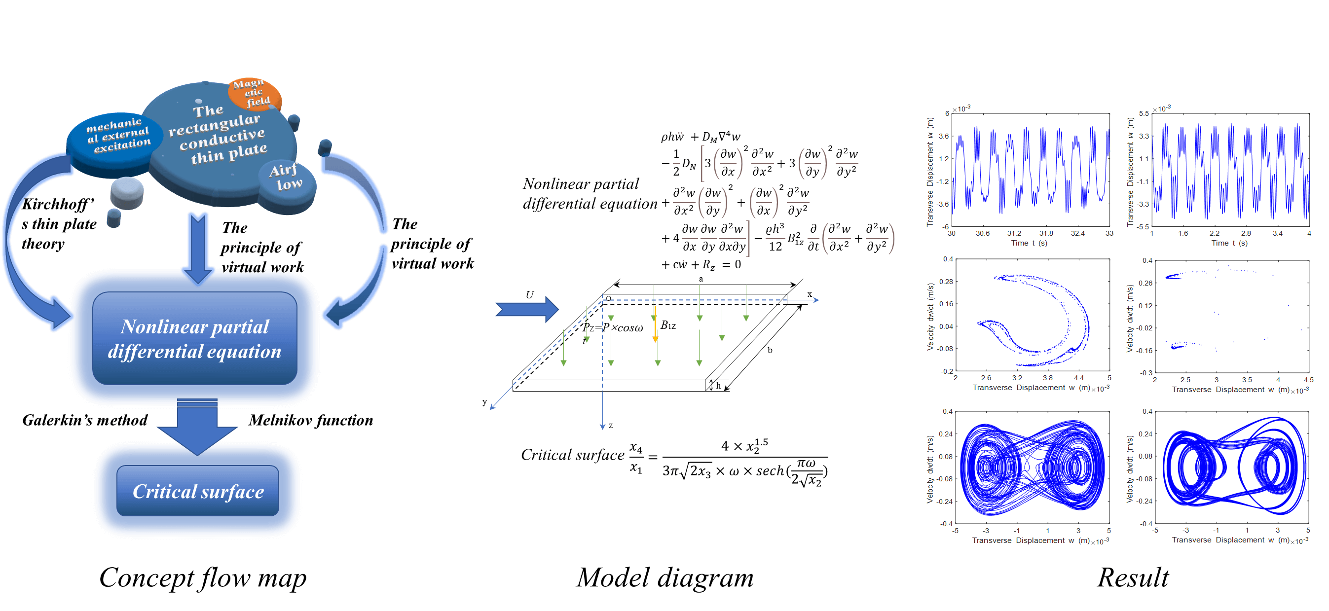
The chaotic motion behavior of the rectangular conductive thin plate that is simply supported on four sides by airflow and mechanical external excitation in a magnetic field is studied. According to Kirchhoff ’s thin plate theory, considering geometric nonlinearity and using the principle of virtual work, the nonlinear motion partial differential equation of the rectangular conductive thin plate is deduced. Using the separate variable method and Galerkin’s method, the system motion partial differential equation is converted into the general equation of the Duffing equation; the Hamilton system is introduced, and the Melnikov function is used to analyze the Hamilton system, and obtain the critical surface for the existence of chaos. The bifurcation diagram, phase portrait, time history response and Poincaré map of the vibration system are obtained by numerical simulation, and the correctness is demonstrated. The results show that when the ratio of external excitation amplitude to damping coefficient is higher than the critical surface, the system will enter chaotic state. The chaotic motion of the rectangular conductive thin plate is affected by different magnetic field distributions and airflow.Graphic Abstract
Keywords
With the advancement and development of modern high-tech, devices with magnetic, electrical, and other materials as structures are frequently used. Rectangular thin plates are widely used in road and bridge construction, machinery industry, ship engineering, aerospace, and other fields. When the system is disturbed by the outside world, it will not only produce periodic linear dynamic behavior, but also show chaotic motion behavior to a large extent, resulting in the failure of the system under repeated loads. At present, there are two very popular directions for the study of nonlinear dynamics of structures such as thin plates at home and abroad. One is the study of nonlinear aeroelastic problems, the other is the study of nonlinear electromagnetic elasticity aspects.
The study of geometric nonlinear aeroelasticity differs from general aeroelasticity [1] from the theoretical aspects as follows: One is the structural geometric nonlinear theory, which mainly addresses the static and dynamic analysis of the structure under large deformation [2–4]; The other is the study of surface aerodynamic theory [5], which mainly addresses the boundary condition dependent deformation state aerodynamic calculation method under large deformation conditions of the structure [6]; The third is the study of the structural/aerodynamic interface coupling method [7,8], which mainly investigates the multidimensional interpolation problem applicable to large deformation in space. The problem of subsonic aeroelasticity of plates focuses on the fluid-structure coupling between the structure and the airflow [9,10]. The variety of parameters, such as mass, damping and stiffness of the structure under the action of subsonic airflow affects the critical instability and nonlinear vibration characteristics of the structure [2,11]. The assumption of small deformation in its research is no longer applicable, the equilibrium state of the structure after force deformation presents obvious geometric differences relative to the undeformed structure, and the geometric nonlinear factors caused by the load-bearing and deformation state of the structure make the structural static and dynamic characteristics change, and change the static and dynamic aeroelastic coupling relationship, thus making the research and application of aeroelasticity face new challenges.
The theory of electromagnetic elasticity is devoted to the study of the coupling of electromagnetic fields with deformation fields. This theory is basically a coupling of the theory of linear elasticity [12] and the theory of linear electrodynamics in a free moving medium. If the studied elastomer is located in an initially strong magnetic field, mechanical and thermal loads would generate an electromagnetic field while causing a deformation field. The two fields will interact and influence each other and a coupling mechanism will occur. The action of the electromagnetic field on the deformation field is caused by the Lorentz force in the equations of motion [13–15]. The deformation field affects the strength of the magnetic field, the magnetoelastic wave [16] and the propagation velocity of the electromagnetic wave, and the item depends on the displacement velocity of the deformed object in the magnetic field [17]. Extensive research on the theory of magnetoelastic nonlinear problems in electromagnetic structures is important for the dynamic analysis of structural elements at high temperatures [18–20], high pressures and under the action of strong electromagnetic fields. For example, Liu et al. [21,22] performed numerical simulations using the pseudo-arclength continuation algorithm to analyze the effects of external temperature variations, magnetic potential, electrical potential, and excitation amplitude on the nonlinear vibration response of composite cylindrical shells. When the electromagnetic structure is in an applied electromagnetic field environment, on one hand, the electromagnetic structure is deformed by the electromagnetic force [23,24], and on the other hand, the deformation of the structure leads to a change in the electromagnetic field and thus to a change in the distribution of the electromagnetic force. For the current-carrying conductor [25], the electromagnetic force is the Lorentz force. For polarizable or magnetizable electromagnetic dielectric materials, the electromagnetic force is generated by the interaction of the polarization or magnetization [26] with the external electromagnetic field. A fundamental feature of this mutual coupling of the electromagnetic and mechanical fields is the nonlinearity. Even if the electromagnetic and mechanical fields are treated as linear separately, the coupled electromagnetic-elastic mechanical marginal equations are still nonlinear. Therefore, the study of their nonlinear kinematic states has also become an inevitable trend [27–29]. However, studies in either nonlinear electromagnetic elasticity or nonlinear aeroelasticity have focused on their respective areas of expertise without considering the coupling effects of these two cases. The theory is more complex when considering the combined effect of airflow and periodic excitation on the vibration characteristics of a system under the action of a magnetic field, and there are still many issues to be investigated.
In this paper, the basic assumptions of Kirchhoff’s theory are used, geometric nonlinearities are considered, and the nonlinear equations of motion of a magnetoelastic rectangular thin plate with simple support on four sides are established using the principle of imaginary work. The Hamiltonian is analyzed with the Melnikov function and the conditions under which the motion exhibits chaotic behavior are obtained. The bifurcation diagram, phase portrait, time history response and Poincaré map of the system were simulated with MATLAB software. The effects of the magnetic field environment as well as the airflow on the chaotic motion of the magnetoelastic rectangular thin plate are also analyzed.
2 Differential Equations of Rectangular Conductive Thin Plate under the Action of External Excitation in Magnetic Field
Consider a four-sided simply supported rectangular conductive thin plate under the action of airflow and periodic mechanical excitation in the magnetic field environment shown in Fig. 1. The length, width and thickness of the plate, respectively a, b and h, satisfy that the thickness is much smaller than the minimum value of the length and width. Taking the middle surface of the plate as the XY plane, establish the coordinate system shown in Fig. 1.
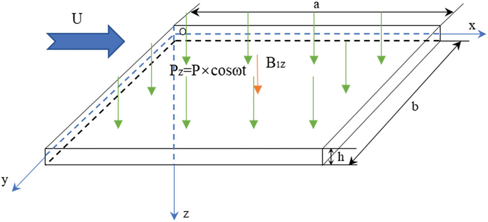
Figure 1: Rectangular conductive thin plate model under the combined action of subsonic airflow and periodic excitation in a magnetic field
The research idea of this paper is shown in Fig. 2 below.
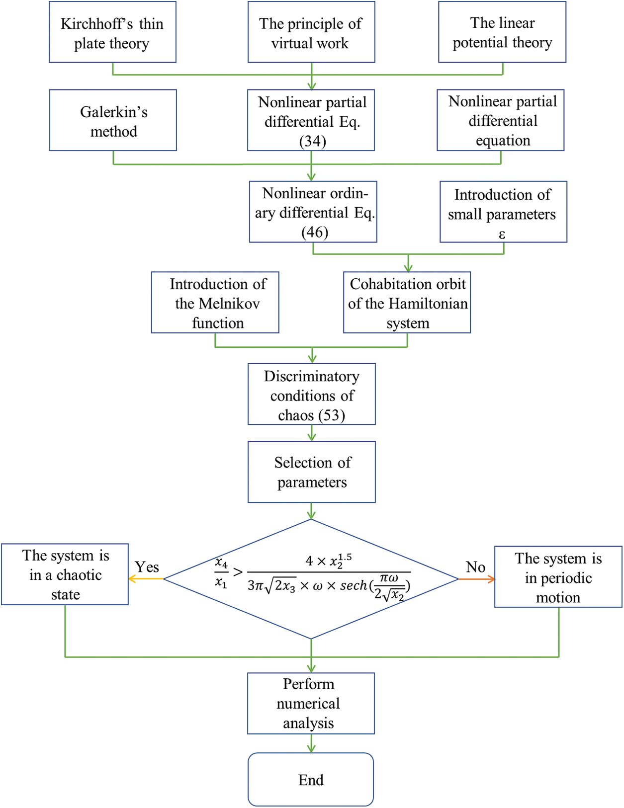
Figure 2: Flow chart of the article’s expository ideas
2.1 Four Basic Conditional Assumptions of Thin Plate Theory
When studying the lateral vibration of elastic thin plates, there are four basic assumptions [30]:
(1) The vertical line segment perpendicular to the mid-plane of the thin plate has no change in its properties and is perpendicular to the deformed mid-plane.
(2) The layers of materials parallel to the middle surface do not have mutual extrusion.
(3) When the plate is bent, the amount of deflection in the z direction changes to zero.
(4) When the plate is bent, there is no expansion and shear deformation at each point in the middle plane of the plate.
2.2 Stress Strain Relationship
According to the elastic deformation theory, when the plate moves, the displacement of each point whose internal distance is z from the mid-plane can be expressed as follows:
In Eq. (1), u, v, w are the displacement components of the points in the midplane, t denotes time, and
According to the assumption of the Kirchhoff straight line method,
In Eq. (2),
where
According to the basic assumption of Kirchhoff, using the generalized Hooke’s law [30], the stress can be described as:
In Eq. (3), E is the Young’s modulus of the material, and μ is the Poisson’s ratio. The equation for large deflection bending of the plate can be obtained as:
In Eqs. (4)–(9),
2.3 Preliminary Establishment of Partial Differential Equations of Motion
During the imaginary displacement, the increment of deformation potential energy of the plate is:
The imaginary work done by the external force on the imaginary displacement is:
According to the principle of virtual displacement, the condition for the system to remain stationary is the external force acting on the system, and the sum of the virtual work done on the virtual displacement and the system deformation potential energy is zero [31], namely:
According to Kirchhoff’s theory, considering the coupling effect of the thin plate under the external excitation and the electromagnetic field, using the principle of virtual work, the following magnetoelastic equation can be obtained as [16]:
In Eqs. (11)–(15),
2.4 Derivation of Basic Theory of Electromagnetic Field
Assuming that the thin plate is a non-polarized, non-magnetized material with good conductivity, the electromagnetic quantity satisfies the Maxwell equation [13]:
The electromagnetic constitutive relation is as follows:
In Eqs. (16) and (17),
When it is in the motion state under the magnetic field, the electromagnetic quantity in the thin plate can be written as:
In Eqs. (18)–(21),
From the Eq. (17), the in-plane induced current can be obtained as:
2.5 Differential Equation of Motion of Rectangular Thin Plate under External Excitation in Transverse Magnetic Field
The vector expression of the Lorenz force acting on a deformed object by an electromagnetic field is:
The unit volume electromagnetic force is:
Integrating Eqs. (26)–(28) in z from
Substituting Eqs. (29)–(33) and the corresponding equation into Eqs. (13)–(15), considering the existence of lateral deformation and damping, the following partial differential equation of motion of a rectangular thin plate in a transverse magnetic field environment can be obtained [15]:
In Eqs. (34)–(36),
From the simply supported condition of the four sides of the rectangular thin plate, the method of separation of variables [22,32] is adopted, and the lateral displacement is given as:
Using the mode shape superposition method, the solution
In the above equations,
According to the linear potential theory [1,33], the pneumatic pressure
Substitute Eqs. (35), (36), (38), (39) into Eq. (34), and use Galerkin’s method to integrate [34], the ordinary differential equation is obtained:
The parameters
Let
The damping coefficient and the force coefficient are considered as perturbation terms. Introducing the small parameter
where
Assuming
Let
A hyperbolic saddle point in the q-z plane and two homoclinic orbits [36]:
3.2 Necessary Conditions for Chaos to Exist
When
The generalized Melnikov function
If the Melnikov function has only one simple zero, the Poincaré map of the disturbance system Eq. (48) has a Strange Attractor, and chaotic motion is possible.
With the continuous increase of
4 Results and Analysis of Example
Numerical simulations are performed using MATLAB software, and the Four-Order Range-Kuttle Method is used for iterative calculations to obtain the bifurcation diagram, phase portrait, Poincaré map and time history response of the system.
The structure and material parameters are selected as:
The surface corresponding to
The motion of the system discussed in this paper is affected by two changing factors, that is, the magnetic field distribution
4.1 When the Magnetic Field Distribution
Selecting
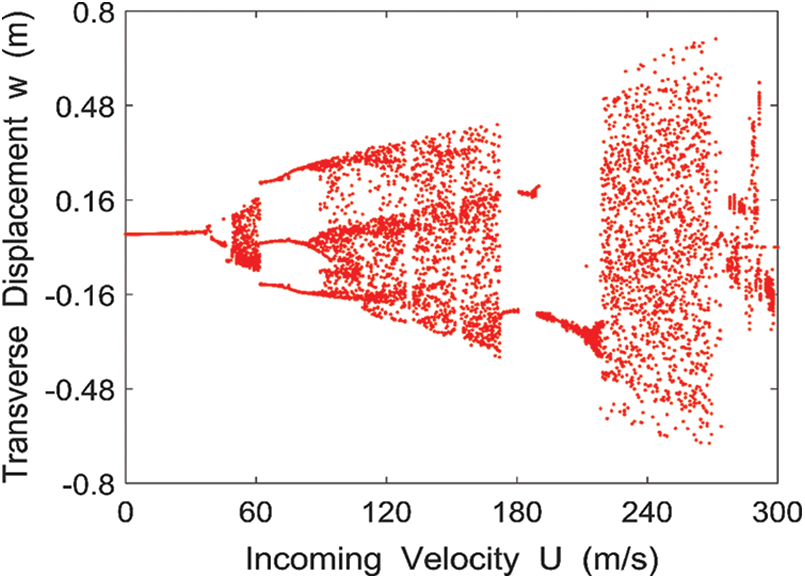
Figure 3: Bifurcation diagram of the lateral displacement of the midpoint of the rectangular conductive thin plate with respect to the incoming velocity
Take
The time history response for the four cases of
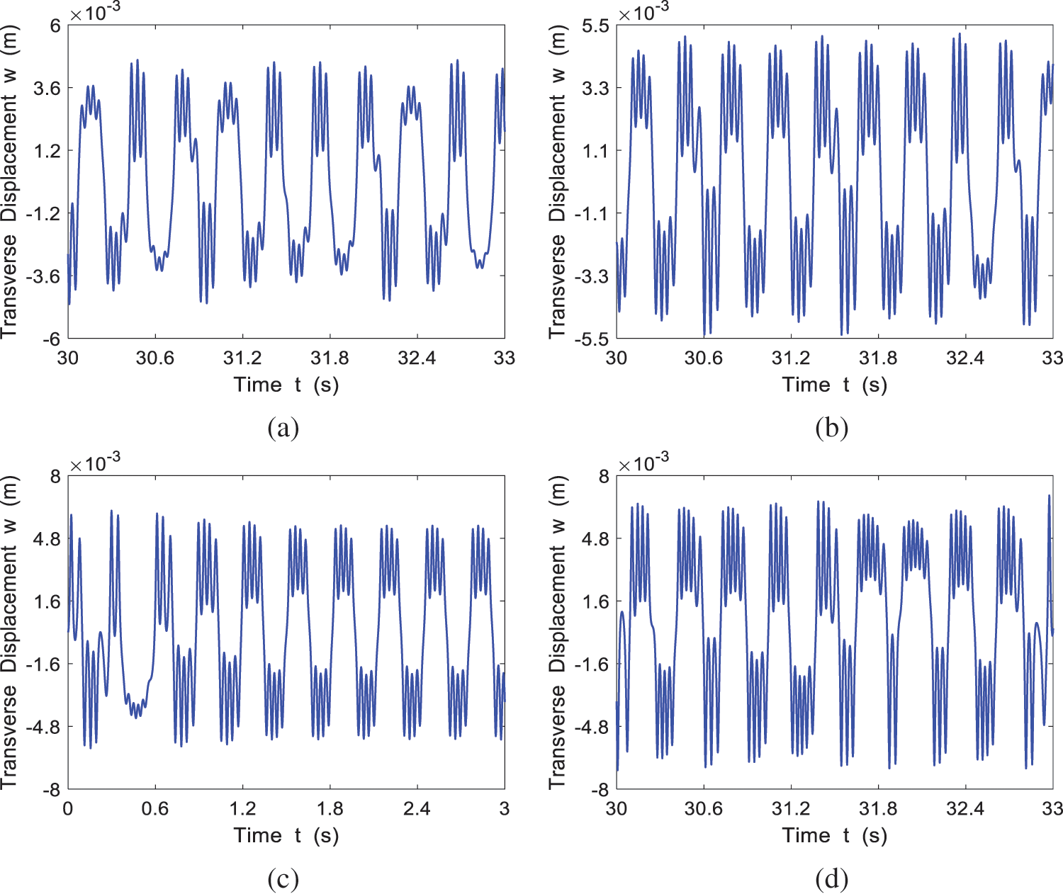
Figure 4: The time history response of the system at different incoming velocities
The phase portrait for the four cases of
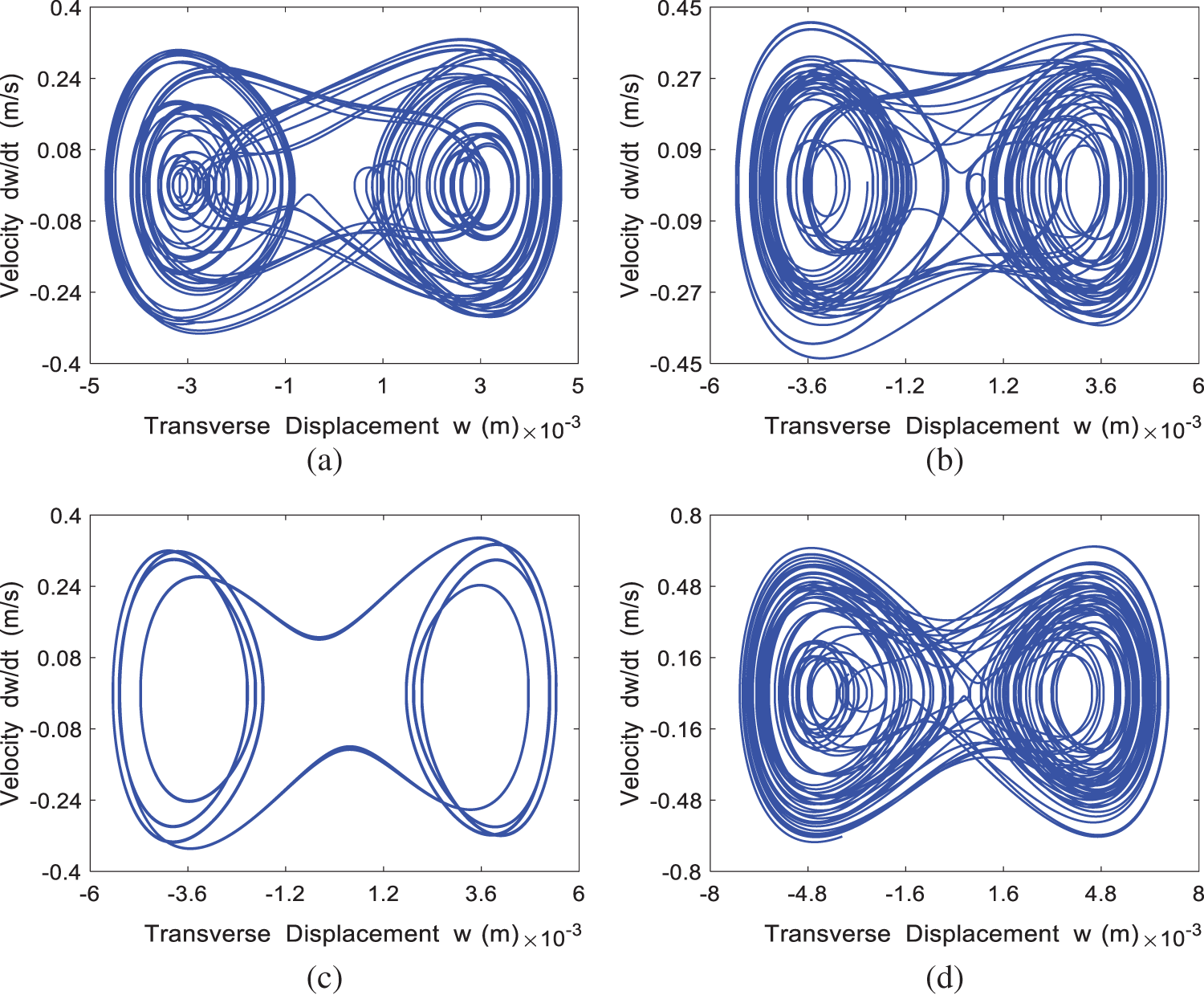
Figure 5: The phase portrait of the system at different incoming velocities
The Poincaré map for the four cases of
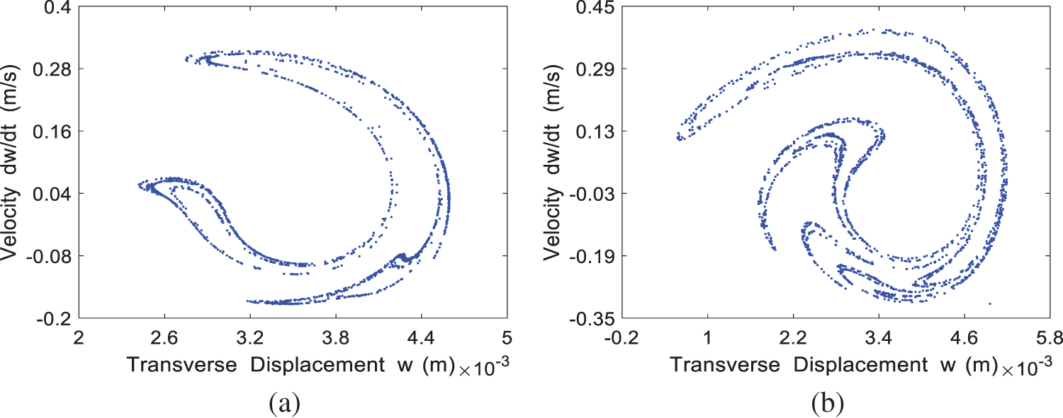
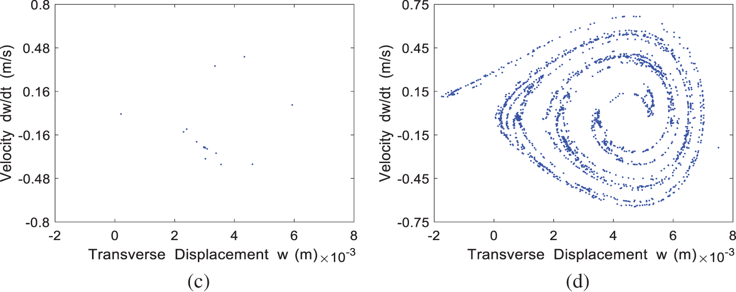
Figure 6: The Poincaré map of the system at different incoming velocities
4.2 When the Magnetic Field Distribution
Selecting
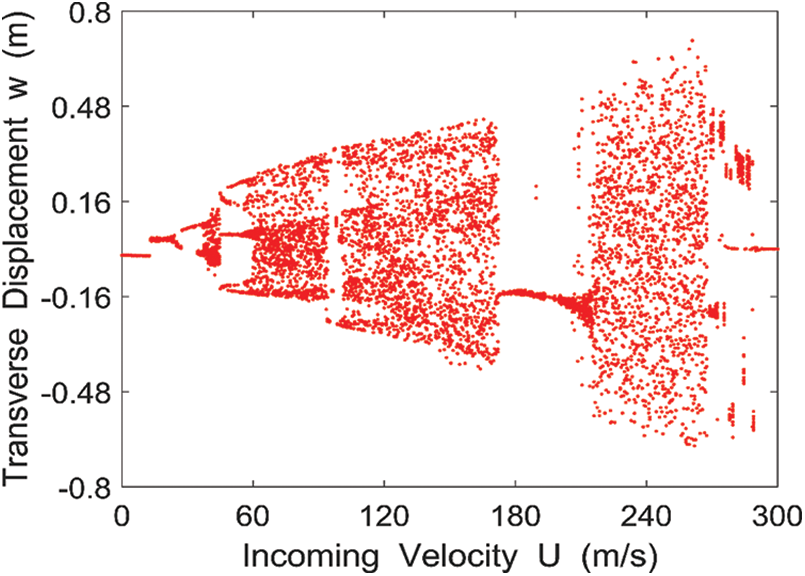
Figure 7: Bifurcation diagram of the lateral displacement of the midpoint of the rectangular conductive thin plate with respect to the incoming velocity
Take
The time history response for the four cases of
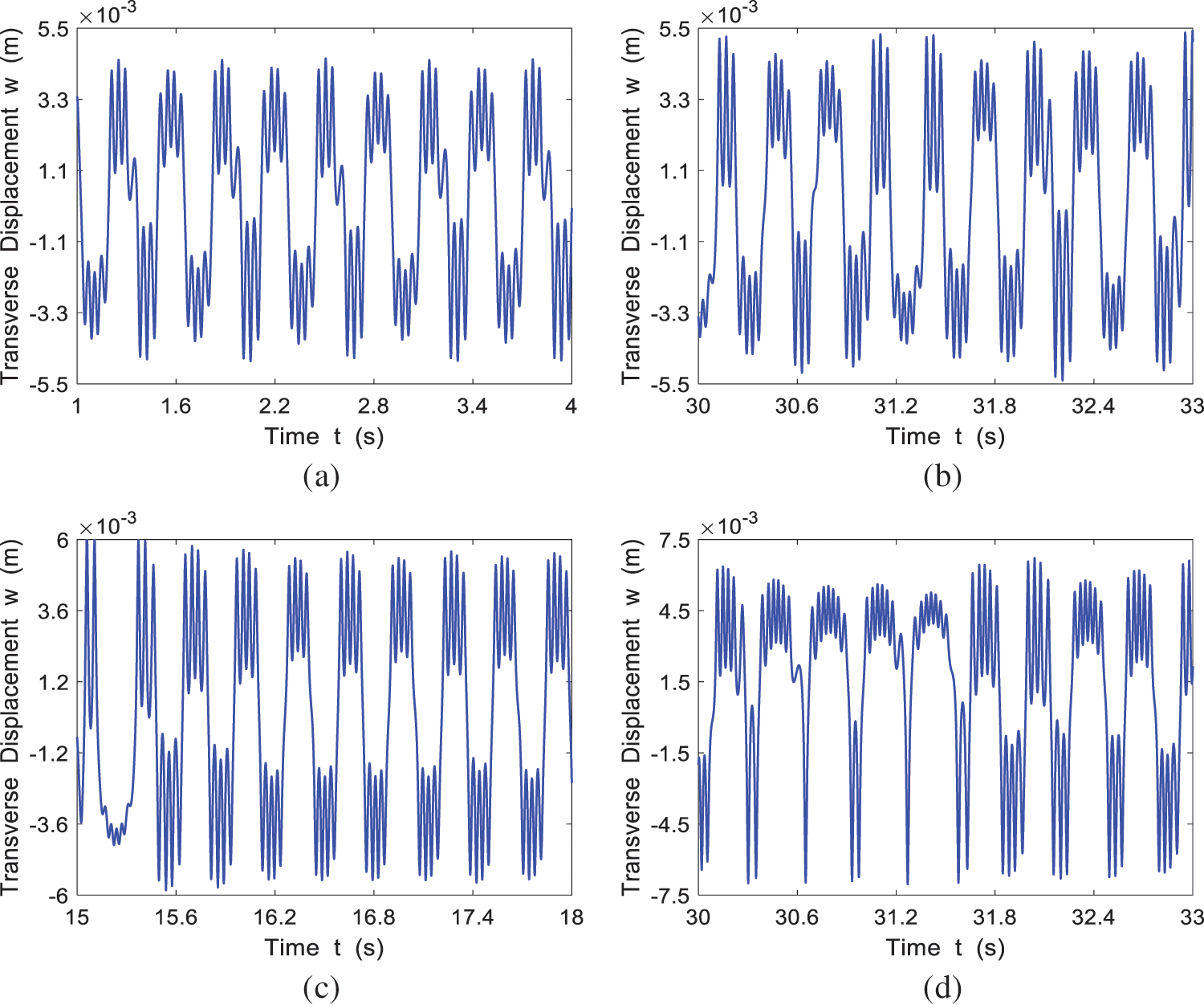
Figure 8: The time history response of the system at different incoming velocities
The phase portrait for the four cases of
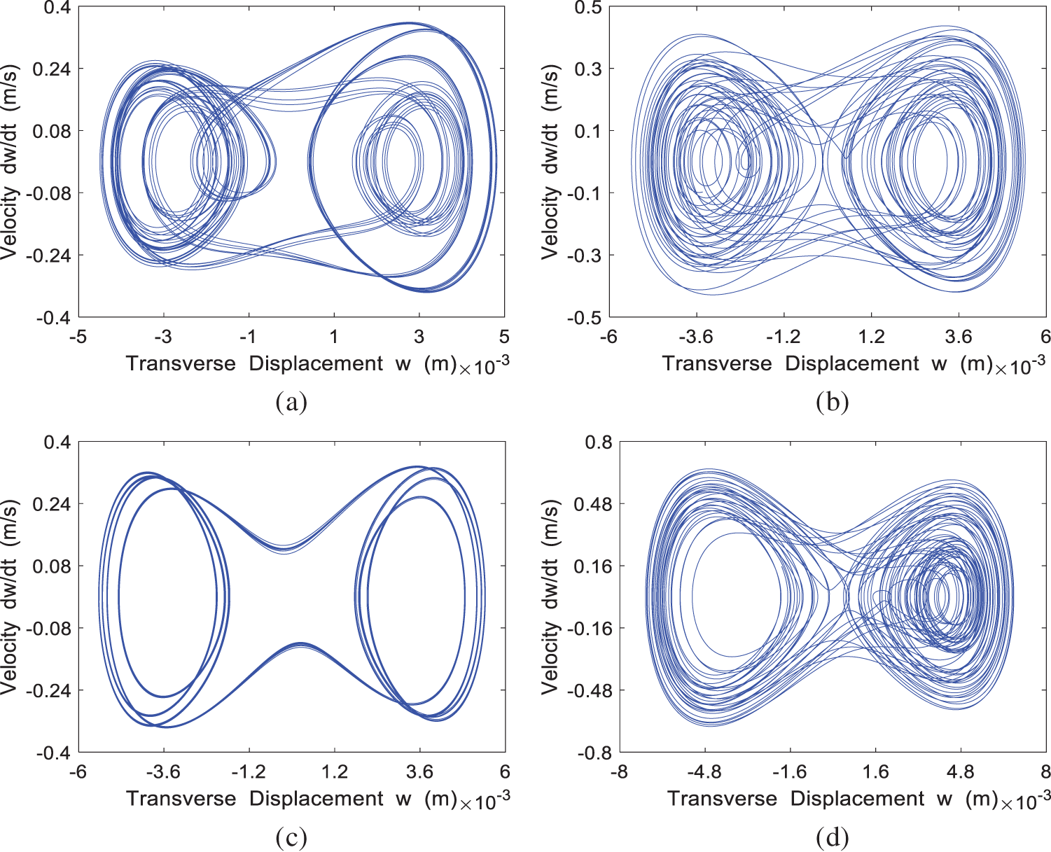
Figure 9: The phase portrait of the system at different incoming velocities
The Poincaré map for the four cases of
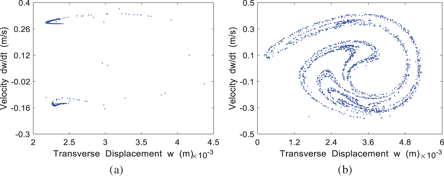
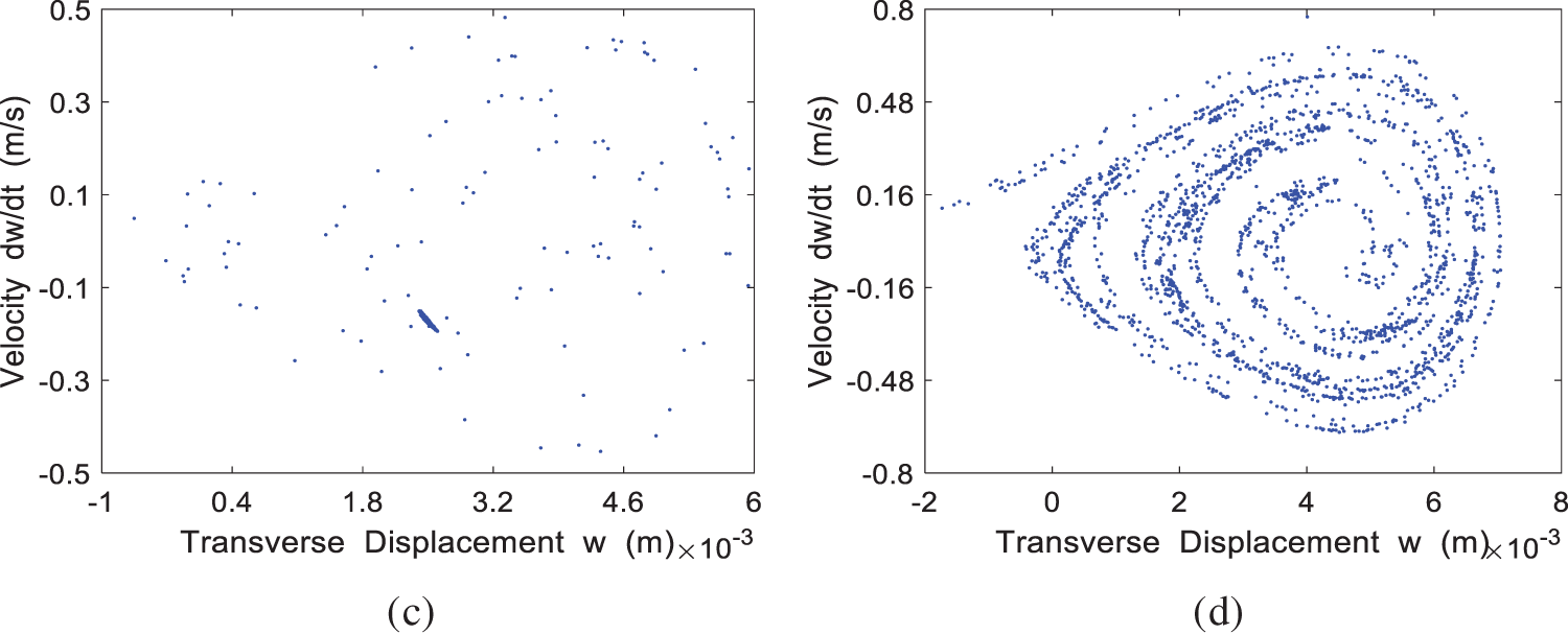
Figure 10: The Poincaré map of the system at different incoming velocities
4.3 When the Magnetic Field Distribution
Selecting
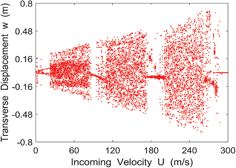
Figure 11: Bifurcation diagram of the lateral displacement of the midpoint of the rectangular conductive thin plate with respect to the incoming velocity
Take
The time-history curve for the four cases of
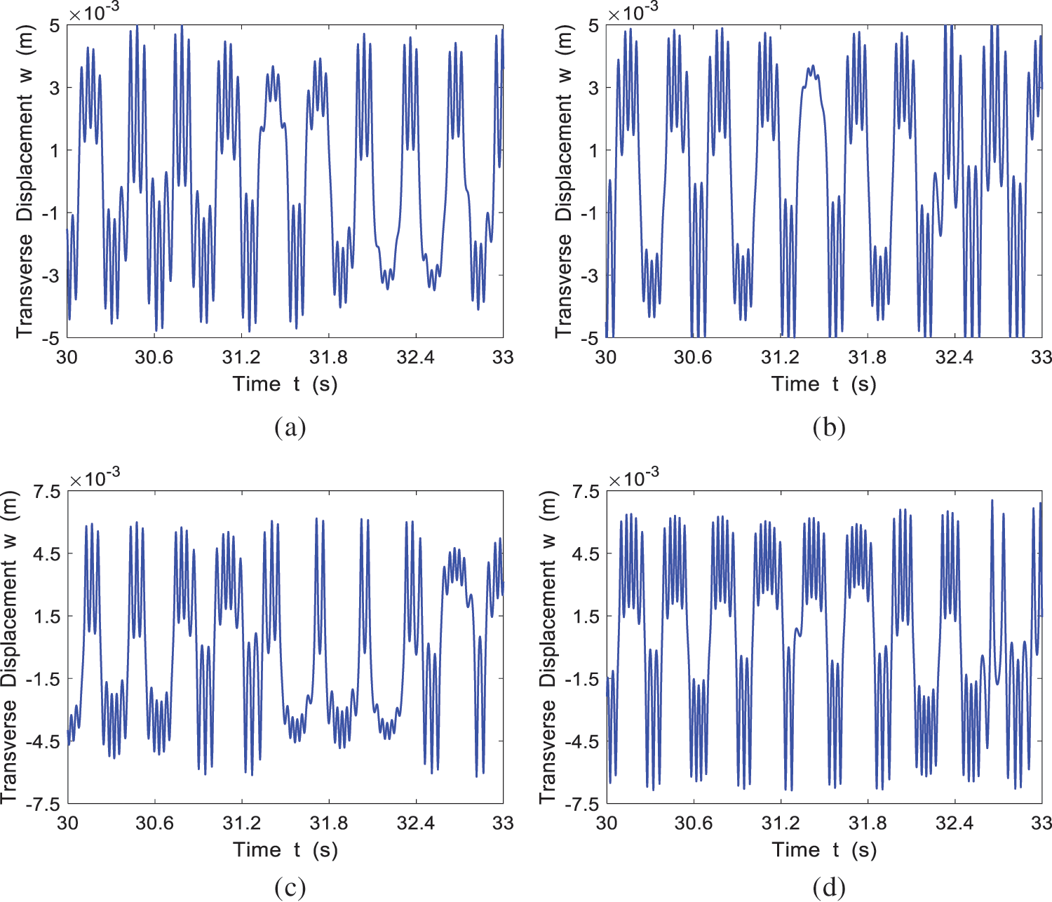
Figure 12: The time history response of the system at different incoming velocities
The phase portrait for the four cases of
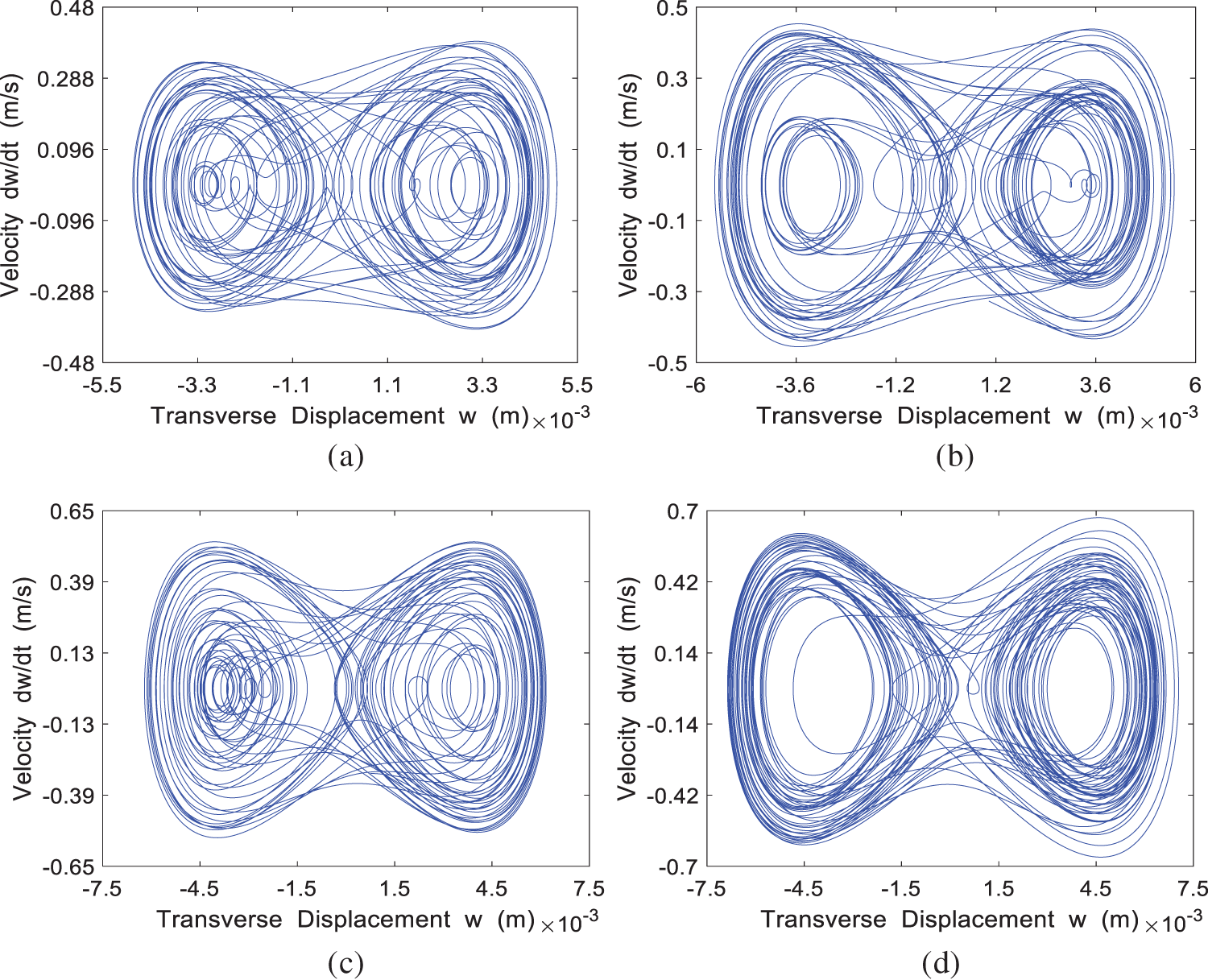
Figure 13: The phase portrait of the system at different incoming velocities
The Poincaré map for the four cases of
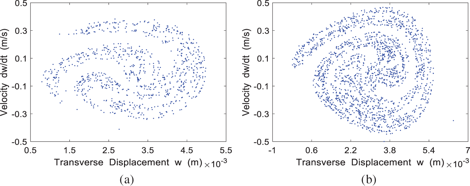
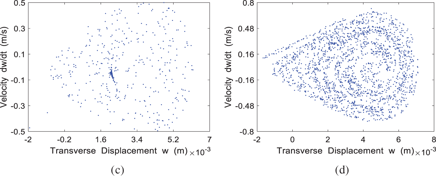
Figure 14: The Poincaré map of the system at different incoming velocities
In this paper, the effects of incoming velocity, magnetic field, and periodic mechanical force on the kinematic behavior of a rectangular conductive thin plate are studied. According to Kirchhoff’s thin plate theory, considering the geometric nonlinearity, the nonlinear dynamic equation of the system motion is established by using the principle of virtual work. The Galerkin’s method is used and the Hamiltonian system is introduced to analyze the Hamiltonian system with Melnikov functions to obtain the criterion for the existence of chaos. The bifurcation diagram, time history response, phase portrait and Poincaré map of the system under different magnetic field strengths are obtained through MATLAB simulation, and the chaotic motion of the rectangular conductive thin plate is qualitatively analyzed. Numerical results verify the possibility of chaotic behavior when the structural parameters given by the theoretical analysis satisfy certain conditions.
(1) Based on the theoretical analysis and numerical calculation results, the chaotic motion is related to the incoming velocity and the magnetic field strength. When
(2) The change of magnetic field only changes the value of
(3) With the constant change of the incoming velocity, the motion of the rectangular conductive thin plate will enter an unstable state, resulting in chaotic motion. The increase of the magnetic field strength
Funding Statement: This research was funded by the Anhui Provincial Natural Science Foundation (Grant No. 2008085QE245), the Natural Science Research Project of Higher Education Institutions in Anhui Province (2022AH040045), the Project of Science and Technology Plan of Department of Housing and Urban-Rural Development of Anhui Province (2021-YF22).
Conflicts of Interest: The authors declare that they have no conflicts of interest to report regarding the present study.
References
1. Dowell, E. H. (1979). Aeroelasticity of plates and shells. ZAMM-Journal of Applied Mathematics and Mechanics, 59(10), 585–585. [Google Scholar]
2. Li, S. B., Hao, X. Y. (2012). Chaotic motion of a functionally graded materials square thin plate. Advanced Materials Research, 1839(531), 593–596. https://doi.org/10.4028/www.scientific.net/AMR.531.593 [Google Scholar] [CrossRef]
3. Abdulrazzaq, M. A., Muhammad, A. K., Kadhim, Z. D., Faleh, N. M. (2020). Vibration analysis of nonlocal strain gradient porous FG composite plates coupled by visco-elastic foundation based on DQM. Coupled Systems Mechanics, 9(3), 201–217. [Google Scholar]
4. Zhang, W., Chen, J. E., Gao, D. X., Chen, L. H. (2014). Nonlinear dynamic responses of a truss core sandwich plate. Composite Structures, 108, 367–386. https://doi.org/10.1016/j.compstruct.2013.09.033 [Google Scholar] [CrossRef]
5. Dugundjim, J., Dowell, E. H., Perkin, B. (1963). Subsonic flutter of panels on continuous elastic foundations. AIAA Journal, 1(5), 1146–1154. https://doi.org/10.2514/3.1738 [Google Scholar] [CrossRef]
6. Tang, M., Tang, J. F., Zhou, D. S., Yu, D. R. (2021). Nonlinearity of initiating and extinguishing boundaries of DBDs with airflows. Plasma Science and Technology, 23(6). https://doi.org/10.1088/2058-6272/abea05 [Google Scholar] [CrossRef]
7. Zhao, K., He, D. W., Fu, S. H., Bai, Z. Y., Miao, Q. et al. (2022). Interfacial coupling and modulation of van der waals heterostructures for nanodevices. Nanomaterials, 12(19), 3418–3418. https://doi.org/10.3390/nano12193418 [Google Scholar] [PubMed] [CrossRef]
8. Kumar, A., Khurana, A., Sharma, A. K., Joglekar, M. M. (2022). Dynamics of pneumatically coupled visco-hyperelastic dielectric elastomer actuators: Theoretical modeling and experimental investigation. European Journal of Mechanics-A/Solids, 95. https://doi.org/10.1016/j.euromechsol.2022.104636 [Google Scholar] [CrossRef]
9. Tang, D. M., Henry, J. K., Dowell, E. H. (1999). Limit cycle oscillations of delta wing models in low subsonic flow. AIAA Journal, 37(11), 1355–1362. https://doi.org/10.2514/2.627 [Google Scholar] [CrossRef]
10. Qiao, Y., Yao, G. (2022). Stability and nonlinear vibration of an axially moving plate interacting with magnetic field and subsonic airflow in a narrow gap. Nonlinear Dynamics, 110(4), 3187–3208. https://doi.org/10.1007/s11071-022-07805-9 [Google Scholar] [CrossRef]
11. Zhang, D. C., Li, P., Zhu, Y. Z., Yang, Y. R. (2022). Aeroelastic instability of an inverted cantilevered plate with cracks in axial subsonic airflow. Applied Mathematical Modelling, 107, 782–801. https://doi.org/10.1016/j.apm.2022.03.019 [Google Scholar] [CrossRef]
12. Ge, G., Zhu, W. Z. (2011). An improved way of detecting the threshold value of chaotic motion on a parametrical excited rectangular thin plate. Applied Mechanics and Materials, 1326(66), 833–837. https://doi.org/10.4028/www.scientific.net/AMM.66-68.833 [Google Scholar] [CrossRef]
13. Hu, Y. D., Li, J. (2008). The magneto-elastic combination resonances analysis of current-conducting thin plate in magnetic field. Journal of Sound and Vibration, 29(8), 1053–1066. [Google Scholar]
14. Hu, Y. D., Li, J. (2008). Nonlinear magneto-elastic vibrating equations and response analysis of a current-conducting thin plate. International Journal of Structural Stability and Dynamics, 8(4), 597–613. https://doi.org/10.1142/S0219455408002855 [Google Scholar] [CrossRef]
15. Li, J., Hu, Y. D., Wang, Y. N. (2017). The magneto-elastic internal resonances of rectangular conductive thin plate with different size ratios. Journal of Mechanics, 34(5), 711–723. https://doi.org/10.1017/jmech.2017.30 [Google Scholar] [CrossRef]
16. Pao, Y. H., Yeh, C. S. (1973). A linear theory for soft ferromagnetic elastic solids. International Journal of Engineering Science, 11(4), 415–436. https://doi.org/10.1016/0020-7225(73)90059-1 [Google Scholar] [CrossRef]
17. Sh, E. L., Kattimani, S., Vinyas, M. (2022). Nonlinear free vibration and transient responses of porous functionally graded magneto-electro-elastic plates. Archives of Civil and Mechanical Engineering, 22(1). https://doi.org/10.1007/s43452-021-00357-6 [Google Scholar] [CrossRef]
18. Chen, J. E., Liu, Y. Q., Liu, W., Su, X. Y. (2013). Themal buckling analysis of truss core sandwich plates. Applied Mathematics and Mechanics, 34(10), 1177–1186. https://doi.org/10.1007/s10483-013-1737-9 [Google Scholar] [CrossRef]
19. Chen, J. E., Zhang, W., Yao, M. H., Liu, J. (2018). Vibration reduction in truss core sandwich plate with internal nonlinear energy sink. Composite Structures, 193, 180–188. https://doi.org/10.1016/j.compstruct.2018.03.048 [Google Scholar] [CrossRef]
20. Agarwal, S., Dash, B., Saini, P., Sharma, N., Mahapatra, T. R. et al. (2020). Vibroacoustic analysis of un-baffled layered composite plate under thermal environment. Materials Today: Proceedings, 24(2), 1020–1028. [Google Scholar]
21. Liu, Y. F., Qin, Z. Y., Chu, F. L. (2022). Investigation of magneto-electro-thermo-mechanical loads on nonlinear forced vibrations of composite cylindrical shells. Communications in Nonlinear Science and Numerical Simulation, 107. https://doi.org/10.1016/j.cnsns.2021.106146 [Google Scholar] [CrossRef]
22. Liu, Y. F., Qin, Z. Y., Chu, F. L. (2021). Nonlinear forced vibrations of functionally graded piezoelectric cylindrical shells under electric-thermo-mechanical loads. International Journal of Mechanical Sciences, 201, 106474. https://doi.org/10.1016/j.ijmecsci.2021.106474 [Google Scholar] [CrossRef]
23. Malikan, M., Eremeyev, V. A. (2022). The effect of shear deformations’ rotary inertia on the vibrating response of multi-physic composite beam-like actuators. Composite Structures, 297, 115951. https://doi.org/10.1016/j.compstruct.2022.115951 [Google Scholar] [CrossRef]
24. Malikan, M., Eremeyev, V. A. (2022). Flexomagneticity in buckled shear deformablehard-magnetic soft structures. Continuum Mechanics and Thermodynamics, 34, 1–16. https://doi.org/10.1007/s00161-021-01034-y [Google Scholar] [CrossRef]
25. Gladkov, S. O. (2021). Theory of electromagnetic radiation by inertially moving conductive bodies. Journal of Communications Technology and Electronics, 66(6), 690–693. https://doi.org/10.1134/S1064226921060115 [Google Scholar] [CrossRef]
26. Zhang, J., Shen, X., Wang, Y., Ji, C., Zhou, Y. et al. (2020). Design of two-dimensional multiferroics with direct polarization-magnetization coupling. Physical Review Letters, 125(1), 017601. https://doi.org/10.1103/PhysRevLett.125.017601 [Google Scholar] [PubMed] [CrossRef]
27. Moon, F. C., Holmes, P. J. (1979). A magnetoelastic strange attractor. Journal of Sound and Vibration, 65(2), 275–296. https://doi.org/10.1016/0022-460X(79)90520-0 [Google Scholar] [CrossRef]
28. Wen, H. H., Duan, Y. H., Pan, L. X. (1997). An analytical study for controlling unstable, periodic motion in magneto-elastic chaos. Physics Letter A, 234(3), 198–204. https://doi.org/10.1016/S0375-9601(97)00501-X [Google Scholar] [CrossRef]
29. Lu, Q. S., To, C. W. S., Huang, K. L. (1995). Dynamic stability and bifurcation of an alternating load and magnetic field excited magnetoelastic beam. Journal of Sound and Vibration, 181(5), 873–891. https://doi.org/10.1006/jsvi.1995.0175 [Google Scholar] [CrossRef]
30. Ershkov, S. V., Leshchenko, D., Giniyatullin, A. R. (2021). A new solving procedure for the kelvin–Kirchhoff equations in case of a falling rotating torus. International Journal of Bifurcation and Chaos, 31(1). https://doi.org/10.1142/S0218127421500103 [Google Scholar] [CrossRef]
31. Ogawa, S., Hamauzu, S., Kikuma, T. (2000). A notion of strain and stress tensor for finite deformation of elastic-plastic continua. Journal of the Society of Materials Science, 49(6), 80–87. https://doi.org/10.2472/jsms.49.6Appendix_80 [Google Scholar] [CrossRef]
32. Sokhal, S., Verma, S. R. (2021). A Fourier wavelet series solution of partial differential equation through the separation of variables method. Applied Mathematics and Computation, 388. https://doi.org/10.1016/j.amc.2020.125480 [Google Scholar] [CrossRef]
33. Li, P., Yang, Y. R., Zhang, M. L. (2011). Melnikov’s method for chaos of a two-dimensional thin panel in subsonic flow with external excitation. Mechanics Research Communications, 38(7), 524–528. https://doi.org/10.1016/j.mechrescom.2011.07.008 [Google Scholar] [CrossRef]
34. Ge, H. X., Zhu, T. (1998). A new meshless local petrov-galerkin (MLPG) approach in computational mechanics. Computational Mechanics, 22, 117–127. https://doi.org/10.1007/s004660050346 [Google Scholar] [CrossRef]
35. Chen, F. F., Qian, D. B. (2022). An extension of the Poincaré-Birkhoff theorem for Hamiltonian systems coupling resonant linear components with twisting components. Journal of Differential Equations, 321, 415–448. https://doi.org/10.1016/j.jde.2022.03.016 [Google Scholar] [CrossRef]
36. Chen, L. Q. (1991). The necessary condition for the appearance of chaos in two classes of forced vibration system with both square and cubic nonlinear terms. Acta Mechanica Solida Sinica, 4(4), 381–386. [Google Scholar]
37. Wiggins, S. (1988). Global bifurcations and chaos. New York: Springer Verlag. [Google Scholar]
38. Wiggins, S. (1990). Introduction to applied nonlinear dynamical systems and chaos. New York: Springer Verlag. [Google Scholar]
39. Feng, J. H., Li, Y. (2021). The weak smale horseshoe and mean hyperbolicity. Journal of Differential Equations, 299, 154–195. https://doi.org/10.1016/j.jde.2021.07.020 [Google Scholar] [CrossRef]
Cite This Article
 Copyright © 2023 The Author(s). Published by Tech Science Press.
This work is licensed under a Creative Commons Attribution 4.0 International License , which permits unrestricted use, distribution, and reproduction in any medium, provided the original work is properly cited.
 Downloads
 Citation Tools