Transductive Transfer Dictionary Learning Algorithm for Remote Sensing Image Classification

1  Introduction

The ecological environment is closely related to human life. A good ecological environment is the foundation of human survival and health. At present, maintaining a healthy ecological environment has been the consensus of people all over the world. Ecological environment monitoring refers to the monitoring activities carried out to accurately, timely, and comprehensively reflect the ecological environment status and its changing trend with the objects of mountains, water, forests, fields, lakes, and grasses. The rapid development of satellite and aviation technology makes the application of remote sensing technology an important part of ecological environmental monitoring [1]. A large amount of real-time and reliable ecological environmental image information can be obtained by using satellite remote sensing images. Remote sensing image classification is the process of real-time scene classification and recognition based on the content extracted from images. Improving the accuracy of scene image classification can bring many conveniences to ecological environmental monitoring. Remote sensing image classification labels an image as a high-level semantic class [2]. Different from pixel-based semantic segmentation, it only pays attention to which pixels correspond to a certain feature. In scene classification, a small-scale image has its semantic information and can be classified into a certain semantic class through semantic features. Therefore, the overall cognition of a remote sensing image constitutes the scene class. The texture and spatial features of a scene, as well as the relationship between the objects, enable not only to describe the underlying physical features of the image, but also to characterize the semantic information of images. Dictionary learning has achieved success in this field due to its sparse representation and reconstruction capabilities. For example, Soltani-Farani et al. [3] developed a spectral and contextual characteristics-based dictionary learning algorithm for multispectral resolution sample classification. The linear combinations of two features of spectral are used as the common elements in the dictionary. Vu et al. [4] developed a dictionary learning model characterized by shared and class-specific dictionaries. Especially, the Fisher discrimination and low-rank constraints are enforced for the learned dictionaries. Geng et al. [5] used an online dictionary learning algorithm with the special atom’s selection strategy. The particle swarm optimization algorithm was adopted in the model update phase.

In scene classification, some different scene classes may contain similar feature representations and spatial texture structures [6]. For example, commercial and residential areas often contain houses, vehicles, highways, and interchanges. Bridges often contain roads, vehicles, and other objects. There will also be large differences in characteristics in the same class of scene, such as parking lots with cars and parking lots without cars. Thus, how to effectively and efficiently classify scenes is a challenging problem. In addition, nature scenes are rich and diverse, and even the same ground object may exhibit different characteristics under different time and space conditions, which results in “the same object with different spectrum” and “different objects with the same spectrum”. Such differences make most remote sensing application fields lack suitable labeled sample sets. At present, most remote sensing image processing problems based on artificial intelligence adopt supervised learning algorithms. The supervised learning algorithms require sufficiently fine-grained data labeling of the target image, and use these manually labeled remote sensing samples to train effective automatic classifiers on data with the same feature distribution. Therefore, it is a challenge to utilize traditional supervised learning algorithms to build a universal and reusable remote sensing image processing model [7].

Transfer learning is a type of algorithm of using the relevant dataset (called source domain) to calibrate the target domain when the source domain with sufficient class labels and the target domain with insufficient labels (or without class labels) have different feature distributions [8]. In practical applications, a large number of pre-labeled images or open-source public datasets are readily available, which can be used as the source domain. Due to the difference in objective factors such as sensors, algorithms, atmospheric conditions, solar radiation, ground features, building styles, and vegetation characteristics of data acquisition, there are often differences between different domains. To solve this problem, Zhou et al. [9] proposed the correlation alignment (CORAL) algorithm to achieve domain adaptation and capture the texture of the image structure. Tuia et al. [10] developed the spectral feature alignment (SFA) algorithm to use singular value decomposition for calculating the mapping function of feature representation so that the two domains can learn common features independent of their respective domains in a common latent space. Wang et al. [11] developed the structural correspondence learning algorithm to model the correlation of features.

In this paper, we propose a transductive transfer dictionary learning (TTDL) algorithm for remote sensing image classification. By TTDL, the source and target domains are transformed into a common subspace, and the samples in the two domains are re-encoded to have similar feature distributions. In this subspace, a shared dictionary is trained to establish the association between two domains and obtain the sparse representations of two domain samples. Also, the triplet-induced ordinal locality preserving term on subspace projection, Fisher discriminant term on dictionary and graph Laplacian regularization term on sparse representation are introduced into the TTDL algorithm. The triplet-induced ordinal locality preserving term considers the ranking information of each sample’s neighborhood, so it can more accurately describe the local geometry of the data. Fisher’s criterion directly constrains the intra-class distance and inter-class distance of the learned dictionary, instead of constraining the sparse representation. Its direct benefit is that the dictionary atoms of the same class can be more compact, so the similarity between different classes can be greatly reduced and the reconstruction ability and discriminative ability of the dictionary can be enhanced. Following the principle that the sparse representation of the same class should be as similar as possible and the sparse representation of different classes should be as different as possible, the graph Laplacian regularization term on sparse representation is constructed. The semi-supervised weight graph matrix in the source domain is built using the known class labels. Since the weight graph matrix in the target domain is unknown, it appears as a variable in the model optimization and reaches its optimal solution when the algorithm converges. Finally, TTDL obtains the discriminative dictionary and sparse representation, to better complete the remote sensing image classification across datasets.

The contributions of this paper are as follows:

(1) A remote sensing image classification algorithm for cross dataset transfer learning is proposed. Different domains are projected into the subspace to eliminate distribution differences. And the shared dictionary is established the relationship between two domains.

(2) Fisher’s criterion on dictionary improves the intra-class compactness and inter-class differences of sub-dictionary. In this way, one sub-dictionary reconstructs a certain class of training samples, which can enhance the discrimination of the dictionary.

(3) The unsupervised triplet graph in the triplet-induced ordinal locality preserving term is used to exploit the data local structure information. The semi-supervised weight graph matrix is used to maintain the manifold structure. Thereby, the discriminative ability of subspace and sparse representation can be enhanced.

2  Related Work

2.1 Dictionary Learning

Let Y∈Rn×N represent the training data set containing N samples of C classes, where the dimension of samples is n. The dictionary learning [12] is constructed as,

minD,A‖Y−DA‖22+λ‖A‖p,(1)

where D∈Rn×K and A∈RK×N are the dictionary and sparse representation on Y, respectively. ‖Y−DA‖22 represents the reconstruction error term. ‖A‖p represents the regularization constraint of ℓp-norm of sparse representation A. λ>0 is the trade-off parameter. Eq. (1) is not a convex optimal solution. D and A can be solved by an alternate iterative strategy.

In classification tasks, the new test sample ynew can be classified by,

identity(ynew)=arg\,minl‖ynew−Dσl(anew)‖2,(2)

The function σl(anew) returns a vector, whose internal non-zero elements are related to the class of data.

2.2 Fisher Discrimination Dictionary Learning

Fisher discrimination dictionary learning (FDDL) [13] algorithm aims to obtain a structured dictionary of training data. Using Fisher’s criterion, the learned sparse representations belonging to different classes have a large spatial distance, while the sparse representations belonging to the same class have a small spatial distance. The objective function of FDDL is,

minD,A12∑l=1Cr(Yl,D,Al)+λ1‖S‖1+λ22g(A),(3)

where r(Yl,D,Al) is the structure dictionary term. Yl and Al are the class label and sparse representation of the l-th class, respectively. g(A) is the Fisher’s criterion term on sparse representation. r(Yl,D,Al) and g(A) are defined as,

r(Yl,D,Al)=‖Yl−DAl‖F2+‖Yl−DAl‖F2+∑j≠l‖DjAlj‖F2,(4)

g(A)=∑l=1C(∑j=1Nj‖alj−ml‖22−Nl‖ml−m‖F2)+‖A‖F2,(5)

where Dj is the j-th class sub-dictionary. Alj is the sparse representation of Al over Dj. ml and m are the mean vector of Al and A, respectively.

3  Transductive Transfer Dictionary Learning Algorithm

3.1 Objective Function

Let Ys=[y1s,y2s,…,yNss]∈Rn×Ns and Yt=[y1t,y2t,…,yNtt]∈Rn×Nt are the source and target domains, respectively, where Ns and Nt are the size of samples in the source and target domains, respectively, N=Ns+Nt. TTDL uses the orthographic projection matrices Ps∈Rm×n and Pt∈Rm×n(m<n) to project the source and target domains into the low-dimensional common subspace, respectively. The samples of two domains are re-encoded with the same or similar feature distributions in the subspace. Meanwhile, TTDL trains a discriminative dictionary D of domain-invariant features under the framework of dictionary learning, and also obtains the sparse representation As and At for the source and target domains, respectively. Let Y~=[Ys00Yt], P~=[Ps,Pt], A~=[As,At], the objective function of TTDL is represented by,

minP~,A~,D,Qt‖P~Y~−DA~‖F2+θ1‖A~‖F2+θ2Φ(P~)+θ3Z (D)+θ4Γ(A~,Qt),(6)

where Qt is the weight graph matrix in the target domain. Through P~, different domain data is projected into the subspace to eliminate the distribution difference between two domains. Also the shared dictionary D is established the association between two domains. Φ(P~), Z (D) and Γ(A~,Qt) are functions on variables P~, D, A~ and Qt, respectively, which helps to establish the relationship between two domains and improve the discriminative ability of dictionary learning. θ1, θ2, θ3 and θ4 are trade-off parameters, to coordinate the functions of each item in the objective function.

Φ(P~) is the triplet-induced ordinal locality preserving term on projection matrix. We think that the samples in the low dimensional subspace should keep their local structure information in the original space. Φ(P~) considers the ranking information of samples’ neighborhood, so it can more accurately describe the local geometric structure of data. First, we construct the k-nearest neighbor set ϖi for each sample y~i. The sample y~i with two neighbors y~u and y~l builds a triplet (y~i,y~u,y~l). We build the asymmetric distance matrix Ci for y~i, and its element Culi is computed as Culi=‖y~i−y~u‖22−‖y~i−y~l‖22. Then we build the similarity matrix G∈RN×N as,

gil={∑u∈ΩiCuli,l∈ϖi0,l∉ϖi(7)

The triplet-induced ordinal locality preserving term Φ(P~) is represented as,

minP~∑i=1N∑l=1Ngil‖P~Ty~i−P~Ty~l‖2,s.t.P~P~T=I,(8)

Denote Δ∈RN×N is the Laplacian matrix Δ=M−G+GT2. M is the diagonal matrix, where

Mii=∑lgil+gli2.(9)

Eq. (8) can be represented as,

minP~Tr(P~Y~ΔY~TP~T),s.t.P~P~T=I.(10)

Z (D) is the Fisher discriminant term on dictionary. To ensure the dictionary atoms have intra-class compactness and inter-class differences, we implement Fisher discriminant criteria on the dictionary D. Z (D) is represented as,

Z (D)=Tr(Ωw(D)−ΩB(D)).(11)

where Ωw(D) and ΩB(D) are the intra-class scatter and the inter-class scatter on D, respectively,

Ωw(D)=∑l=1C(Dl−D~l)(Dl−D~l)T,(12)

ΩB(D)=∑l=1CKl(Dl−D~)(Dl−D~)T,(13)

where Kl is the number of the lth class atoms. D~ and D~l are the mean values of D and Dl, respectively.

Let El=1Kl1KlT∈RKl×Kl, E=1K1KT∈RK×K, we have D~l=DlEl/Kl,D~=DE/K, Ωw(D) and ΩB(D) can be written as,

Ωw(D)=∑l=1C(DlDlT−1KlDlElDlT),(14)

ΩB(D)=∑l=1CKl(D~lD~lT−2D~lD~T+D~D~T).(15)

Substituting Eqs. (14) and (15) into Eq. (11), Z (D) is represented as,

Z (D)=Tr(DBDT),(16)

where B=IK−Diag(2K1E 1,2K2E 2,…,2KCE C)+1KE .

Γ(S~,Qt) is the graph Laplacian regularization term on sparse representation. We think that the sparse representation of the same class should be as similar as possible, and the sparse representation of different classes should be as different as possible. The weight graph matrix Qs is built on the source domain Ys. The element qijs in Qs is defined as,

qijs={1,yisandyisareofthesameclass0,otherwise(17)

Because the class label of Yt is unknown, TTDL estimates the weight graph matrix Qt in the target domain. Γ(A~,Qt) is represented as,

minA~,Qt∑i=1Ns∑j=1Nsqijs‖a~is−a~js‖2+∑i=1Nt∑j=1Ntqijt‖a~it−a~jt‖2+δ‖Qt‖F2,s.t.qit1=1,qijt≥0(18)

where δ is the trade-off parameter. Let L∈RN×N be the Laplacian matrix with L=W−Q~, Q~=[Qs00Qt] and W be the diagonal matrix with Wii=∑jqij.

minA~,QtTr(A~LA~T)+δ‖Qt‖F2,s.t.qijt1=1,qijt≥0(19)

Combining Eqs. (8), (11), and (19) into Eq. (6), the objective function of TTDL is re-written as,

minP~,A~,D,Qt‖P~Y~−DA~‖F2+θ1‖A~‖F2+θ2Tr(P~Y~ΔY~TP~T)+θ3Tr(DBDT)+θ4Tr(A~LA~T)+δ‖Qt‖F2,s.t.P~P~T=I,qijt1=1,qijt≥0,‖dk‖22≤1,∀k(20)

3.2 Optimization

For the objective function of the TTDL algorithm, four variables P~, A~, D and Qt should be optimized. We adopt the alternately optimization strategy and have the following four steps:

(1) P~ is optimized by fixing A~, D and Qt,

minP~‖P~Y~−DA~‖F2+θ2Tr(P~Y~ΔY~TP~T),s.t.P~P~T=I,(21)

According to [14], there exists the matrices R~∈RN×m, Z∈RN×K, which has the following form: P~=(Y~R~)T, D=P~Y~Z, and K~=Y~TY~. Then we have,

minR~‖R~TK~(I−ZA~)‖F2+θ2Tr(R~TK~ΔK~TR~),s.t.R~TK~R~=I.(22)

We have the closed-form solution of R~ as,

R~=τΣ−1/2σ,(23)

where K~=τΣτT. σ is obtained by,

minσTr(σTHσ),s.t.σTσ=I,(24)

where H=Σ1/2τT((I−ZA~)(I−ZA~)T+θ2ΔτΣ1/2). Obviously, σ has the closed-form solution.

(2) D can be optimized by fixing P~, A~ and Qt,

minD‖P~Y~−DA~‖F2+θ3Tr(DBDT),s.t.‖dk‖22≤1,∀k.(25)

Using the Lagrange dual approach, D is obtained by,

D=P~Y~A~T(A~A~T+θ3B)−1.(26)

(3) S~ is optimized by fixing P~, D and Qt,

minA~‖P~Y~−DA~‖F2+θ1‖A~‖F2+θ4Tr(A~LA~T).(27)

We re-write Eq. (27) in terms of the row vector a~i in A~ as,

mina~i‖(P~Y~)i−Da~i‖22+θ1‖a~i‖22+θ4∑jqi,j‖a~i−a~j‖22.(28)

The closed-form solution of a~i is,

a~i=(DTD+θ4∑jqi,jI+θ1I)−1(DT(P~Y~)i+θ4∑jqi,ja~j).(29)

(4) Qt can be optimized by fixing P~, D and A~, we have,

minQtθ4∑i=1Nt∑j=1Ntqijt‖a~it−a~jt‖2+δ‖Qt‖F2,s.t.qijt1=1,qijt≥0,(30)

We define hi,j=θ4‖a~t,i−a~t,j‖222δ, Eq. (30) is represented as,

minqijt‖qit+hi‖22,s.t.qit1=1,qijt≥0,∀i,j(31)

The closed-form solution of qit is,

qit=(1+∑j=1kh^ijk1−hi)+,(32)

where (⋅)+ means the elements in qit are nonnegative. The element h^ij of h^i is the same as that in hi with the ascending order.

It is noted that according to [14], δ can be computed by,

δ=1Nt∑i=1Nt(k2h^ik+1−12∑j=1kh^ij).(33)

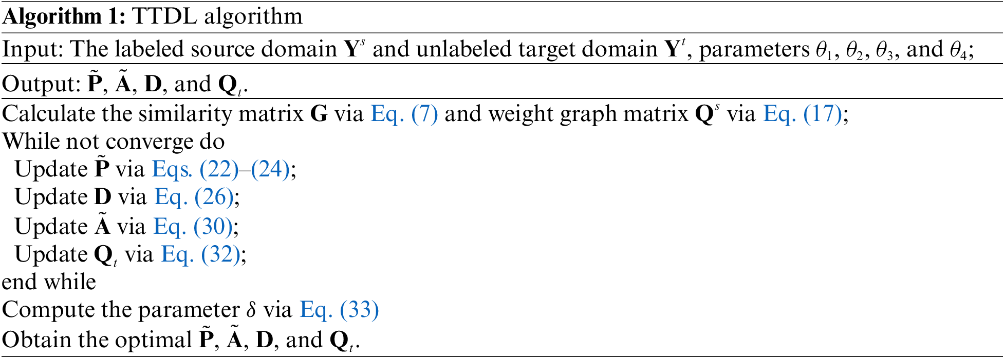
The solving procedure of Eq. (20) is summarized in Algorithm 1.

4  Experiments

4.1 Datasets

The TTDL algorithm is evaluated on real-world remote sensing datasets: RSSCN7 [1], Ucmerced land [2], Aerial image dataset (AID) [15], and SIRI-WHU dataset [16]. The RSSCN7 dataset consists of 2800 images of seven scene classes. There are 400 images of each class, in which the size of each image is 400 × 400 pixels. The Ucmerced land dataset consists of 2100 aerial scene images from 21 classes, with the size of 256 × 256 pixels. The AID dataset is a large scale aerial scene dataset, which consists of 10,000 remote sensing scene images of 30 classes, with the size of 600 × 600 pixels. The SIRI-WHU dataset is also an aerial scene dataset, composed of 12 classes of aerial scene images, in which each class contains 200 images, with the size of 200 × 200 pixels. To efficiently represent the remote sensing images, we adopt two different types of deep feature representations: ResNet50 and VGG-VD-16 [7]. They are extracted by the two convolution neural networks (CNN). The dimensions of the two deep features are 2048.

In the experiment, we design three cross-domain remote sensing image scene classification tasks: Ucmerced→RSSCN7 (named U→R), AID→RSSCN7 (named A→R), and SIRI-WHU→RSSCN7 (named S→R), referring to Ys→Yt. To match the classes in RSSCN7, we select corresponding similar classes to form the source domain, the detailed information of three cross-dataset scene classification tasks is shown in Table 1. Following the ID sequence in Table 1, some sample images of corresponding classes in four remote sensing image datasets are shown in Fig. 1. In the experiments, we randomly select 80% of the images in Ys and 5% of the images in Yt for model training, and the rest of images in Yt are used for testing. Comparison algorithms include: sparse representation-based nearest neighbor (SRNN) [17], maximum mean discrepancy (MMD) [18], generalized joint distribution adaptation (G-JDA) [19], and maximum independence domain adaptation (MIDA) [20], and transfer independently together (TIT) [21]. SRNN is a basic sparse representation algorithm, while MMD, G-JDA, MIDA, and TIT are transfer learning algorithms. The regularization and kernel parameters are set in {2−6,2−5,…,26}. The TTDL algorithm involves four parameters, which are set in {10−3,10−2,…,103}. The size of the sub-dictionary is the same as the number of training images in each class. The experiment is repeated ten times, with each run’s classification accuracy being recorded.

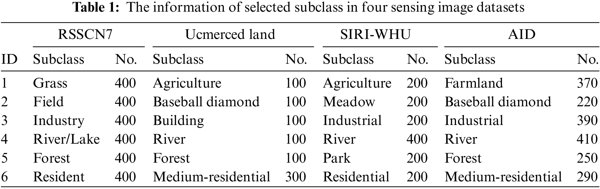
Figure 1: Sample images in four dataset, (a) RSSCN7, (b) Ucmerced land, (c) SIRI-WHU, (d) AID

4.2 Performance Comparison

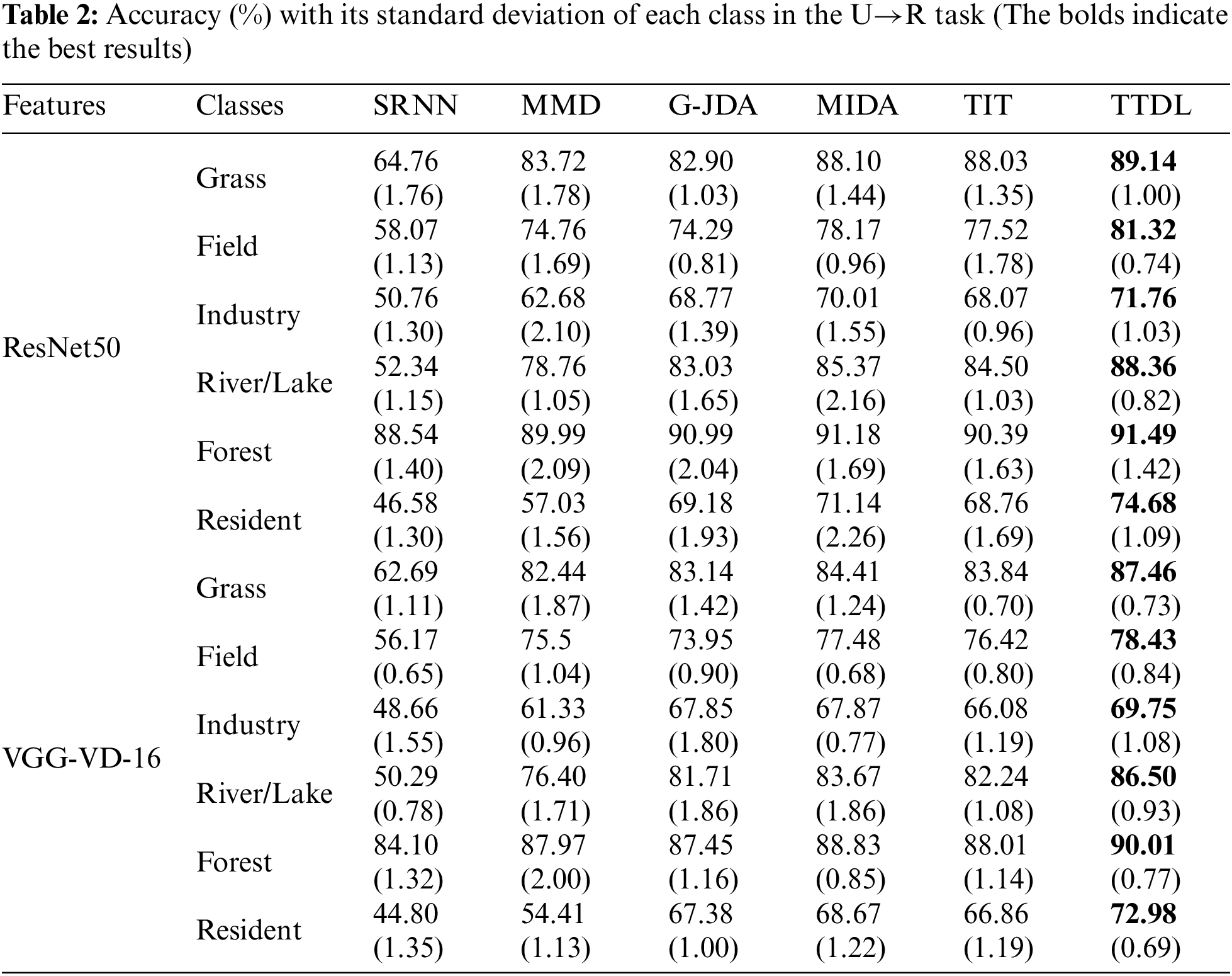
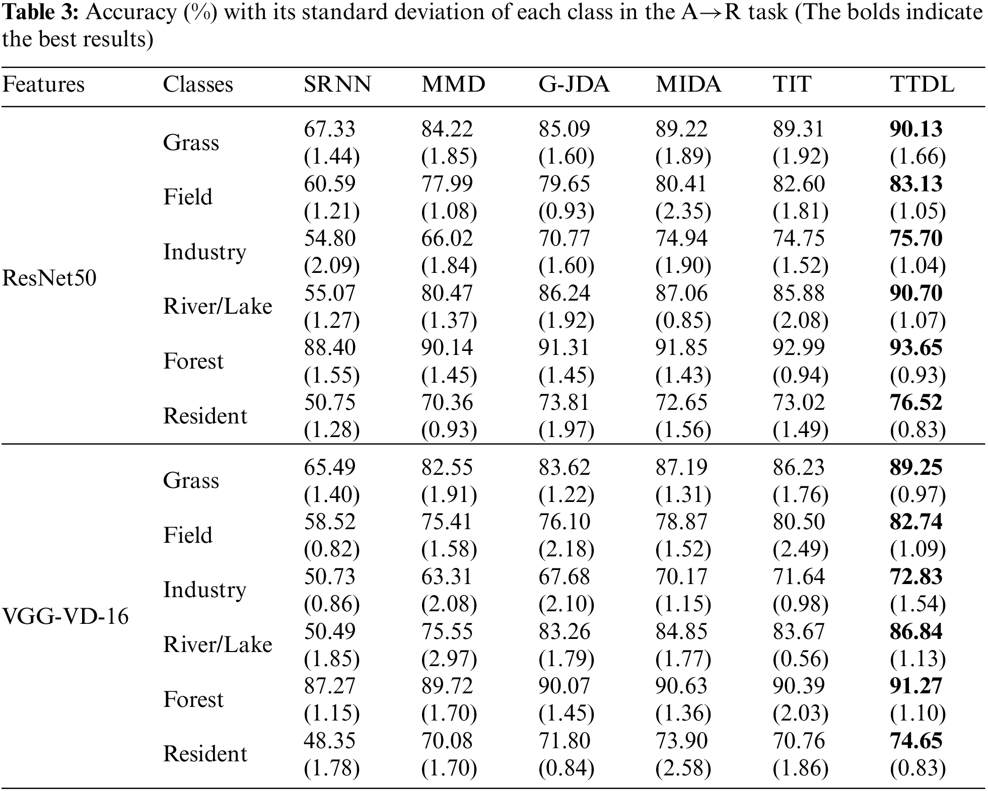
We compare the TTDL algorithm on three cross-domain remote sensing image classification tasks. The accuracy results in each class are shown in Tables 2–4. Analyzing the experimental results, we can see that the TTDL algorithm achieves the best classification accuracy. The baseline algorithm SRNN cannot obtain satisfactory performance in all cross-domain remote sensing image classification tasks. Since SRNN is only trained on the source domain, it cannot be used directly on the RSSCN7 dataset due to differences in data distribution across different domains. G-JDA aligns cross-domain edge feature probability distributions and conditional feature probability distributions in the new feature space by applying their respective projection matrices. TIT also uses landmarks to select representative samples for cross-domain feature matching while maintaining the manifold structure using graphs. Both MMD and MIDA project different domains into the common subspace to achieve cross-domain feature alignment. The above algorithms except TTDL do not consider triplet-induced ordinal locality preserving term, Fisher discriminant term, and graph Laplacian regularization term in transfer learning. The TTDL algorithm not only maintains the local structure in the subspace, but also makes similar sparse representations as similar as possible, to enhance the discriminative performance of sparse representations. Additionally, TTDL minimizes the intra-class scatter of atoms and maximizes the inter-class scatter of atoms, which can greatly promote the discriminative performance of the dictionary.

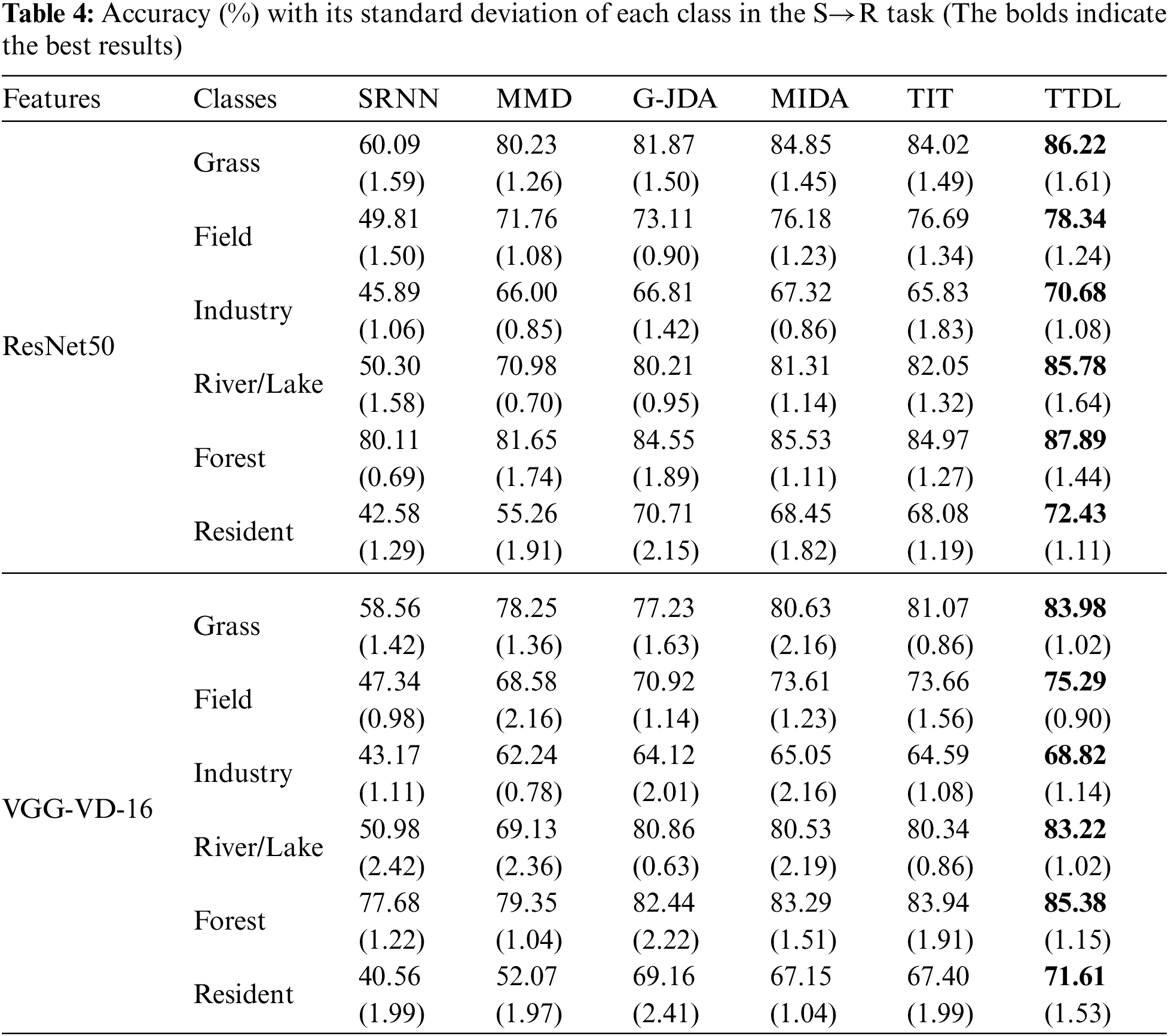
The classification results using ResNet50 and VGG-VD-16 features are comparable. As we know, the contained information in remote sensing scene images is often closely related to its class. The traditional feature information such as color, texture, space, and spectral information is insufficient for remote sensing images. Especially when the features corresponding to some classes are not significant enough, the accuracy of the classifier will be reduced. Thus, the deep features are effective in our experiments.

Fig. 2 records the classification performance of each algorithm in three transfer learning tasks. We can see that the average accuracy of TTDL is the highest among all sub-classes. For example, in the U→R task, using the ResNet50 features, the average accuracy of TTDL is 22.62% higher than the SRNN algorithm, and 3.25% higher than the second best. In the A→R task, using the VGG-VD-16 features, the average accuracy of TTDL is 22.17% higher than the SRNN algorithm, and 1.88% higher than the MIDA algorithm. In the S→R task, using the ResNet50 features, the average accuracy of TTDL algorithm is 25.53% higher than the SRNN algorithm, and 3.28% higher than the second best. These results show that TTDL is effective in three classification tasks of U→R, A→R, and S→R. Thus, the dictionary learning framework combined with subspace learning, Fisher discriminant, and local information preserving is a good choice for cross-dataset remote sensing image classification.

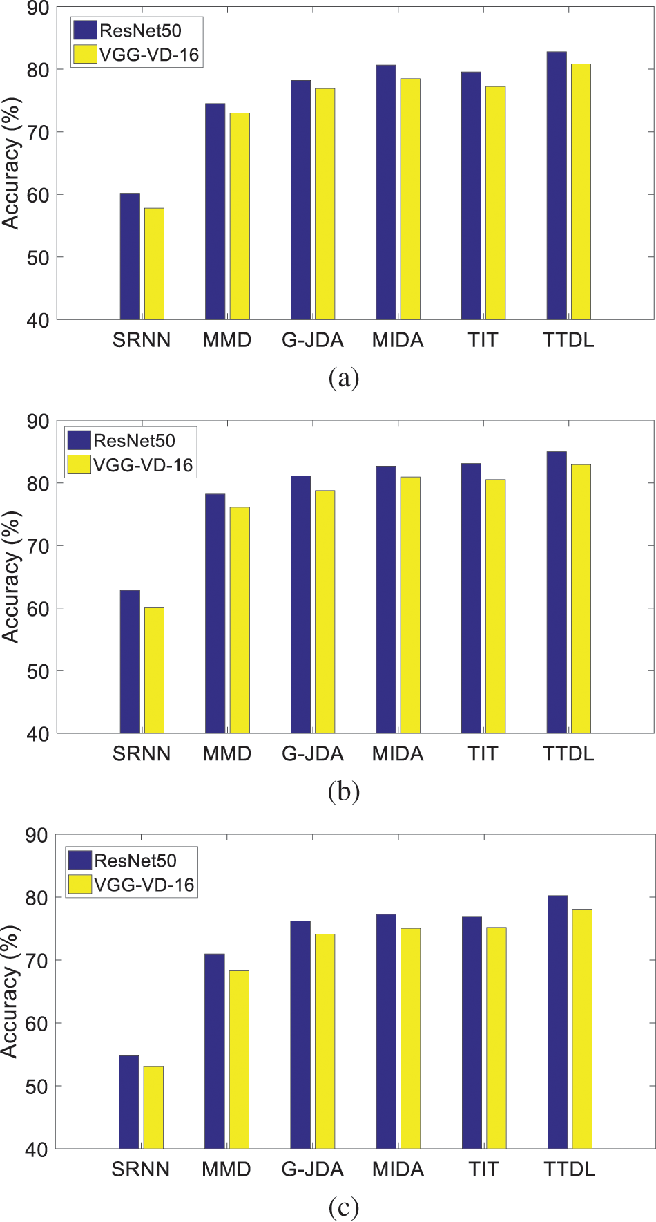
Figure 2: Accuracy comparison of all algorithms in the, (a) U→R task, (b) A→R task, (c) S→R task

4.3 Model Analysis

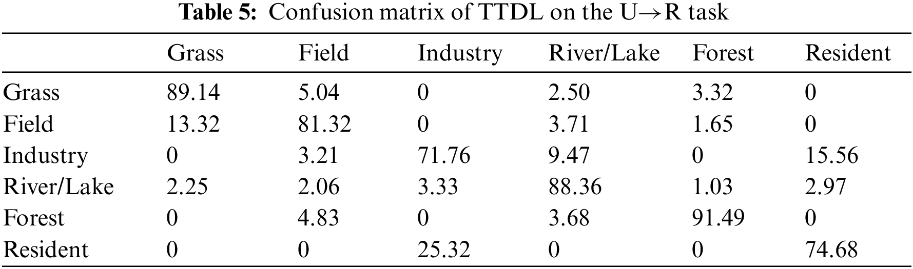
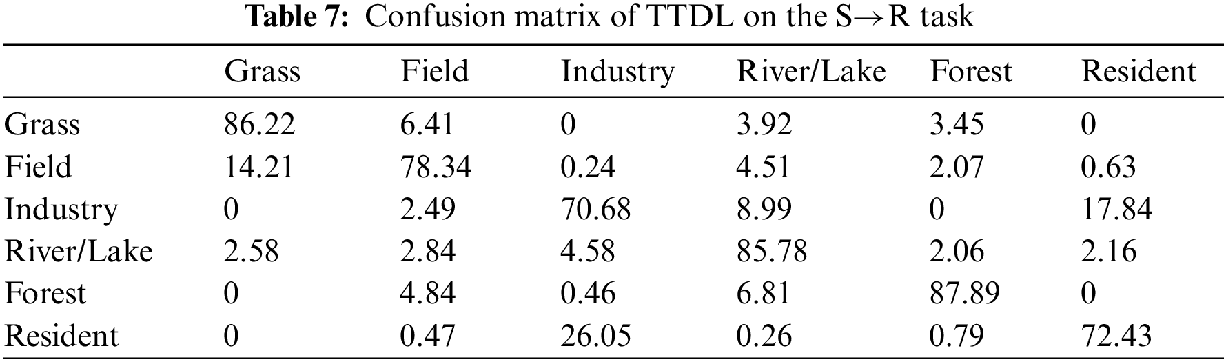
We show the confusion matrix using the ResNet50 feature in Tables 5–7. The value in confusion matrices means the accuracy (%) of TTDL in each class. The testing data of each scene class in the RSSCN7 dataset consists of 380 images. We can see that in the U→R task, TTDL classifies scene classes of Grass, River/Lake, and Forest over 80%, and the accuracy of Industry is low. The reason is mainly that Industry and Resident have the high similarity in the Ucmerced land and RSSCN7 datasets. The performances of TTDL in the A→R and S→R tasks show similar results. The classification performance in Grass, River/Lake, and Forest, are a higher than that of other classes.

4.4 Ablation Experiment

To further analysis three components in TTDL, we show the ablation experiment results using ResNet50 feature in Table 8. TTDL with θ2 = 0 means Φ(P~) is removed. TTDL with θ3 = 0 means Z(D) is removed. TTDL with θ4=δ=0 means Γ(A~,Qt) is removed. The experimental results validate the effectiveness of triplet-induced ordinal locality preserving term, Fisher discriminant term, and graph Laplacian regularization term in TTDL. The triplet-induced ordinal locality preserving term finds a suitable projection subspace to preserve the data structure. The Fisher discriminant term builds a discriminant dictionary to bridge two different domains. The graph Laplacian regularization term learns the discriminant sparse representation. With the joint learning of three terms, the TTDL algorithm has achieved satisfactory results in cross-dataset remote scene image classifications.

5  Conclusion

The ecological environment has become one of the root factors affecting human health. Environmental and health management is a comprehensive and complex work across departments, fields, and disciplines. The rapid development of aerospace, satellite remote sensing, and data communication technology makes the application of remote sensing technology in ecological environmental monitoring more extensive. Reducing the workload of manual annotation and achieving high-precision classification of remote sensing images are difficult problems in ecological environmental monitoring. Benefiting from the previous manual labeling work, there are a large number of labeled datasets in the source domain. Because of the large differences between different datasets, it is difficult to achieve the ideal classification by directly training the classifier with these labeled datasets. To solve this problem, this paper proposes a transductive transfer dictionary learning algorithm TTDL. To obtain the representation of different domain samples, TTDL uses a subspace projection strategy to eliminate the distribution difference. In TTDL, the triplet induced ordinal locality preserving term, Fisher discriminant term, and graph Laplacian regularization term are introduced, so that the dictionary has intra-class compactness and inter-class differences. The TTDL algorithm has achieved satisfactory results in remote sensing image classification across datasets. Our work in the next stage includes integrating statistical information from data into subspace projection to eliminate feature distribution differences. For remote sensing images, the class imbalance often exists; it will lead to a high misclassification rate for classes with fewer samples. How to solve this problem is also our future research work. In addition, the transfer learning algorithm proposed in this paper is only applied to a single feature perspective. How to use multiple feature perspective data to accurately describe the data structure has important research significance and application value.

Funding Statement: This research was funded in part by the Natural Science Foundation of Jiangsu Province under Grant BK 20211333, and by the Science and Technology Project of Changzhou City (CE20215032).

Availability of Data and Materials: Four public datasets RSSCN7, Ucmerced land, SIRI-WHU, and AID are used in this study. The RSSCN7 dataset can be downloaded in https://github.com/palewithout/RSSCN7. The Ucmerced land dataset can be downloaded in http://weegee.vision.ucmerced.edu/datasets/landuse.html. The SIRI-WHU dataset can be downloaded in https://figshare.com/articles/dataset/SIRI_WHU_Dataset/8796980. The AID dataset can be downloaded in https://paperswithcode.com/dataset/aids.

Conflicts of Interest: The authors declare that they have no conflicts of interest to report regarding the present study.

References

1. Zou, Q., Ni, L., Zhang, T., Wang, Q. (2015). Deep learning based feature selection for remote sensing scene classification. IEEE Geoscience and Remote Sensing Letters, 12(11), 2321–2325. [Google Scholar]

2. Yang, Y., Newsam, S. (2010). Bag-of-visual-words and spatial extensions for land-use classification. Proceedings of the 18th SIGSPATIAL International Conference on Advances in Geographic Information Systems, pp. 270–279. San Jose. [Google Scholar]

3. Soltani-Farani, A., Rabiee, H. R., Hosseini, S. A. (2014). Spatial-aware dictionary learning for hyperspectral image classification. IEEE Transactions on Geoscience and Remote Sensing, 53(1), 527–541. [Google Scholar]

4. Vu, T. H., Monga, V. (2017). Fast low-rank shared dictionary learning for image classification. IEEE Transactions on Image Processing, 26(11), 5160–5175. [Google Scholar]

5. Geng, H., Wang, L., Liu, P. (2014). Dictionary learning for large-scale remote sensing image based on particle swarm optimization. 2014 12th International Conference on Signal Processing (ICSP), pp. 784–789. Hangzhou, China. [Google Scholar]

6. Zheng, Z., Zhong, Y., Su, Y., Ma, A. (2022). Domain adaptation via a task-specific classifier framework for remote sensing cross-scene classification. IEEE Transactions on Geoscience and Remote Sensing, 60(2), 1–13. [Google Scholar]

7. Zhang, J., Liu, J., Pan, B., Shi, Z. (2020). Domain adaptation based on correlation subspace dynamic distribution alignment for remote sensing image scene classification. IEEE Transactions on Geoscience and Remote Sensing, 58(11), 7920–7930. [Google Scholar]

8. Zhu, L., Ma, L. (2016). Class centroid alignment based domain adaptation for classification of remote sensing images. Pattern Recognition Letters, 83(11), 124–132. [Google Scholar]

9. Zhou, Z., Wu, Y., Yang, X., Zhou, Y. (2022). Neural style transfer with adaptive auto-correlation alignment loss. IEEE Signal Processing Letters, 29(4), 1027–1031. https://doi.org/10.1109/LSP.2022.3165758 [Google Scholar] [CrossRef]

10. Tuia, D., Marcos, D., Camps-Valls, G. (2016). Multi-temporal and multi-source remote sensing image classification by nonlinear relative normalization. ISPRS Journal of Photogrammetry and Remote Sensing, 120(10), 1–12. [Google Scholar]

11. Wang, D., Wu, J., Yang, J., Jing, B., Zhang, W. et al. (2021). Cross-lingual knowledge transferring by structural correspondence and space transfer. IEEE Transactions on Cybernetics, 52(7), 6555–6566. [Google Scholar]

12. Jiang, Z., Lin, Z., Davis, L. S. (2013). Label consistent K-SVD: Learning a discriminative dictionary for recognition. IEEE Transactions on Pattern Analysis and Machine Intelligence, 35(11), 2651–2664. [Google Scholar] [PubMed]

13. Yang, M., Zhang, L., Feng, X., Zhang, D. (2014). Sparse representation based fisher discrimination dictionary learning for image classification. International Journal of Computer Vision, 109(5), 209–232. [Google Scholar]

14. Qi, L., Huo, J., Fan, X., Shi, Y., Gao, Y. (2018). Unsupervised joint subspace and dictionary learning for enhanced cross-domain person re-identification. IEEE Journal of Selected Topics in Signal Processing, 12(6), 1263–1275. [Google Scholar]

15. Xia, G. S., Hu, J., Hu, F., Shi, B., Bai, X. et al. (2017). AID: A benchmark data set for performance evaluation of aerial scene classification. IEEE Transactions on Geoscience and Remote Sensing, 55(7), 3965–3981. [Google Scholar]

16. Zhao, B., Zhong, Y., Xia, G. S., Zhang, L. (2015). Dirichlet-derived multiple topic scene classification model for high spatial resolution remote sensing imagery. IEEE Transactions on Geoscience and Remote Sensing, 54(4), 2108–2123. [Google Scholar]

17. Zou, J., Li, W., Du, Q. (2015). Sparse representation-based nearest neighbor classifiers for hyperspectral imagery. IEEE Geoscience and Remote Sensing Letters, 12(12), 2418–2422. [Google Scholar]

18. Sejdinovic, D., Sriperumbudur, B., Gretton, A., Fukumizu, K. (2013). Equivalence of distance-based and RKHS-based statistics in hypothesis testing. The Annals of Statistics, 41(5), 2263–2291. [Google Scholar]

19. Hsieh, Y. T., Tao, S. Y., Tsai, Y. H. H., Yeh, Y. R., Wang, Y. C. F. (2016). Recognizing heterogeneous cross-domain data via generalized joint distribution adaptation. 2016 IEEE International Conference on Multimedia and Expo (ICME), pp. 1–6. Seattle. [Google Scholar]

20. Yan, K., Kou, L., Zhang, D. (2017). Learning domain-invariant subspace using domain features and independence maximization. IEEE Transactions on Cybernetics, 48(1), 288–299. [Google Scholar] [PubMed]

21. Li, J., Lu, K., Huang, Z., Zhu, L., Shen, H. T. (2018). Transfer independently together: A generalized framework for domain adaptation. IEEE Transactions on Cybernetics, 49(6), 2144–2155. [Google Scholar] [PubMed]