
 Submit a Paper
 Propose a Special lssue
 Open Access
ARTICLE
Brain Functional Network Generation Using Distribution-Regularized Adversarial Graph Autoencoder with Transformer for Dementia Diagnosis
1
School of Information Engineering, Hubei University of Economics, Wuhan, 430205, China
2
State Key Laboratory of Simulation and Regulation of Water Cycle in River Basin, China Institute of Water Resources
and Hydropower Research, Beijing, 100038, China
3
School of Computing and Mathematic Sciences, University of Leicester, Leicester, LE1 7RH, UK
4
Shenzhen Institutes of Advanced Technology, Chinese Academy of Sciences, Shenzhen, 518055, China
5
Faculty of Science and Technology, University of Macau, Macau, 999078, China
6
School of Geophysics, Chengdu University of Technology, Chengdu, 610059, China
7
Laboratory of Artificial Intelligence and 3D Technologies for Cardiovascular Diseases, Guangdong Provincial Key Laboratory
of South China Structural Heart Disease, Guangdong Provincial People’s Hospital (Guangdong Academy of Medical Sciences),
Southern Medical University, Guangzhou, 519041, China
8
Medical Research Institute, Guangdong Provincial People’s Hospital (Guangdong Academy of Medical Sciences),
Southern Medical University, Guangzhou, 519041, China
* Corresponding Authors: Yudong Zhang. Email: ; Jin Hong. Email:
Computer Modeling in Engineering & Sciences 2023, 137(3), 2129-2147. https://doi.org/10.32604/cmes.2023.028732
Received 04 January 2023; Accepted 20 March 2023; Issue published 03 August 2023
 View Full Text
 Download PDF
Abstract
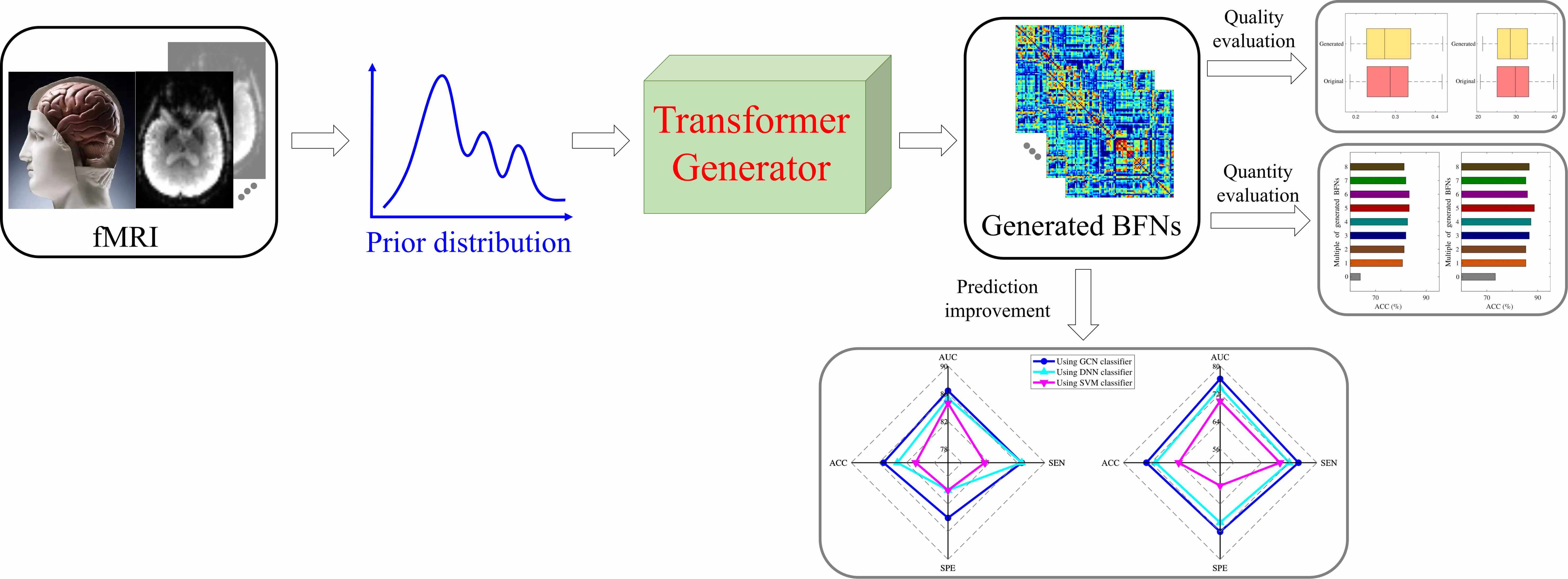
The topological connectivity information derived from the brain functional network can bring new insights for diagnosing and analyzing dementia disorders. The brain functional network is suitable to bridge the correlation between abnormal connectivities and dementia disorders. However, it is challenging to access considerable amounts of brain functional network data, which hinders the widespread application of data-driven models in dementia diagnosis. In this study, a novel distribution-regularized adversarial graph auto-Encoder (DAGAE) with transformer is proposed to generate new fake brain functional networks to augment the brain functional network dataset, improving the dementia diagnosis accuracy of data-driven models. Specifically, the label distribution is estimated to regularize the latent space learned by the graph encoder, which can make the learning process stable and the learned representation robust. Also, the transformer generator is devised to map the node representations into node-to-node connections by exploring the long-term dependence of highly-correlated distant brain regions. The typical topological properties and discriminative features can be preserved entirely. Furthermore, the generated brain functional networks improve the prediction performance using different classifiers, which can be applied to analyze other cognitive diseases. Attempts on the Alzheimer’s Disease Neuroimaging Initiative (ADNI) dataset demonstrate that the proposed model can generate good brain functional networks. The classification results show adding generated data can achieve the best accuracy value of 85.33%, sensitivity value of 84.00%, specificity value of 86.67%. The proposed model also achieves superior performance compared with other related augmented models. Overall, the proposed model effectively improves cognitive disease diagnosis by generating diverse brain functional networks.Graphic Abstract
Keywords
The brain is an information-processing system with many complicated and precise computations when dealing with various daily activities [1]. Daily physiological activities are always associated with the interaction between multiple neurons, neuronal clusters, or multiple brain regions. This interaction is called brain functional network (BFN), which describes the relationship between temporal blood-oxygen-level-dependent (BOLD) signals from distant brain areas [2]. Dementia (i.e., Alzheimer’s Disease, AD) is a typical kind of neuropathic disorder where patients usually show abnormal functional connections between brain regions [3]. It can result in a series of cognitive symptoms: memory impairment, poor language expression, and changes in vision [4,5]. Functional magnetic resonance imaging (fMRI) can easily capture these abnormal features using the non-intrusive scanning technology [6]. The BFN can bring a new way for the diagnosis and analysis of neurodegenerative disorders [7]. Therefore, analysis of BFNs is important to mine complex brain connectivity features and help detect dementia-related biomarkers. It is further important to understand the pathogenic mechanism and the drug discovery for neurodegenerative disorders [8].
The BFN is usually constructed through a software toolbox by splitting the human brain into predefined Region-of-Interests (ROIs) [9]. The element in the BFN matrix indicates the functional correlation between two ROIs. Many approaches based on machine learning were utilized to diagnose neurological disease in an end-to-end scheme [10–16]. For example, Meier et al. [17] applied the support vector machine (SVM) classifier to distinguish older adults from younger adults using functional connectivity data. To boost the Mild Cognitive Impairment (MCI) prediction performance, Yu et al. [18] designed a sparse graph representation learning method with a weighting scheme to generate sparse BFNs. Bi et al. [19] combined convolutional learning and recurrent learning to extract regional connectivity and adjacent positional features, which proves its learning ability in AD diagnosis. More advanced techniques are proposed to explore the complex connectivity-based features [20–22]. Ji et al. [23] devised novel convolutional kernels to capture hierarchical topological characteristics by element-wise weighting brain networks and achieved more accurate classification performance. The work in [24] applied the graph convolutional network (GCN) method to improve the classification accuracy by jointly using the functional time series and connectivity-based matrices. Nevertheless, the limited medical data makes data-driven models challenging to achieve good prediction results.
The straightforward way to improve classification performance is to synthesize more similar medical data and feed it to data-driven models [25,26]. Numerous data-augmented methods have been developed to solve the small data problem in the field of brain imaging analysis. For example, Hong et al. [27] augmented the routine brain magnetic resonance (MR) imaging with scaling, rotation, translation, and gamma correction and achieved accurate results predicting children’s brain age through a deep learning model. Hu et al. [28] synthesized the positron emission tomography (PET) from MR using generative models, which can handle the problem of incomplete modalities and is promising for multimodal fusion. However, the above methods cannot be applied to BFN augmentation, because it only considers the local features between adjacent pixels and ignores the topological information between distant pixels. Many efforts have been tried to generate new graph data in the graph domain. Meszlényi et al. [29] created some simulated connectivity-based datasets by applying noise weights (NW) to improve the classification performance. The study of [30] solved the problem of small-size data by employing the synthetic minority over-sampling technique (SMOTE) algorithm and achieved a good classification accuracy of non-tumorous facial pigmentation disorders. However, these methods do not directly generate new graph data but interpolate existing brain networks to augment the data, which brings some noise and may have some side effects on the model’s classification performance.
The generative adversarial networks (GANs) [31] is a two-player game that can produce quite good results by mutual game learning [32]. It has gained broad applications in analyzing medical imaging because of its strong ability in distribution fitting [33]. These applications cover the image-related fields, including cross-modal synthesis [34], point cloud generation [35], image super-resolution [36], disease classification [37–39], regression task [40,41], and organ segmentation [42]. Besides, the prior distribution can guide the model’s optimization and thus stabilize the representation learning in the GAN’s training [43]. Reference [44] introduced a Gaussian distribution to constrain the graph embedding in adversarial learning and achieved good performance in graph analytics. The GAN-based model has been applied in the BFN augmentation. For example, Tan et al. [45] utilized the Gaussian noise to synthesize BFNs by applying a semi-positive definite manifold constraint. Also, the transformer network [46] can greatly improve image classification performance by combining adversarial strategy, which can model a strong relationship between distant ROIs.
Motivated by these observations, in this study, a novel distribution-regularized adversarial graph autoencoder (DAGAE) model is proposed to generate BFNs for dementia diagnosis. The main works of this paper are as follows: (1) The label distribution is estimated to regularize the latent space learned by the graph encoder, which can make the learning process stable and deduce a robust representation. (2) The transformer-based network in the generator is introduced to map the node representations into node-to-node connections by exploring the global connectivity information between distant ROIs. It preserves the main topological properties and more discriminative features. (3) The generated BFNs enhance disease prediction using different classifiers, which can be applied to analyze other related brain diseases.
The purpose of the Alzheimer’s Disease Neuroimaging Initiative (ADNI) project1 1 http://adni.loni.usc.edu/ is to detect the early stage of Alzheimer’s disease from clinical, imaging, gene, biomarker, and other aspects. In this study, we mainly focus on the Late Mild Cognitive Impairment (LMCI) stage scanned with functional Magnetic Resonance Imaging (fMRI). To eliminate the influence of category imbalance on model classification performance, we selected the same number of NC subjects as LMCI for the experiment. About 150 subjects with fMRI were selected to test our model’s effectiveness, including 75 Normal Controls (NC) and 75 LMCI. The fMRI data were scanned with the filed strength of
The commonly used GRETNA [47] software is adopted to preprocess the fMRI to construct graph data. The detailed procedures include format conversion, first ten volumes removal, slice timing, head motion realign, normalizing, spatially smooth, detrend, and temporally filtering (usually
2.2 Distribution-Regularized Adversarial Graph Autoencoder
The BFN is generated by the designed DAGAE model, which is depicted in Fig. 1. It accepts the graph data (including brain functional feature F and BFN

Figure 1: The architecture of the proposed DAGAE model. It accepts brain functional feature F and BFN
2.2.1 Label Distribution Estimation
To improve the performance of node representation in latent space, the label probability distribution estimated by Kernel Density Estimation (KDE) is introduced in the node representation learning. Instead of the traditional normal distribution, it can reflect the accurate distribution of node features and ensure robust representations in the model training. In the feature space, the node feature
where,
2.2.2 Adversarial Graph Encoder
The graph encoder accepts both F and
The node representation H is treated as a fake sample to send to the discriminator
The graph encoder aims to enforce the latent node representation H to be consistent with the estimated label distribution

Figure 2: Illustration of the discriminator and classifier structure. The input of the discriminator is a matrix computed from either latent node representation H or label distribution
In addition, to make the node representation discriminative, the cross-entropy loss is introduced to further regularize the learned node representation. The binary classifier
here, the
The transformer generator
The reconstruction loss is adopted to preserve the original graph structure while making the autoencoder training stable. We choose the L1 norm to measure the distance between the original
Moreover, to make the generator learning more stable, we put the reconstructed brain network
2.3 Classification Training and Evaluation Metrics
In summary, the optimization strategy of the proposed DAGAE updates the weights of the graph encoder, discriminator, classifier, and transformer generator. The hybrid loss is defined by:
As illustrated in Fig. 3, we send the training set to the DAGAE model for training and augment the BFN with the transformer generator. The detailed training of the DAGAE model is shown in Algorithm 1. Inspired by the method [49,50], the latent feature learning can be stable when the optimization converges. For each label (i.e., NC and LMCI), we sample matrics from the distribution

Figure 3: The entire workflow of this work. In the training stage, the transformer generator is first extracted from the trained DAGAE and then maps the distribution-sampled representation into generated BFNs (
In the classification stage, we build a sample graph classifier modified from [24], including two GCN layers with 32 and 16 hidden neurons, one graph pooling, and one MLP layer with two neurons. The original training set is first used to train the graph classifier. Then the generated BFNs are mixed in the training set to finetune the classifier for enhancing classification performance. At last, the trained classifier predicts disease labels of the testing set for performance evaluation. There are four commonly used metrics for the prediction assessment: Accuracy (ACC), Specificity (SPE), Sensitivity (SEN), and the Area Under the receiver operating characteristic Curve (AUC). They are defined as:
where, TN means that NC is correctly predicted, TL means that LMCI is correctly predicted. FN means that NC is incorrectly predicted, FL means that LMCI is incorrectly predicted.

We adopt the 5-fold cross-validation strategy in the experiment to conduct the training and testing. The preprocessed data is evenly separated into five folds, meaning each fold contains 15 NCs and 15 LMCIs. We first selected one-fold data and sent the rest of the four folds data (60 NCs and 60 LMCIs) into the DAGAE model for training. Next, the trained generator is used to generate
The DAGAE is trained on Ubuntu18.04 using the TensorFlow framework for BFN synthesis. The graphical device is one GPU with NVIDIA Quadro P4000 8.0 GB. We set the model’s parameters with the values as follows:
In the experiment, it is essential to constrain the latent node representation to follow the label distribution. This constraint can diminish the model overfitting and stabilize the representation learning. Fig. 4 shows the adversarial loss over epochs in the training process. In the beginning, the encoder loss falls, and the discriminator rises. After 250 epochs, both keep around 0.5 steadily, which means the adversarial training converges. After the training, the transformer generator generates new BFNs by accepting node representation matrices sampled from the label distribution

Figure 4: The loss curve of the adversarial training. It is utilized to constrain the latent node representations in the label distribution

Figure 5: Visualization of the original and generated BFNs. The left column shows the original BFNs at NC and LMCI stages, and the right column shows the generated BFNs at NC and LMCI stages
We analyze the classification performance with different classifiers to investigate the proposed model’s effectiveness. As shown in Table 1, the generated BFNs can gain better classification performance over original BFNs. Among the three augmented methods, our model achieved superior results in three classifiers with more than 10 percent of ACC value compared to results using original BFNs. Also, our model increases the ACC value by 1.3%, 2.0%, and 3.3% compared with the competing ARAE method for GCN, DNN, and SVM classifiers, respectively. This evidence proves that the proposed model can generate more effective BFNs for classification improvement. To detail the effectiveness of the GCN-based classifier, Figs. 6a and 6b show that the prediction results using a GCN-based classifier achieves the best performance than other traditional classifiers. Note that both original and generated BFNs using different methods are sent to the same classifier for classification performance evaluation. Fig. 7 also shows better performance of the GCN-based classifier. Our model shows superior prediction performance in terms of ACC, SEN, SPE, and AUC by achieving 85.33%, 84.0%, 86.67%, and 86.42%. It probably indicates that the GCN-based classifier can benefit the topological properties buried in the BFNs and enhance the classification of BFNs.


Figure 6: The prediction performance comparison using three classifiers by inputting BFNs from (a) our model, (b) original

Figure 7: The comparison of ROC curves using three classifiers. The gray dotted line represents the random classifier
3.3 Evaluation of the Generated BFNs
In this section, we evaluate the coherence between original and generated BFNs. We generated the same size as the original data in each one-fold training. We employed the t-distributed Stochastic Neighbour Embedding (t-SNE) tool [54] to analyze the graphical characteristics. Fig. 8 shows the projection of the embedding representation of original and generated BFNs from high-dimensional space to two-dimensional space. The generated data is consistent with the original data distribution, which ensures the similarity between the generated and original FBNs. In addition, six common metrics are utilized to quantitatively measure the effectiveness of the generated data. These six metrics can provide a relatively reliable measure of generated BFN’s quality, including clustering coefficient, node strength, betweenness centrality, modularity, local efficiency, and global efficiency. As shown in Fig. 9, the boxplot distribution of each metric is compared between the generated and original BFNs. The generated data can mostly cover the range of graph metrics from the original data. Therefore, the generated BFNs by our model contains non-Euclidean characteristics and preserve the overall nature of brain connectivity, which is suitable to augment the BFNs for dementia diagnosis.
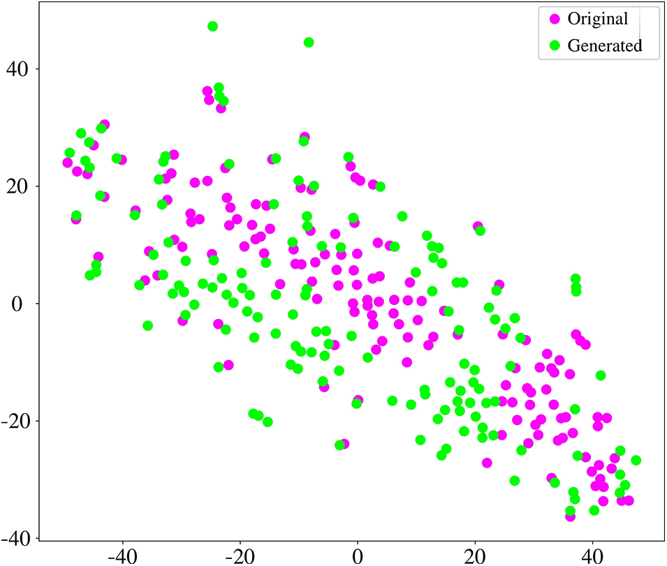
Figure 8: The comparison of embedded t-SNE representation between the original and generated BFNs

Figure 9: Statistical analysis of the original and generated BFN. (A) Cluster coefficient, (B) Node strength, (C) Betweenness centrality, (D) Modularity, (E) Global efficiency, and (F) Local efficiency
The proposed DAGAE model can generate new BFNs for improving classification performance. Each module in the model contributes to the generation quality of BFNs. To analyze the influence of different modules, we remove the encoder, discriminator, and classifier from the DAGAE model and evaluate the final classification performance. Fig. 10 demonstrates that the encoder significantly impacts the whole model. It drops by 16% in terms of ACC by removing the encoder module. The discriminator ensures the latent node representation in a prior distribution, which also influences the quality of the generated BFNs. This suggests the usefulness of prior label distribution can regularize the latent representation with a stable learning strategy and enhance the BFN classification. Furthermore, we study the dimension

Figure 10: Influence of different modules on the classification performance. (a) The proposed DAGAE, (b) DAGAE without encoder, (c) DAGAE without discriminator, and (d) DAGAE without the classifier

Figure 11: Impact of the dimension

Data-driven models achieve better performance by using large amounts of data. To investigate how much generated data influences the prediction performance, we generate

Figure 12: Classification accuracy analysis using different amounts of generated data by our model using (a) SVM and (b) GCN classifier, respectively
Although the proposed DAGAE is promising in augmenting the BFN data for disease prediction, there are still two limitations that have not been considered. (1) The label distribution is estimated using the limited training data, which can not add other prior knowledge. We will introduce disease-related anatomical brain knowledge into the model for performance evaluation. (2) The data in this work are deliberately picked out to maintain category balance. The real condition in the category distribution is always imbalanced. In the following study, we will try to apply the proposed DAGAE in category-imbalanced datasets for other brain disorder diagnosis.
This study proposes a novel DAGAE model to augment new BFNs for dementia diagnosis. The BFN augmentation is different from traditional image synthesis, where the latter only extracts local patterns and ignores the topological information buried in the brain network. Our model is novel in two aspects. One is that the estimated label distribution can regularize the latent space and make the learning process stable. Another one is that the transformer generator is devised to map the node representations into node-to-node connections by exploring the long-term dependence of highly-correlated distant brain regions, which preserves the main topological properties and more discriminative features. Testing on the Alzheimer’s Disease Neuroimaging Initiative (ADNI) public dataset, the proposed DAGAE can generate similar and high-quality BFNs. The classification results show that adding generated data can achieve higher accuracy values of 85.33%, 83.33%, and 80.67% than the original method using GCN, DNN, and SVM classifiers, respectively. The proposed model also performs better than related augmented models, providing new insight for improving cognitive disease diagnosis accuracy.
Funding Statement: This paper is partially supported by the British Heart Foundation Accelerator Award, UK (AA∖18∖3∖34220); Royal Society International Exchanges Cost Share Award, UK (RP202G0230); Hope Foundation for Cancer Research, UK (RM60G0680); Medical Research Council Confidence in Concept Award, UK (MC_PC_17171); Sino-UK Industrial Fund, UK (RP202G0289); Global Challenges Research Fund (GCRF), UK (P202PF11); LIAS Pioneering Partnerships Award, UK (P202ED10); Data Science Enhancement Fund, UK (P202RE237); Fight for Sight, UK (24NN201); Sino-UK Education Fund, UK (OP202006); Biotechnology and Biological Sciences Research Council, UK (RM32G0178B8); LIAS Seed Corn, UK (P202RE969).
Conflicts of Interest: The authors declare that they have no conflicts of interest to report regarding the present study.
References
1. Samarasinghe, R. A., Miranda, O. A., Buth, J. E., Mitchell, S., Ferando, I. et al. (2021). Identification of neural oscillations and epileptiform changes in human brain organoids. Nature Neuroscience, 24(10), 1488–1500. [Google Scholar] [PubMed]
2. Suárez, L. E., Markello, R. D., Betzel, R. F., Misic, B. (2020). Linking structure and function in macroscale brain networks. Trends in Cognitive Sciences, 24(4), 302–315. [Google Scholar]
3. Schumacher, J., Peraza, L. R., Firbank, M., Thomas, A. J., Kaiser, M. et al. (2019). Dynamic functional connectivity changes in dementia with lewy bodies and alzheimer’s disease. NeuroImage: Clinical, 22(37), 101812. [Google Scholar] [PubMed]
4. Borelli, C. M., Grennan, D., Muth, C. C. (2020). Causes of memory loss in elderly persons. JAMA, 323(5), 486–486. [Google Scholar] [PubMed]
5. Berron, D., Vogel, J. W., Insel, P. S., Pereira, J. B., Xie, L. et al. (2021). Early stages of tau pathology and its associations with functional connectivity, atrophy and memory. Brain, 144(9), 2771–2783. [Google Scholar] [PubMed]
6. Fu, Z., Caprihan, A., Chen, J., Du, Y., Adair, J. C. et al. (2019). Altered static and dynamic functional network connectivity in alzheimer’s disease and subcortical ischemic vascular disease: Shared and specific brain connectivity abnormalities. Human Brain Mapping, 40(11), 3203–3221. [Google Scholar] [PubMed]
7. Chen, M., Li, H., Wang, J., Dillman, J. R., Parikh, N. A. et al. (2019). A multichannel deep neural network model analyzing multiscale functional brain connectome data for attention deficit hyperactivity disorder detection. Radiology: Artificial Intelligence, 2(1), e190012. [Google Scholar] [PubMed]
8. Ma, W. Y., Yao, Q., Hu, G. J., Ge, H. L., Xue, C. et al. (2022). Reorganization of rich clubs in functional brain networks of dementia with lewy bodies and alzheimer’s disease. NeuroImage: Clinical, 33(12), 102930. [Google Scholar] [PubMed]
9. Zuo, Q., Lei, B., Shen, Y., Liu, Y., Feng, Z. et al. (2021). Multimodal representations learning and adversarial hypergraph fusion for early alzheimer’s disease prediction. Chinese Conference on Pattern Recognition and Computer Vision (PRCV), Beijing, China, Springer. [Google Scholar]
10. Teipel, S. J., Wohlert, A., Metzger, C., Grimmer, T., Sorg, C. et al. (2017). Multicenter stability of resting state fMRI in the detection of alzheimer’s disease and amnestic MCI. NeuroImage: Clinical, 14(Suppl. 3), 183–194. [Google Scholar] [PubMed]
11. Ahmed, M. R., Zhang, Y., Feng, Z., Lo, B., Inan, O. T. et al. (2018). Neuroimaging and machine learning for dementia diagnosis: Recent advancements and future prospects. IEEE Reviews in Biomedical Engineering, 12, 19–33. [Google Scholar] [PubMed]
12. Wang, S., Wang, H., Shen, Y., Wang, X. (2018). Automatic recognition of mild cognitive impairment and alzheimers disease using ensemble based 3D densely connected convolutional networks. 2018 17th IEEE International Conference on Machine Learning and Applications (ICMLA), Orlando, FL, USA, IEEE. [Google Scholar]
13. Hong, J., Wang, S. H., Cheng, H., Liu, J. (2020). Classification of cerebral microbleeds based on fully-optimized convolutional neural network. Multimedia Tools and Applications, 79(21), 15151–15169. [Google Scholar]
14. Yu, W., Lei, B., Wang, S., Liu, Y., Feng, Z. et al. (2022). Morphological feature visualization of alzheimer’s disease via multidirectional perception GAN. IEEE Transactions on Neural Networks and Learning Systems, 1–15. USA, IEEE. https://doi.org/10.1109/TNNLS.2021.3118369 [Google Scholar] [PubMed] [CrossRef]
15. Zong, Y., Jing, C., Zuo, Q. (2022). Multiscale autoencoder with structural-functional attention network for alzheimer’s disease prediction. Chinese Conference on Pattern Recognition and Computer Vision (PRCV), Shenzhen, China, Springer. [Google Scholar]
16. Sheykhivand, S., Rezaii, T. Y., Mousavi, Z., Delpak, A., Farzamnia, A. (2020). Automatic identification of epileptic seizures from EEG signals using sparse representation-based classification. IEEE Access, 8, 138834–138845. [Google Scholar]
17. Meier, T. B., Desphande, A. S., Vergun, S., Nair, V. A., Song, J. et al. (2012). Support vector machine classification and characterization of age-related reorganization of functional brain networks. NeuroImage, 60(1), 601–613. [Google Scholar] [PubMed]
18. Yu, R., Qiao, L., Chen, M., Lee, S. W., Fei, X. et al. (2019). Weighted graph regularized sparse brain network construction for MCI identification. Pattern Recognition, 90, 220–231. [Google Scholar] [PubMed]
19. Bi, X., Zhao, X., Huang, H., Chen, D., Ma, Y. (2020). Functional brain network classification for alzheimer’s disease detection with deep features and extreme learning machine. Cognitive Computation, 12(3), 513–527. [Google Scholar]
20. Kawahara, J., Brown, C. J., Miller, S. P., Booth, B. G., Chau, V. et al. (2017). BrainNetCNN: Convolutional neural networks for brain networks; towards predicting neurodevelopment. NeuroImage, 146(4), 1038–1049. [Google Scholar] [PubMed]
21. Yu, S., Wang, S., Xiao, X., Cao, J., Yue, G. et al. (2020). Multi-scale enhanced graph convolutional network for early mild cognitive impairment detection. International Conference on Medical Image Computing and Computer-Assisted Intervention, Lima, Peru, Springer. [Google Scholar]
22. Xiao, L., Wang, J., Kassani, P. H., Zhang, Y., Bai, Y. et al. (2019). Multi-hypergraph learning-based brain functional connectivity analysis in fMRI data. IEEE Transactions on Medical Imaging, 39(5), 1746–1758. [Google Scholar] [PubMed]
23. Ji, J., Xing, X., Yao, Y., Li, J., Zhang, X. (2021). Convolutional kernels with an element-wise weighting mechanism for identifying abnormal brain connectivity patterns. Pattern Recognition, 109(16), 107570. [Google Scholar]
24. Zuo, Q., Lu, L., Wang, L., Zuo, J., Ouyang, T. (2022). Constructing brain functional network by adversarial temporal-spatial aligned transformer for early AD analysis. Frontiers in Neuroscience, 16, 108815. [Google Scholar]
25. Ren, Z., Zhang, Y., Wang, S. (2022). Lcdae: Data augmented ensemble framework for lung cancer classification. Technology in Cancer Research & Treatment, 21(5), 15330338221124372. [Google Scholar]
26. Ramaraj, K., Govindaraj, V., Zhang, Y. D., Murugan, P. R., Thiyagarajan, A. (2021). Brain anomaly prediction with the intervention of fuzzy based clustering and optimization techniques for augmenting clinical diagnosis. 2021 3rd International Conference on Advances in Computing, Communication Control and Networking (ICAC3N), Greater Noida, India, IEEE. [Google Scholar]
27. Hong, J., Feng, Z., Wang, S. H., Peet, A., Zhang, Y. D. et al. (2020). Brain age prediction of children using routine brain MR images via deep learning. Frontiers in Neurology, 11, 584682. [Google Scholar] [PubMed]
28. Hu, S., Lei, B., Wang, S., Wang, Y., Feng, Z. et al. (2021). Bidirectional mapping generative adversarial networks for brain MR to pet synthesis. IEEE Transactions on Medical Imaging, 41(1), 145–157. [Google Scholar] [PubMed]
29. Meszlényi, R. J., Buza, K., Vidnyánszky, Z. (2017). Resting state fMRI functional connectivity-based classification using a convolutional neural network architecture. Frontiers in Neuroinformatics, 11, 61. [Google Scholar]
30. Gao, R., Peng, J., Nguyen, L., Liang, Y., Thng, S. et al. (2019). Classification of non-tumorous facial pigmentation disorders using deep learning and smote. 2019 IEEE International Symposium on Circuits and Systems (ISCAS), Sapporo, Japan, IEEE. [Google Scholar]
31. Goodfellow, I., Pouget-Abadie, J., Mirza, M., Xu, B., Warde-Farley, D. et al. (2020). Generative adversarial networks. Communications of the ACM, 63(11), 139–144. [Google Scholar]
32. Hong, J., Yu, S. C. H., Chen, W. (2022). Unsupervised domain adaptation for cross-modality liver segmentation via joint adversarial learning and self-learning. Applied Soft Computing, 121, 108729. [Google Scholar]
33. Hu, S., Shen, Y., Wang, S., Lei, B. (2020). Brain MR to pet synthesis via bidirectional generative adversarial network. International Conference on Medical Image Computing and Computer-Assisted Intervention, Cham, Springer. [Google Scholar]
34. Hu, S., Yuan, J., Wang, S. (2019). Cross-modality synthesis from MRI to pet using adversarial U-Net with different normalization. 2019 International Conference on Medical Imaging Physics and Engineering (ICMIPE), Shenzhen, China, IEEE. [Google Scholar]
35. Hu, B., Lei, B., Shen, Y., Liu, Y., Wang, S. (2021). A point cloud generative model via tree-structured graph convolutions for 3D brain shape reconstruction. Chinese Conference on Pattern Recognition and Computer Vision (PRCV), Beijing, China, Springer. [Google Scholar]
36. You, S., Lei, B., Wang, S., Chui, C. K., Cheung, A. C. et al. (2022). Fine perceptive gans for brain MR image super-resolution in wavelet domain. IEEE Transactions on Neural Networks and Learning Systems, pp. 1–13. USA, IEEE. https://doi.org/10.1109/TNNLS.2022.3153088 [Google Scholar] [CrossRef]
37. Wang, S., Wang, X., Hu, Y., Shen, Y., Yang, Z. et al. (2020). Diabetic retinopathy diagnosis using multichannel generative adversarial network with semisupervision. IEEE Transactions on Automation Science and Engineering, 18(2), 574–585. [Google Scholar]
38. Yu, W., Lei, B., Ng, M. K., Cheung, A. C., Shen, Y. et al. (2021). Tensorizing gan with high-order pooling for alzheimer’s disease assessment. IEEE Transactions on Neural Networks and Learning Systems, 33(9),4945–4959. [Google Scholar]
39. Sheykhivand, S., Mousavi, Z., Mojtahedi, S., Rezaii, T. Y., Farzamnia, A. et al. (2021). Developing an efficient deep neural network for automatic detection of COVID-19 using chest x-ray images. Alexandria Engineering Journal, 60(3), 2885–2903. [Google Scholar]
40. Lei, B., Liang, E., Yang, M., Yang, P., Zhou, F. et al. (2022). Predicting clinical scores for alzheimer’s disease based on joint and deep learning. Expert Systems with Applications, 187(3), 115966. [Google Scholar]
41. Hu, D., Zhang, H., Wu, Z., Wang, F., Wang, L. et al. (2020). Disentangled-multimodal adversarial autoencoder: Application to infant age prediction with incomplete multimodal neuroimages. IEEE Transactions on Medical Imaging, 39(12), 4137–4149. [Google Scholar] [PubMed]
42. Hong, J., Zhang, Y. D., Chen, W. (2022). Source-free unsupervised domain adaptation for cross-modality abdominal multi-organ segmentation. Knowledge-Based Systems, 250, 109155. [Google Scholar]
43. Zuo, Q., Lei, B., Wang, S., Liu, Y., Wang, B. et al. (2021). A prior guided adversarial representation learning and hypergraph perceptual network for predicting abnormal connections of alzheimer’s disease. arXiv preprint arXiv:2110.09302. [Google Scholar]
44. Pan, S., Hu, R., Long, G., Jiang, J., Yao, L. et al. (2018). Adversarially regularized graph autoencoder for graph embedding. arXiv preprint arXiv:1802.04407. [Google Scholar]
45. Tan, Y. F., Ting, C. M., Noman, F., Phan, R. C. W., Ombao, H. (2022). Graph-regularized manifold-aware conditional wasserstein gan for brain functional connectivity generation. arXiv preprint arXiv:2212.05316. [Google Scholar]
46. Jiang, Y., Chang, S., Wang, Z. (2021). Transgan: Two pure transformers can make one strong gan, and that can scale up. Advances in Neural Information Processing Systems, 34, 14745–14758. [Google Scholar]
47. Wang, J., Wang, X., Xia, M., Liao, X., Evans, A. et al. (2015). GRETNA: A graph theoretical network analysis toolbox for imaging connectomics. Frontiers in Human Neuroscience, 9, 386. [Google Scholar] [PubMed]
48. Tzourio-Mazoyer, N., Landeau, B., Papathanassiou, D., Crivello, F., Etard, O. et al. (2002). Automated anatomical labeling of activations in SPM using a macroscopic anatomical parcellation of the MNI MRI single-subject brain. NeuroImage, 15(1), 273–289. [Google Scholar] [PubMed]
49. Mahajan, S., Pandit, A. K. (2021). Hybrid method to supervise feature selection using signal processing and complex algebra techniques. Multimedia Tools and Applications, 82(4), 1–22. [Google Scholar]
50. Mahajan, S., Abualigah, L., Pandit, A. K., Altalhi, M. (2022). Hybrid aquila optimizer with arithmetic optimization algorithm for global optimization tasks. Soft Computing, 26(10), 4863–4881. [Google Scholar]
51. Hearst, M. A., Dumais, S. T., Osuna, E., Platt, J., Scholkopf, B. (1998). Support vector machines. IEEE Intelligent Systems and their Applications, 13(4), 18–28. [Google Scholar]
52. Kong, Y., Gao, J., Xu, Y., Pan, Y., Wang, J. et al. (2019). Classification of autism spectrum disorder by combining brain connectivity and deep neural network classifier. Neurocomputing, 324, 63–68. [Google Scholar]
53. Kipf, T. N., Welling, M. (2016). Semi-supervised classification with graph convolutional networks. arXiv preprint arXiv:1609.02907. [Google Scholar]
54. van der Maaten, L., Hinton, G. (2008). Visualizing data using t-SNE. Journal of Machine Learning Research, 9(11), 2579–2605. [Google Scholar]
Cite This Article
 Copyright © 2023 The Author(s). Published by Tech Science Press.
This work is licensed under a Creative Commons Attribution 4.0 International License , which permits unrestricted use, distribution, and reproduction in any medium, provided the original work is properly cited.
 Downloads
 Citation Tools