Sonar Image Target Detection for Underwater Communication System Based on Deep Neural Network

1  Introduction

Ocean resources belong to sustainable, green and clean renewable energy. The exploration and development of ocean resources, the research of marine environment monitoring network and underwater sensor network have become important research fields [1]. The sonar detection device is an important tool for the exploration of ocean resources and underwater environment. By building a distributed sonar cooperative networking control system underwater, the functions of intelligent collection, processing and transmission of marine environmental information can be realized, which will greatly help the intelligent integration and reconstruction of marine environmental elements and the subsequent development and utilization of new renewable energy [2–4].

Compared with optical sensors that are limited by imaging distance [5], acoustic instruments, such as side scan sonar and forward-looking sonar images, are widely used because of their advantages in imaging conditions, distance and range [6]. However, due to the influence of equipment and reverberation, sonar images are characterized by low signal-to-noise ratio and severe noise interference [7]. In addition, when the target object is far from the sonar, the size of the target is small relative to the whole sonar image, which is easily mistaken for noise. These problems bring many difficulties to target detection. Therefore, reducing noise interference and realizing fast, accurate and low false alarm rate automatic detection of small underwater targets have become an urgent problem to be solved.

At present, the sonar target detection task is mainly completed by the method of manual recognition, but this method cannot complete the real-time detection task and ensure the accuracy of detection [8–11]. With the development of computer vision, many target detection models have been proposed. These models have been widely used in various target detection tasks [12–14], and they can complete the corresponding detection tasks accurately and in real time. In recent years, due to the strong feature extraction capability, convolutional neural network (CNN) has been widely used as a feature extractor for various task scenes such as image classification [15], target detection [16], target tracking [17] and semantic segmentation [18]. Generally speaking, target detection models based on CNN can be divided into two categories of anchor based method and anchor free method. The anchor based method is divided into one stage and two stages: the classical two-stage detection model RCNN series [19–21] and the classical one-stage detection model YOLO series [22–24], SSD [25], and RefineDet [26]. Generally, the two-stage model’s detection speed is slower than that of the first stage, but the accuracy of the two-stage detection model is higher than that of the first stage. However, the method based on anchor increases the computational complexity, due to having too many anchors, and brings a large number of parameters that also affect the detection performance of the model. Based on this problem, researchers have proposed target detection models based on anchor free method, such as Cornernet [27], Centernet [28] and FCOS [29]. The anchor free method abandons the idea of anchor and realizes detection by determining the key points (center point, diagonal point, etc.) of the target object, which greatly reduces the number of network parameters and realizes the best trade-off between accuracy and speed. Since there are two predictions for anchor frames in the model that we created, it will go through two NMS if we use the anchor-frame-based model, which significantly increases the computational work of the model. As a result, we use the anchor-free CenterNet model to improve the model and perform anchor frame regression using the centroid regression approach. The model’s training and prediction times are also significantly reduced by using the NMS-free prediction method.

Inspired by deep learning, some researchers used CNN in the target signal detection of sonar images. Williams first used CNN to design a convolution network to extract sonar target features and realize underwater target detection task [30]. Zhou et al. [31] proposed an underwater target detection method based on clustering. The region of interest of the network is obtained by the clustering method. The target boundary is segmented from the region of interest by the pulse coupled neural network, and classification and recognition are realized by a discriminant. Wang et al. [32] proposed an adaptive algorithm AGFE network to obtain the correlation between multi-scale semantic features and enhancement features of sonar images to achieve accurate detection of different signals. Tucker et al. [33] proposed a multi-channel coherence. Using multiple different sonars allows the use of high-resolution sonar with good target definition, and the clutter suppression ability of low-resolution broadband antenna to realize the detection of underwater target from the image at the same time. Kong et al. [34] proposed a dual path feature fusion algorithm YOLO3 DPFIN based on YOLO3. Through the dual path network module and the fusion transition module, the multi-scale prediction is improved by dense connection to achieve accurate prediction of object classification and location. The sonar target detection algorithms based on CNN have good performance, but these methods not only ignore the importance of acoustic shadows in sonar images, but are also vulnerable to underwater environmental noise, resulting in the loss of some feature information of sonar images, which makes it impossible to accurately locate and identify sonar targets.

From the above discussion, these methods fail to effectively enhance the inter-class gap of extracted features, and achieving multi-class task recognition tasks, using these traditional image processing techniques is difficult. Moreover, these methods do not pay enough attention to the acoustic shadow features in sonar images, and do not consider the acoustic shadow features separately. Therefore, how to make full use of acoustic shadow feature information to compensate for the lost sonar image feature information due to the imaging environment and to narrow the gap between classes is of great significance to achieve accurate detection of underwater targets. This paper presents a new detection framework that enhances the feature information by recording and fusing the acoustic shadows of sonar pictures to get rich feature information from sonar images and improve the identification capacity of the network to target features. The new framework has stronger anti-interference ability and robustness against underwater noise. In the proposed framework, the weighted box fusion module (WBF) is used to obtain accurate acoustic shadow frame positions. Secondly, the region of interest (ROI) align pool cutting method is adopted to cut the acoustic shadow image, and then the adaptive spatial feature fusion (ASFF) [35] module is used to fuse the acoustic shadow image and the target image to obtain multi-scale feature information and suppress the inconsistency of features of different scales. Finally, a threshold processing module is proposed to enhance the attention of the network and the important feature information. The experimental results of our proposed framework show that the proposed method is effective.

The main contributions in this article are summarized as follows:

•   In order to obtain a more accurate target shadow frame, the weighted box fusion (WBF) method is introduced to refine the position of the target shadow frame.

•   Adaptive spatial feature fusion (ASFF) module is used for fully fusing the target shadow information and the target information to reflect their relative importance.

•   A threshold processing strategy is proposed to make the ASFF module pay attention to the more important semantic features of feature maps.

•   The proposed method can make full use of the shadow information in the forward-looking sonar image to assist in underwater target detection. Compared with the traditional model, the mean average precision (mAP) of the proposed model is improved by 3.14%.

2  Related Works

In this section, some research related to this work are presented. The principle of forward looking sonar imaging and the method of capturing sound shadows in acoustic images are briefly introduced, and then review common feature fusion modules.

2.1 Principle of Forward-Looking Sonar Imaging

As shown in Fig. 1a, the transmitting array of forward-looking sonar will transmit acoustic pulse signals in a sector forward or vertical direction, while the receiving array will receive echo signals, and draw sonar images of the marine environment according to the time and intensity of echo arrival. When the reflected wave of the seabed target reaches the target bulge position on the seabed (such as Point 4 and Point 5), a strong echo signal will be reflected to the sonar, and a bright mark will be generated in the record. On the contrary, if the reflected wave reaches the target depression on the seabed (such as Point 6 and Point 7), black acoustic shadows will be generated in the record. In the sonar target image, the highlighted area and shaded area usually exist in pairs, as shown in Fig. 1b. Obviously, the received highlighted mark has lost some contour of the target object itself, but the acoustic shadow formed by it retains some contour of the target object to some extent, so the shadow formed in sonar images is particularly important for sonar detection and recognition tasks.

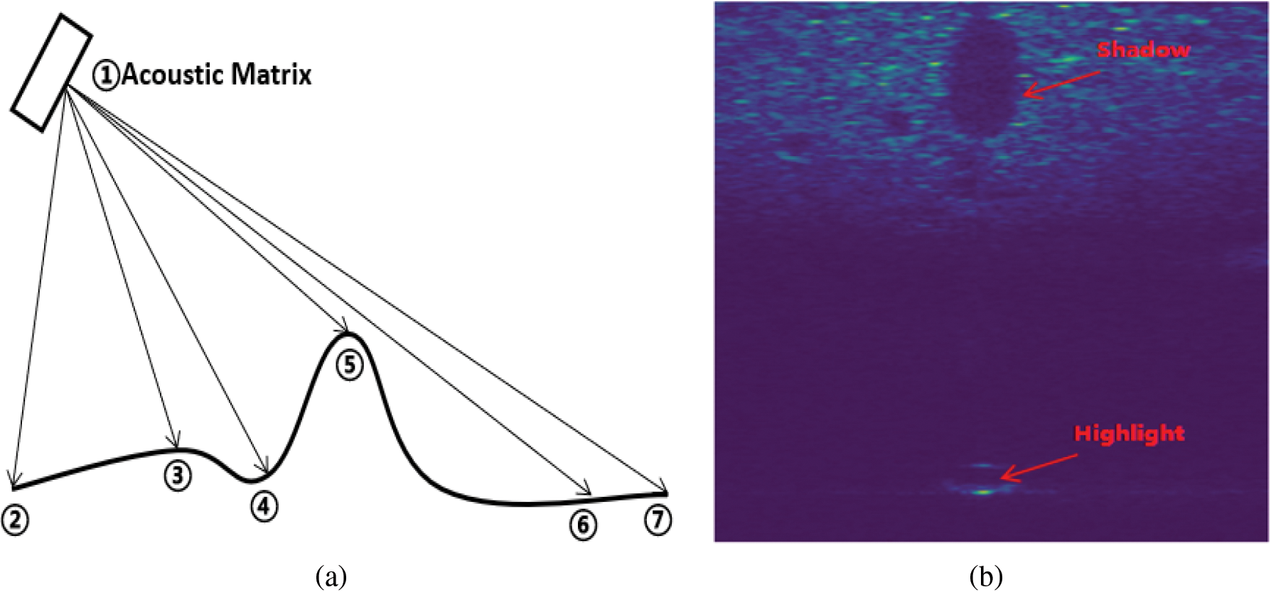
Figure 1: Schematic diagram of forward looking sonar imaging principle: (a) emits acoustic signals; (b) highlights and shadows in sonar images

2.2 Acoustic Shadow Capture Module

An acoustic shadow associated with the target item forms exactly above the target object in the forward-looking sonar picture as a result of the imaging properties of the device. Traditional methods of capturing acoustic shadows rely mainly on human effort. Xiao et al. [36] proposed an acoustic shadow capture method for sonar images. The specific rules for acoustic shadow capture are as follows.

(1) Set up three parallel prediction convolutional layers for getting the target object position parameters θ(xc, yc, wobj, hobj). The highest score in the prediction box is selected here, where xc and yc denote the coordinates of the center point of the target object in the feature map, and wobj and hobj denote the width and height of the target object in the feature map.

(2) The coordinates of the upper left corner of the object are obtained from the position parameter of the object (x1, y1), then the height H of the acoustic shadow region is y1 − yL, and the width W is taken as the width of the target object wobj, where yL is the vertical coordinate 0 of the upper left corner pixel point of the feature map.

(3) Since the width of some of the acoustic shadows is slightly larger than the target object, and there is also a small offset of the acoustic shadows toward the left and right sides, a width parameter α is introduced. α is used to adjust the width of the acoustic shadow area. The final width of the acoustic shadow area should be α * wobj.

2.3 Feature Fusion Module

In target detection, fusing different scales of features is an important means to improve the performance of model detection. Concat and Add are two commonly used classical feature fusion methods. Concat directly splices two features, while add directly adds two features. SSD [25] is the first time to use multi-scale feature fusion to make predictions by extracting features of different scales. FPN [17] Fuses the results of the upper sampling with features of the same scale generated from the bottom up through a top-down up sampling process and a horizontally connected process. This approach effectively enhances the representation of features by utilizing both high-resolution information of low-level features and high-level features. Following the FPN, a number of characteristic pyramid models with similar top-down structures have emerged [37–40]. For example, PANet [41], creates a bottom-up path based on FPN, which alleviates the loss of shallow information in network transmission. However, these feature pyramid-based methods still have inconsistencies at different scales, which limits further performance gains. ASFF [35] learns the mapping relationship between different features by filtering conflict information spatially, which is more conducive for different scales of features and effectively alleviates this problem.

3  The Proposed Method

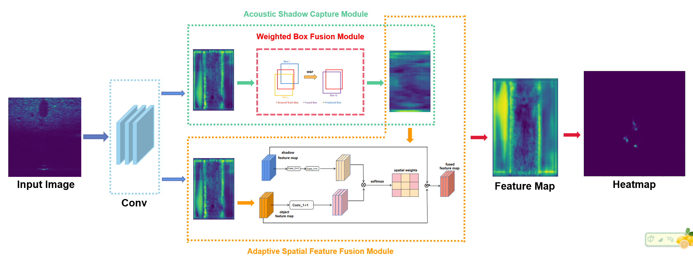
From above discussion, The existing mainstream methods do not make full use of the shadow information in sonar images, although it plays a vital role in the acquisition and recognition of target information in images. For the acoustic shadow capture module proposed by [36], the accuracy of the target object frame predicted by the model directly determines the accuracy of the acoustic shadow frame. However, they directly selected the target object prediction box with the highest score, ignoring the operation of other prediction boxes. Obviously, it is unreasonable because some prediction boxes with similar scores to the prediction box with the highest score can also well represent the location of the target object. Thus, we introduce a weighted box fusion (WBF) [42] method to fuse these prediction boxes and measure the contribution of each prediction box, and then generate an average box to obtain more accurate target object frames. Since traditional fusion methods, such as Add and Concat, simply fuse shadow information with the target object, and do not take into account the relative importance of shadow features and target object features, we adopt an adaptive spatial feature fusion strategy. By generating an adaptive normalized fusion weight, shadow information and target object are weighted and fused to make full use of acoustic shadow features. In addition, since the reason that regions with high fusion weight values contain important feature information, the model should pay more attention to these areas. On the contrary, regions with low fusion weight values contain unimportant feature information, which do not contribute to the model prediction, and may even have a negative impact on the model prediction. The model should be allowed to ignore these areas. Therefore, this paper proposes a threshold processing operation, which updates the generated fusion weight by setting a threshold gate, setting the higher fusion weight value to one and the lower fusion weight value to zero. The overall structure of the proposed target detection model is shown in Fig. 2, which will be described in detail in the following sections.

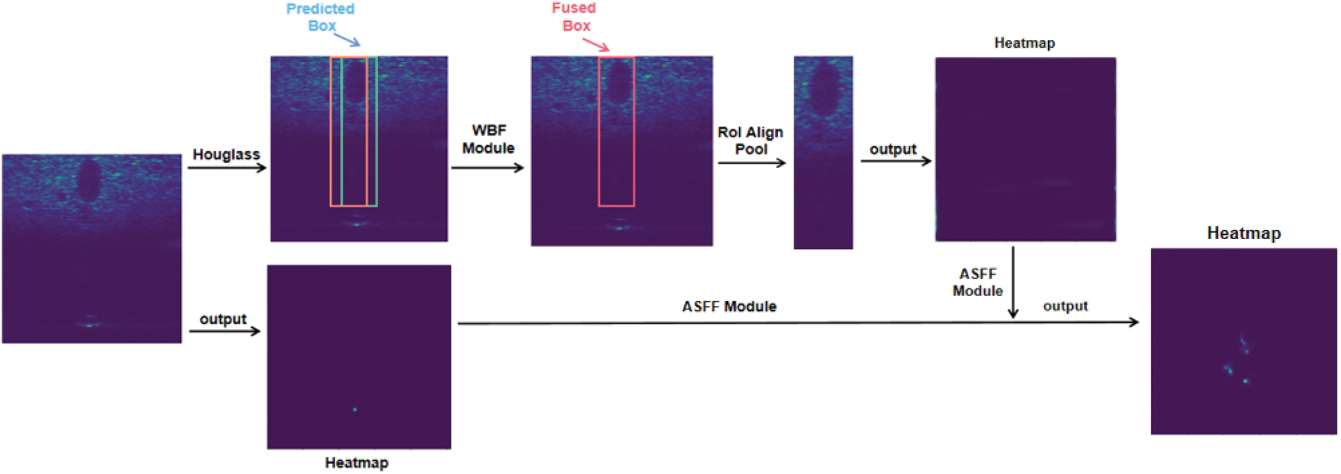
Figure 2: Acoustic shadow capture and fusion diagram

3.1 Weighted Box Fusion Module

In this section, we detail the weighted box fusion module [42]. The weighted frame fusion module considerably increases the accuracy of the prediction frame and the cut location of the acoustic shadow frame, which is similar to the secondary accuracy of the prediction frame provided by the model. By weighted fusion of the highly scored prediction frames, it is able to acquire a more precise acoustic shadow frame cut location, resulting in a cut-down image with richer and more comprehensive acoustic shadow information. Assuming that the target detection model generates N prediction frames for a sonar image, the process of weighted frame fusion algorithm can be divided into the following steps:

•   Add all the prediction boxes from the model output to a List A, and rank the prediction boxes from large to small by confidence level.

•   Create two empty Lists B and C. List B is used to store all the prediction boxes (including one or a group of prediction boxes) of each class in List A, and List C is used to store the fusion boxes (including only one fusion box) generated by all the prediction boxes of each class in List B.

•   Loop through the prediction box in List A and find the matching prediction box in List C. The matching here means that the Intersection over Union (IoU) ratio of the two boxes is greater than 0.55.

•   If no matching box is found, add this box to the end of List B and List C, and then continue traversing the next box in List A.

•   If the corresponding match box is found, add this box to the position corresponding to the match box in List B and List C, and then continue to traverse the next box in List A.

•   According to the T prediction boxes in the updated List B, recalculate the coordinates and confidence of the fusion box in List C. The calculation formula is as follows:

C=∑i=1TCiT(1)

X1,2=∑i=1TCi∗X1,2i∑i=1TCi(2)

Y1,2=∑i=1TCi∗Y1,2i∑i=1TCi(3)

where (XT1, YT1) is the upper left corner coordinate of the Tth prediction box. (XT2, YT2) is the lower right corner coordinate of the Tth prediction box, and CT is the confidence level of the Tth prediction box.

•   The confidence score of the prediction box in C is adjusted again after traversing List A, and the adjustment formula is as follows:

C=C∗min(T,N)N(4)

or

C=C∗TN(5)

For example, the BOX to be fused are BOX L and BOX I. The fused BOX is BOX G. Assuming that Box L and Box I are (XL1,YL1,XL2,YL2,CL) and (XI1,YI1,XI2,YI2,CI), respectively, the Box G after fusion is:

(XL1∗CL+XI1∗CICL+CI,YL1,CL+YI1∗CICL+CI,XL2∗CL+XI2∗CICL+CI,YL2∗CL+YI2∗CICL+CI,CL+CI2)(6)

Here we use the confidence level of the prediction box as the weight of the weighted fusion, and weighted the coordinates of the prediction box, resulting in a weighted fusion average box, as shown in Fig. 3. The average box fully considers the importance and contribution of each prediction box. For the prediction box with higher confidence, the greater the weighted fusion weight and contribution, the more the shape and position of the fusion box are biased towards the prediction box with higher weight.

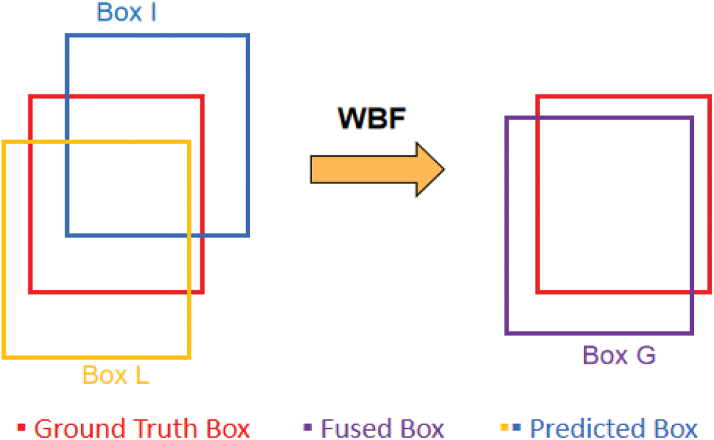
Figure 3: Weighted box fusion process

3.2 Adaptive Spatial Feature Fusion Module

In this section, the whole process of adaptive spatial feature fusion is introduced in detail. As shown in Fig. 4, ASFF can be divided into two steps of feature map scale adjustment and adaptive feature fusion. Unlike the traditional feature maps, which are directly added, spliced and cascaded with multi-scale features, ASFF achieves weighted fusion between feature maps by allowing different feature maps to learn an adaptive spatial feature fusion weight. The structure of the adaptive spatial feature fusion module is simple and effective, and the fusion is weighted according to the relative importance of acoustic shadow information and object target information, making the fusion more adequate and complete. As shown in Fig. 5, The adaptive spatial feature fusion module greatly enhances the adequacy of the fusion of acoustic shadow information and object target information.

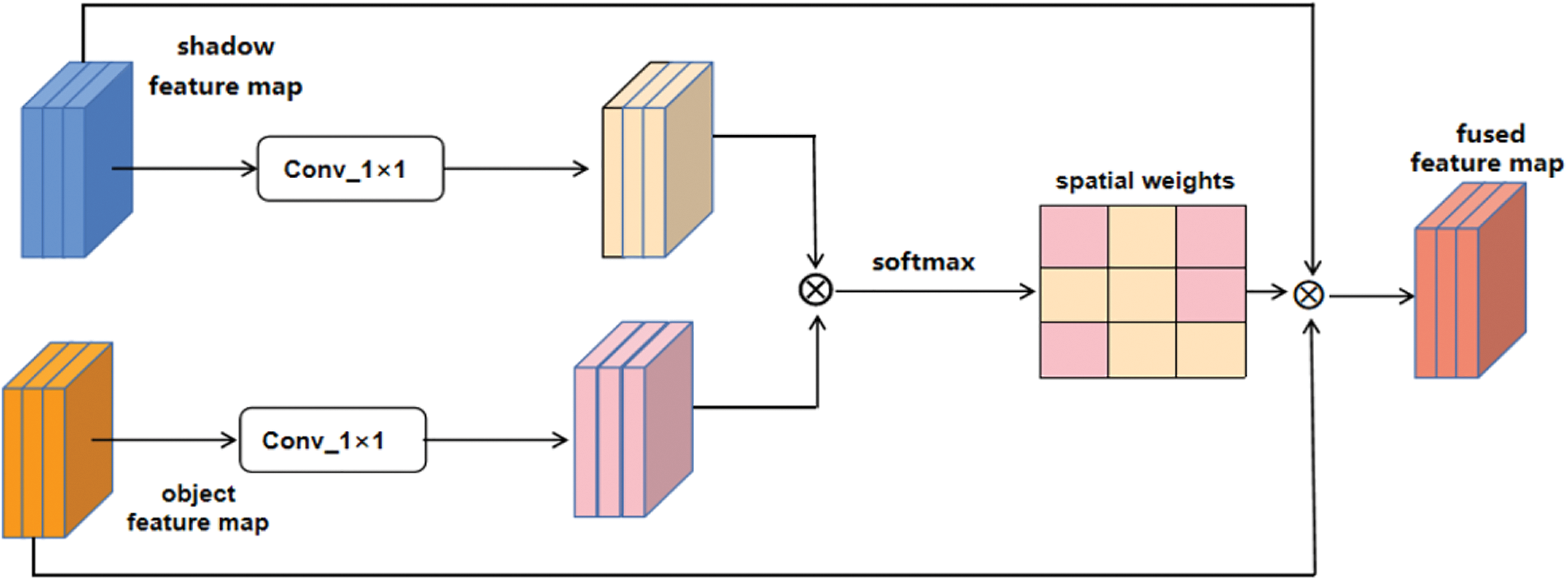
Figure 4: The structure of adaptive spatial feature fusion module. Acoustic shadow feature map captured and target object feature map are passed through 1 × 1 convolution is adjusted to the same size. Concat and Softmax function are used to generate spatial feature fusion weights. Finally, two feature maps are multiplied and added to generate fusion feature maps

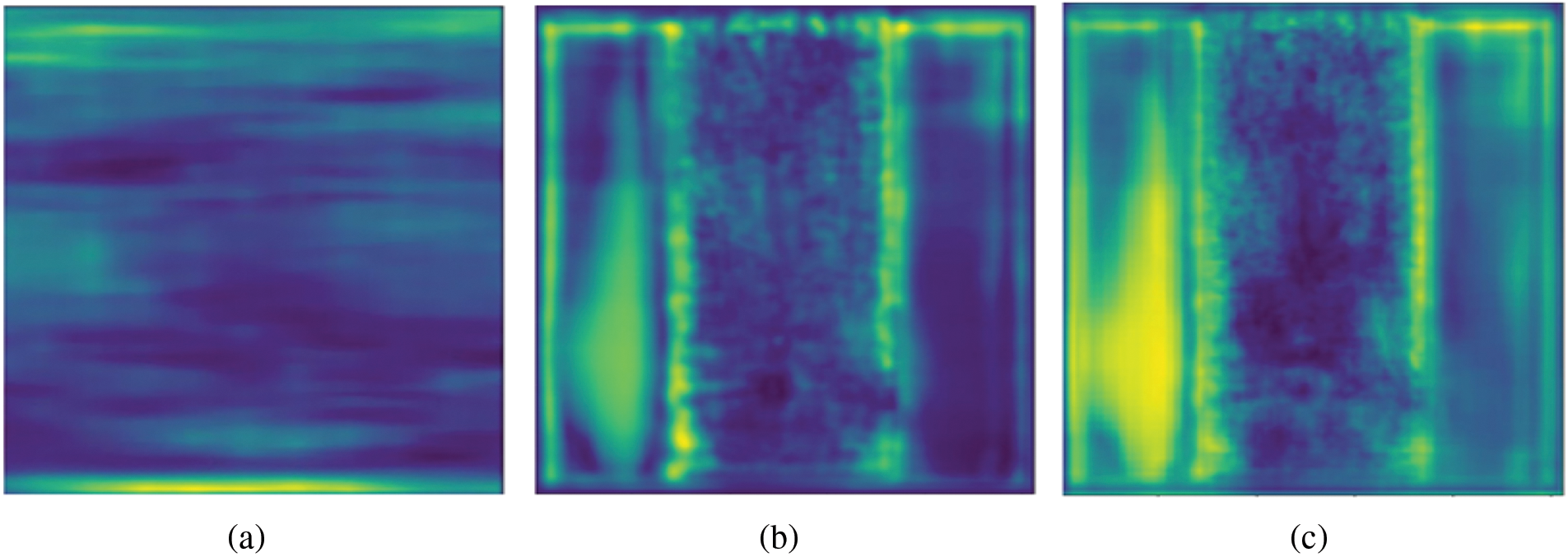
Figure 5: ASFF module heat map visualization which can be clearly observed that the fused images contain richer feature information: (a) thermogram of acoustic shadows cut off; (b) heat map of the target object; (c) thermal map after ASFF fusion

The size of the feature map that our model ultimately uses to predict is l (256 × 128 × 128). Because the acoustic shadow feature maps have different resolution and different number of channels under each cutting, different feature scale adjustment strategies are used to ensure that the scale of the acoustic shadow feature maps and the target object feature maps are consistent. For acoustically shaded images, we used a convolution layer of 3 × 3 to change the resolution of the input image to 128 × 128, and then compressed the channel number of the feature map to 256 through a convolution layer of 1 × 1. For the target object feature map, only one convolution layer 1 × 1 is needed to compress the channel number to 256. The final output feature fusion is l, whose fusion formula is shown in formula (7):

yi,jl=αi,jl⋅xi,j1→l+βi,jl⋅xi,j2→l(7)

where xi,jn→l represents the feature vector at the (i, j) position after adjusting the n-scale feature to the l-scale feature, yi,jl represents the vector after feature fusion at (i, j) position. αi,jl and βi,jl represent the fusion weights of the spatial features of different feature maps, respectively. They are learned adaptively by the network according to the feature information of different feature maps. The formula of fusion weight is defined as follows:

αi,jl=eλαi,jleλi,jl+eλβi,jl(8)

Among formula (8), the fusion weight parameters αi,jl and βi,jl are defined by using the softmax function with λαijl and λβijl as control parameters, respectively, to ensure that αi,jl + βi,jl=1 and αi,jl, βi,jl ∈ [0, 1].

3.3 Threshold Processing Module

The weights of the adaptive spatial feature fusion obtained in 3.2 are normalized. In places where the weight value is very small (such as less than 0.1), it can be considered that the features in this part will not have a great impact on the prediction of the model, even they may interfere with the prediction of the model as noise. Therefore, we directly set its weight value to 0, and let the model directly ignore this part of the characteristics. On the contrary, when the weight value is large (such as greater than 0.9), it can be considered that this part of the features are the most important features, which may directly determine the accuracy of the model prediction. For this, we directly set the weight value to 1, so that the model will pay more attention to this part of the features, as shown in Fig. 6.

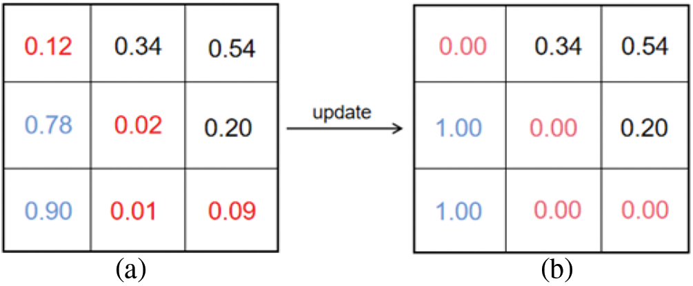
Figure 6: Threshold processing module example: (a) the fusion weights generated by ASFF; (b) the fusion weight after threshold module processing

4  Experimental Results and Analysis

In this section, we first make detailed experimental comparisons of the three proposed modules, discuss the impact of each module on the network, and then jointly study the role of the three modules on the entire network model. Under the evaluation standard of PASCAL VOC 2012, the proposed method achieved good performance improvement.

4.1 Dataset

In order to verify the validity and superiority of the proposed model, we carried out an experiment on the launch of an acoustic image data set in Pengcheng Laboratory. The data collection device is a Tritech Gemini 1200i multi-beam forward-looking sonar, and the data set is the original echo intensity information of the sonar in the form of a two-dimensional matrix. The storage format of the forward looking sonar image file is bmp, and the corresponding format annotation result file storage format is xml.

The data set contains 5000 images, including 3200 training sets, 800 verification sets and 1000 measurement sets. There are 8 target categories in total, including 3 types of regular geometric object cubes, spheres, cylinders and 5 types of underwater object mannequins, tires, round ground cages, square ground cages, and iron drums. The sample image of the dataset is shown in Fig. 7. The original sonar image is directly displayed as an image close to full black without gain adjustment, as shown in Fig. 7a. After histogram equalization of data, a more intuitive display effect can be obtained as shown in Fig. 7b, where the box contains the target area, and the target categories are the square cage, tyre, and ball from left to right.

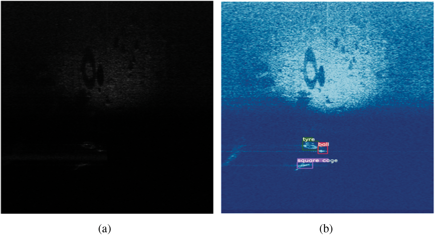
Figure 7: Sonar image data collection example: (a) original sonar image without gain adjustment; (b) after histogram equalization of (a)

4.2 Assessment Indicators

To measure and compare the detection performance of the proposed method, the performance metrics IoU, Precision, Recall, AP and mAP are used. IoU is a measure based on the Jackard index, which is used to evaluate the overlap between two bounding boxes. The IoU size can be used to determine whether the detection is valid or invalid. For a real bounding box A and a predicted bounding box B, IoU is equal to the overlapping area between them divided by the union area between them. The calculation formula of IoU is as follows:

IoU(A,B)=A∩BA∪B(9)

Precision represents the proportion of positive samples among all the predicted positive samples, which can evaluate the model’s ability to identify related objects. Recall indicates the proportion of positive samples predicted in the actual positive samples, which can evaluate the model’s ability to find all relevant cases. The calculation formulas of Precision and recall are shown in formulas (10) and (11), respectively.

Precision=TPTP+FP(10)

Recall=TPTP+FN(11)

where TP (true example) and TN (true counterexample) respectively represent positive samples and negative samples predicted by the model as positive classes, FP (false positive example) and FN (false counterexample) respectively represent negative samples predicted by the model as positive classes and positive samples of negative classes. When we take different confidence levels, a set of precision and recall values can be obtained and the curves they plot are called P-R curves. Define AP to calculate the area under a specific type of P-R curve, and define mAP to calculate the average area of all categories of P-R curves. Then AP represents the average detection accuracy of a single target category, and mAP represents the average value of multiple target categories. AP and mAP reflect the performance of the whole model, and their calculation formulas are shown in formulas (12) and (13), respectively:

AP=∫01P(R)dt(12)

mAP=∑n=0NAPn/N(13)

where N represents the number of target categories.

4.3 Parameter Settings

The backbone network we selected is Houlass, and the input image size of the model in the training phase is 512 × 512, the size of the output image is 128 × 128, the batch size is 8, and the basic learning rate is set to 0.001. The training strategy of constant step size decline of learning rate is adopted. Each time the learning rate drops to 1/10 of the original, the number of descending rounds is 120, 200 and 260, respectively, and the number of training rounds is 300. The verification is conducted every 5 training rounds.

4.4 Experimental Comparison

In order to verify whether the WBF module enables the model to obtain a more accurate acoustic shadow box, it is compared with the benchmark model under the PASCAL VOC2012 evaluation standard. We compared various categories of AP and mAP under different IoU, and visualized the output results of the modules. The precision performance and module visualization results under different IoU are shown in Tables 1, 2 and Fig. 8. It can be seen from Table 2 that when the WBF module is added, the mAP of the model is 97.17%, 90.28%, 75.06% and 26.75% respectively when the IoU is 0.5, 0.6, 0.7 and 0.8. In particular, when the IoU is 0.7, the mAP of the model is increased by 0.86%, while when the IoU is 0.8, the mAP of the model is increased by 2.82%. From the visualization results shown in Fig. 8, it can be clearly observed that after the WBF module is added to the model, more accurate acoustic shadow boxes are obtained, more complete acoustic shadows are cut down, and more abundant semantic information is obtained, which is precisely why the accuracy of the model is improved.

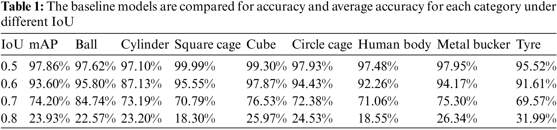
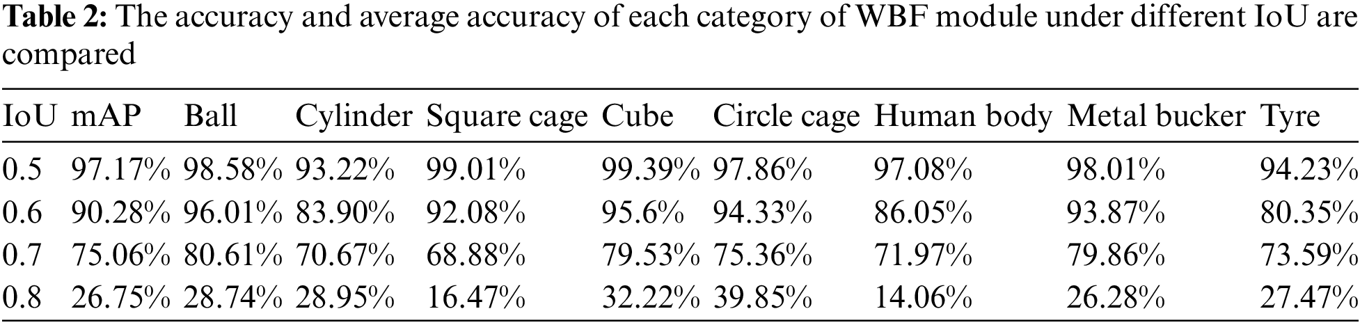
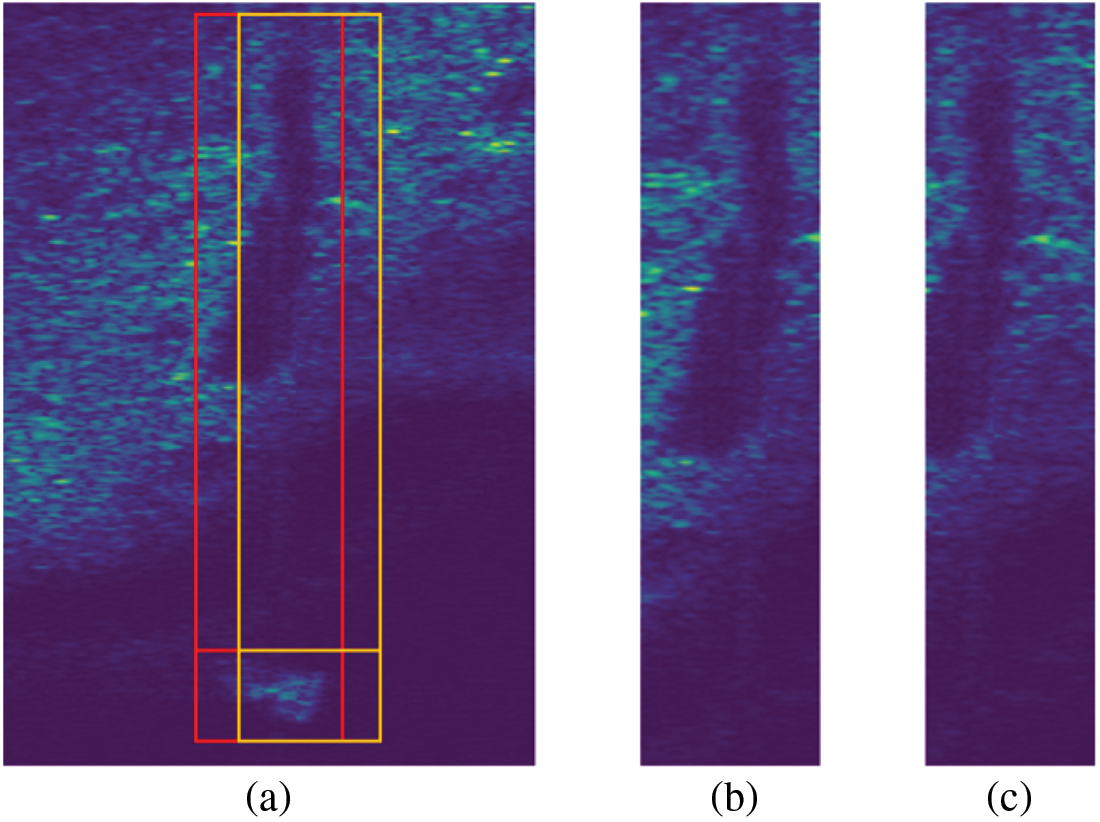
Figure 8: WBF module compared with the acoustic shadow box obtained from the reference model: (a) the red box is the acoustic shadow box obtained by the WBF module, and the yellow box is the acoustic shadow box obtained by the reference model; (b) acoustic shadows cut off by our model; (c) acoustic shadows from the final cut of the reference model

To verify whether the ASFF module enables the proposed method to obtain more sufficient semantic information, we compared it with the benchmark model under the PASCAL VOC2012 evaluation standard. We compare the AP and mAP of each category under different IoUs, and visualize the output of the module for the heat map. The precision performance and module visualization results under different IoUs are shown in Table 3 and Fig. 9. It can be seen from Table 3 that after adding the ASFF module, when IoU is 0.5, 0.6, 0.7 and 0.8, the mAP of the model is 98.15%, 92.80%, 75.31% and 22.37%, respectively. In particular, when IoU is 0.5, the mAP of the model is increased by 0.29%, and when IoU is 0.7, the mAP of the model is increased by 1.11%. It can be clearly observed in the visual heat map shown in Fig. 9 that after ASFF module fusion, the model outputs more highlighted reaction areas of the heat map, which means that the model has obtained more sufficient semantic information, thus further improving the detection accuracy.

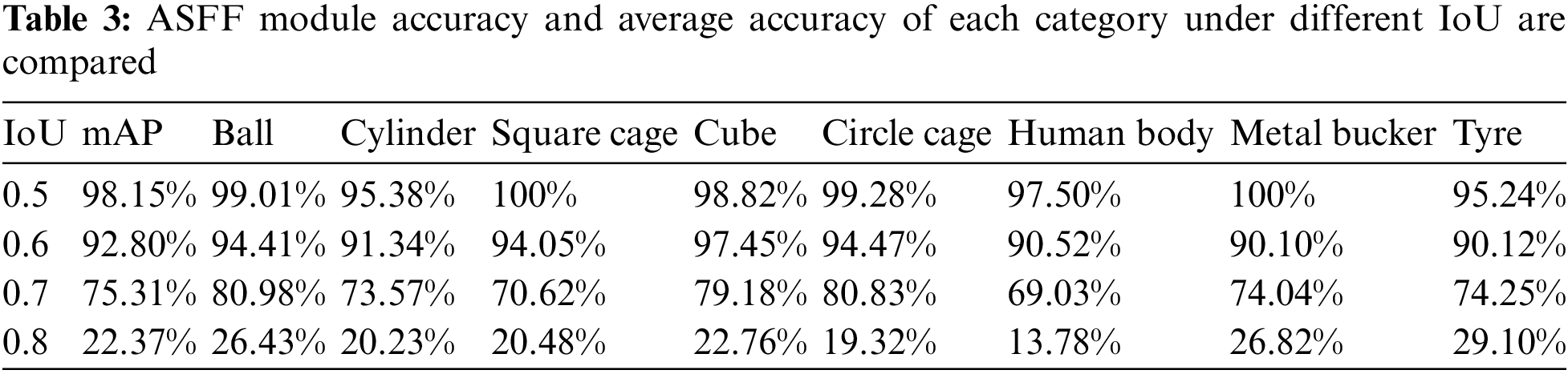
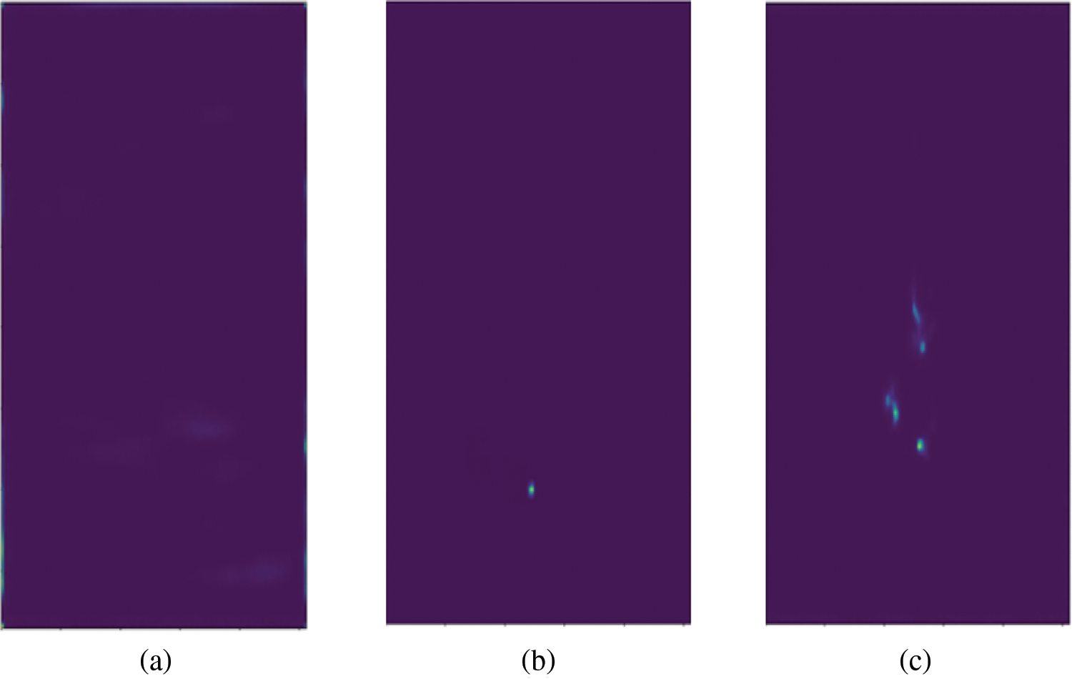
Figure 9: By comparing the heat maps of model output before and after ASFF fusion, the more highlighted reaction areas in the graph, the more important information the model focuses on: (a) acoustic shadow thermogram under cutting; (b) heat map of model output before ASFF fusion; (c) heat map of model output after ASFF fusion

Furthermore, this paper discussed in detail the impact of the three modules on the proposed model under the IoU of 0.7. Under the PASCAL VOC2012 evaluation standard, we compare each category of AP and mAP with the benchmark model for the model with three modules. The precision performance of the three modules and the benchmark model under the IoU of 0.7 is shown in Tables 4 and 5. Table 4 shows that when the IoU is 0.7, the mAP of the benchmark model is 74.20%, that of the model with the WBF module is 75.06%, that of the model with the ASFF module is 75.31%, and that of the model with threshold module is 75.73%. Finally, the mAP of the proposed model is 77.33%, which is 3.14% higher than that of the benchmark model. In addition, we also evaluated the accuracy change of the model after adding each module in detail. It can be observed from Table 5 that the accuracy of the model has been improved by the three modules we proposed, which verifies the effectiveness of each module.

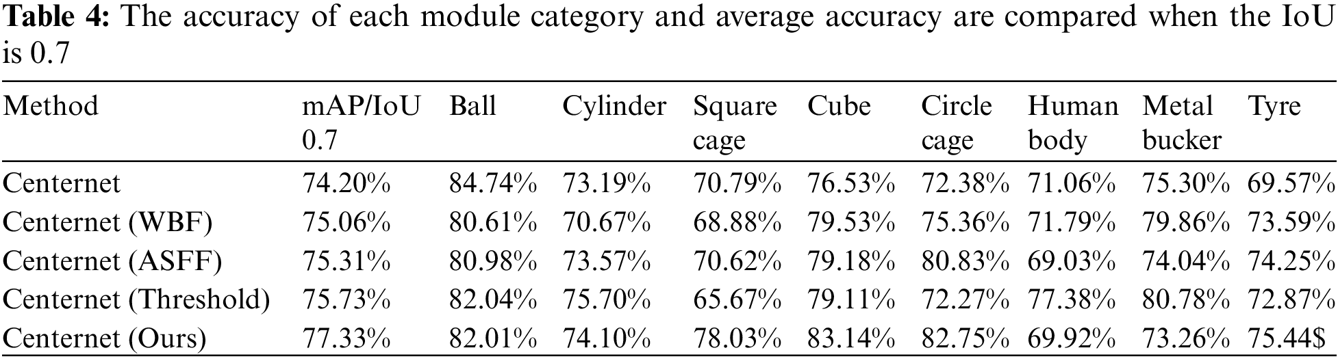
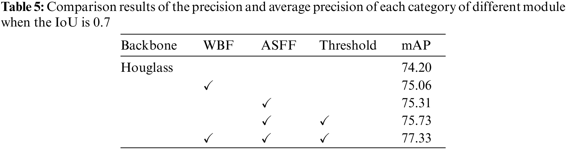
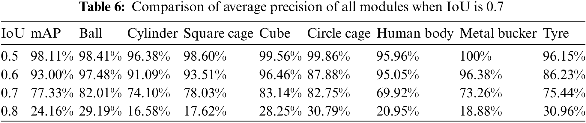
Table 6 shows the mAP of each category of the proposed model under different IoU under the PASCAL VOC2012 evaluation standard. It can be seen that when IoU is 0.5, 0.6, 0.7 and 0.8, the mAP of the proposed model is 98.11%, 93.00%, 77.33% and 24.16%, respectively. Compared with the baseline model, the mAP of the proposed model is improved by 0.25% when IoU is 0.5, and the mAP of the proposed model is almost unchanged when IoU is 0.6. When IoU is 0.7 and 0.8, the mAP of the model is increased by 3.14% and 0.23%, respectively. It is not difficult to draw a conclusion that the proposed model achieves good performance under each IoU. The accuracy of the proposed model is improved because it fully integrates the information of acoustic shadows and obtains more sufficient semantic information, which makes up for the feature information lost in sonar images due to the harsh underwater environment.

Finally, we compared the proposed model with various classical target detection models. The results are shown in Table 7. It can be found that the proposed model performs best in average accuracy. Meanwhile, for an IoU of 0.7, the detection results of this model are shown in Fig. 10. It can be observed that the model has a good recognition effect on sonar images of different categories, and there are no missed detections or false alarms. The specific detection results are as follows: In Fig. 10a, two objects of cylinder and circle cage were detected, with accuracies of 82% and 79%, respectively; in Fig. 10b, one object of cube was detected with an accuracy of 85%; and in Fig. 10c, three objects of square cage, tyre and cube were detected, with accuracy of 84%, 77% and 87%, respectively. The results of detection further verify that the model proposed in this paper has excellent performance for sonar image detection.

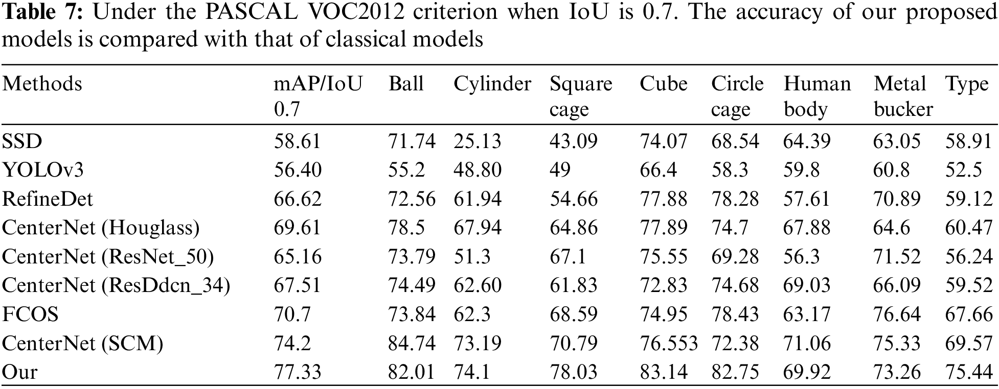
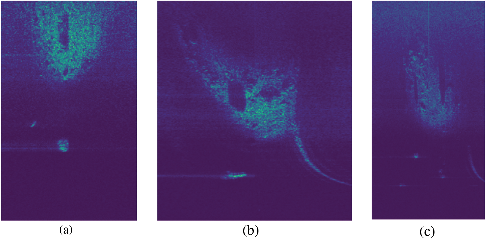
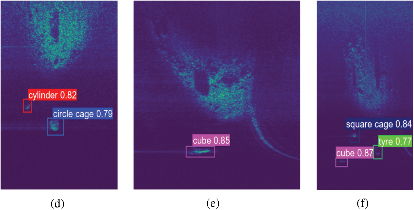
Figure 10: Different sonar images and their corresponding detection results

5  Conclusions

As green and renewable energy, ocean resources have great development potential and application value. By referring to the idea of the Internet of Things, the active and passive sonar systems and multi platform acoustic sensors are integrated into the Internet, so that the sonar in the network can switch and complement each other at any time, and then a multi base and multi azimuth integrated intelligent sonar system can be built to develop marine resources and monitor the marine environment. In this paper, we discussed some problems of forward-looking sonar in the field of underwater exploration and detection, and proposed a more effective and robust sonar image target detection framework based on deep learning to solve these problems, which enriches sonar image feature information by capturing and fusing sound shadows. The proposed detection model integrates the weighted frame to obtain a more accurate acoustic shadow position, and the adaptive feature space fusion module is used to more fully integrate the acoustic shadow features into the feature map. In addition, the threshold processing of fusion weight is added to make the network pay more attention to important feature information. The final output feature map of the model contains richer semantic information, which enhances the feature recognition ability of the network. The validity of the proposed modules was also verified in subsequent experiments. The average accuracy of the models was improved by 3.14% when the three modules were combined.

Funding Statement: This work is supported by National Natural Science Foundation of China (Grant: 62272109).

Conflicts of Interest: The authors declare that they have no conflicts of interest to report regarding the present study.

References

1. Fei, T. A., Kraus, D., Zoubir, A. (2015). Contributions to automatic target recognition systems for underwater mine classification. IEEE Transactions on Geoscience and Remote Sensing, 53(1), 505–518. https://doi.org/10.1109/TGRS.2014.2324971 [Google Scholar] [CrossRef]

2. Chen, Q., Huang, M., Wang, H., Xu, G. (2022). A feature discretization method based on fuzzy rough sets for high-resolution remote sensing big data under linear spectral model. IEEE Transactions on Fuzzy Systems, 30(5), 1328–1342. https://doi.org/10.1109/TFUZZ.2021.3058020 [Google Scholar] [CrossRef]

3. Chen, Q., Huang, M., Wang, H. (2021). A feature discretization method for classification of high-resolution remote sensing images in coastal areas. IEEE Transactions on Geoscience and Remote Sensing, 59(10), 8584–8598. https://doi.org/10.1109/TGRS.2020.3016526 [Google Scholar] [CrossRef]

4. Wang, H., Xu, L. G., Yan, Z. Q., Gulliver, T. A. (2021). Low complexity MIMO-FBMC sparse channel parameter estimation for industrial big data communications. IEEE Transactions on Industrial Informatics, 17(5), 3422–3430. https://doi.org/10.1109/TII.2020.2995598 [Google Scholar] [CrossRef]

5. Li, J. W., Jiang, P., Zhu, H. (2021). A local region-based level set method with markov random field for side-scan sonar image multi-level segmentation. IEEE Sensors Journal, 21(1), 510–519. https://doi.org/10.1109/JSEN.2020.3013649 [Google Scholar] [CrossRef]

6. Greene, A., Rahman, A. F., Kline, R., Rahman, M. S. (2018). Side scan sonar: A cost-efficient alternative method for measuring seagrass cover in shallow environments. Estuarine Coastal and Shelf Science, 207(4), 250–258. https://doi.org/10.1016/j.ecss.2018.04.017 [Google Scholar] [CrossRef]

7. Tueller, P., Kastner, R., Diamant, R. (2020). Target detection using features for sonar images. IET Radar, Sonar & Navigation, 14(12), 1940–1949. https://doi.org/10.1049/iet-rsn.2020.0224 [Google Scholar] [CrossRef]

8. Klausner, N. H., Azimi-Sadjadi, M. R. (2020). Performance prediction and estimation for underwater target detection using multichannel sonar. IEEE Journal of Oceanic Engineering, 45(2), 534–546. https://doi.org/10.1109/JOE.2018.2881527 [Google Scholar] [CrossRef]

9. Lee, D. H., Shin, J. W., Do, D. W., Choi, S. M., Kim, H. N. (2019). Robust LFM target detection in wideband sonar systems. IEEE Transactions on Aerospace and Electronic Systems, 53(5), 2399–2412. https://doi.org/10.1109/TAES.2017.2696318 [Google Scholar] [CrossRef]

10. Wang, H., Xiao, P. P., Li, X. W. (2022). Channel parameter estimation of mmWave MIMO system in urban traffic scene: A training channel based method. IEEE Transations on Intelligent Transportation Systems, 1–9. https://doi.org/10.1109/TITS.2022.3145363 [Google Scholar] [CrossRef]

11. Chen, Q., Ding, W., Huang, X., Wang, H. (2022). Generalized interval type II fuzzy rough model based feature discretization for mixed pixels. IEEE Transactions on Fuzzy Systems, 31(3), 845–859. https://doi.org/10.1109/TFUZZ.2022.3190625 [Google Scholar] [CrossRef]

12. Baussard, A., Acremont, A., Quin, G., Fablet, R. (2020). Faster-RCNN with a compact CNN backbone for target detection in infrared images. SPIE Proceeding. In: Artificial intelligence and machine learning in defense applications, 11543. Strasbourg, France. [Google Scholar]

13. Yin, S., Li, H., Teng, L. (2020). Airport detection based on improved faster RCNN in large scale remote sensing images. Sensing and Imaging, 21(1), 1–13. https://doi.org/10.1007/s11220-020-00314-2 [Google Scholar] [CrossRef]

14. Hong, X., Yang, D., Sun, N., Chen, Z., Zhang, Y. (2019). Automated pulmonary nodule detection in CT images using deep convolutional neural networks. Pattern Recognition, 52, 109–119. [Google Scholar]

15. Dong, R., Xu, D., Zhao, J., Jiao, L., An, J. (2019). Sig-NMS-based faster R-CNN combining transfer learning for small target detection in VHR optical remote sensing imagery. IEEE Transactions on Geoscience and Remote Sensing, 57(11), 8534–8545. https://doi.org/10.1109/TGRS.2019.2921396 [Google Scholar] [CrossRef]

16. Lan, X., Zuo, Z. (2014). Random-valued impulse noise removal by the adaptive switching median detector and detail-preserving regularisation. Optik, 125(3), 1101–1105. https://doi.org/10.1016/j.ijleo.2013.07.114 [Google Scholar] [CrossRef]

17. Shan, Y., Zhou, X., Liu, S., Zhang, Y., Huang, K. et al. (2015). Siamd: A deep learning method for accurate and real-time maritime ship tracking. IEEE Transactions on Circuits and Systems for Video Technology, 31(1), 315–325. https://doi.org/10.1109/TCSVT.2020.2978194 [Google Scholar] [CrossRef]

18. Han, H. Y., Chen, Y. C., Hsiao, P. Y., Fu, L. C. (2021). Using channel-wiseattention for deep CNN based real-time semantic segmentation with class-aware edge information. IEEE Transactions on Intelligent Transportation Systems, 22(2), 1041–1051. https://doi.org/10.1109/TITS.2019.2962094 [Google Scholar] [CrossRef]

19. Ren, S., He, K., Girshick, R., Sun, J. (2015). Faster R-CNN: Towards real-time object detection with region proposal networks. Advances in Neural Information Processing Systems, 28, 91–99. [Google Scholar]

20. Girshick, R. (2020). Fast R-CNN. Proceedings of the IEEE International Conference on Computer Vision, pp. 1440–1448. Santiago, Chile. https://doi.org/10.1109/ICCV.2015.169 [Google Scholar] [CrossRef]

21. Girshick, R., Donahue, J., Darrell, T., Malik, J. (2016). Region-based convolutional networks for accurate object detection and segmentation. IEEE Transactions on Pattern Analysis and Machine Intelligence, 38(1), 142–158. https://doi.org/10.1109/TPAMI.2015.2437384 [Google Scholar] [PubMed] [CrossRef]

22. Redmon, J., Divvala, S., Girshick, R., Farhadi, A. (2016). You only look once: Unified, real-time object de-tection. Proceedings of the IEEE Conference on Computer Vision and Pattern Recognition, vol. 2, pp. 779–788. https://doi.org/10.1109/CVPR.2016.91 [Google Scholar] [CrossRef]

23. Redmon, J., Farhadi, A. (2017). YOLO9000: better, faster, stronger. Proceedings of the IEEE Conference on Computer Vision and Pattern Recognition, vol. 2, pp. 7263–7271. [Google Scholar]

24. Redmon, J., Farhadi, A. (2018). YOLOv3: An incremental improvement, vol. 4. arXiv preprint arXiv: 1804.02767. [Google Scholar]

25. Liu, W., Anguelov, D., Erhan, D., Reed, C. S., Fu, C. Y. (2016). SSD: Single shot multibox detector. Proceedings of the European Conference on Computer Vision, pp. 1–17. Amsterdam, Netherlands. https://doi.org/10.1007/978-3-319-46448-0_2 [Google Scholar] [CrossRef]

26. Lin, T. Y., Goyal, P., Girshick, R., He, K. M., Dollar, P. (2017). Focal loss for dense object detection. Proceedings of the IEEE International Conference on Computer Vision, 11(13), 2980–2988. https://doi.org/10.1109/ICCV.2017.324 [Google Scholar] [CrossRef]

27. Law, H., Deng, J. (2020). CornerNet: Detecting objects as paired keypoints. International Journal of Computer Vision, 128(3), 626–642. https://doi.org/10.1007/s11263-019-01204-1 [Google Scholar] [CrossRef]

28. Duan, K. W., Bai, S., Xie, L. X., Qi, H. G., Huang, Q. M. et al. (2019). CenterNet: Keypoint triplets forobject detection. Proceedings of the IEEE International Conference on Computer Vision, vol. 2, pp. 6569–6578. [Google Scholar]

29. Tian, Z., Shen, C. H., Chen, H., He, T. (2019). FCOS: Fully convolutional one-stage object detection. 2019 IEEE/CVF International Conference on Computer Vision(ICCV), pp. 9627–9636. Seoul, Korea (South). https://doi.org/10.1109/ICCV.2019.00972 [Google Scholar] [CrossRef]

30. Williams, D. P. (2016). Underwater target classification in synthetic aperture sonar imagery using deep convolutional neural networks. 2016 23rd International Conference on Pattern Recognition (ICPR), pp. 2497–2502.Cancun, Mexico. https://doi.org/10.1109/ICPR.2016.7900011 [Google Scholar] [CrossRef]

31. Zhou, T. (2022). Automatic detection of underwater small targets using forward-looking sonar images. IEEE Transactions on Geoscience and Remote Sensing, 60, 1–12. https://doi.org/10.1109/TGRS.2022.3181417 [Google Scholar] [CrossRef]

32. Wang, Z. (2022). Sonar image target detection based on adaptive global feature enhancement network. IEEE Sensors Journal, 22(2), 1–151. [Google Scholar]

33. Tucker, J. D. (2011). Coherence-based underwater target detection from multiple disparate sonar platforms. IEEE Journal of Oceanic Engineering, 36(1), 37–51. https://doi.org/10.1109/JOE.2010.2094230 [Google Scholar] [CrossRef]

34. Kong, W. Z., Hong, J. C., Jia, M. Y. (2020). YOLOv3-DPFIN: A dual-path feature fusion neural network for robust real-time sonar target detection. IEEE Sensors Journal, 20(7), 3745–3756. https://doi.org/10.1109/JSEN.2019.2960796 [Google Scholar] [CrossRef]

35. Liu, S., Huang, D., Wang, Y. (2019). Learning spatial fusion for single-shot object detection. arXiv preprint arXiv:1911.09516. [Google Scholar]

36. Xiao, T. W., Cai, Z. J., Lin, C., Chen, Q. (2021). A shadow capture deep neural network for underwater forward-looking sonar image detection. Mobile Information Systems, 12(1), 1–11. https://doi.org/10.1155/2021/3168464 [Google Scholar] [CrossRef]

37. Fu, C. Y., Liu, W., Ranga, A., Tyagi, A. (2017). DSSD: Deconvolutional single shotdetector. arXiv preprint arXiv:1701.06659. [Google Scholar]

38. Kong, T., Sun, F. C., Yao, A., Liu, H. P., Lu, M. et al. (2017). Ron: Reverse connection with objectnessprior networks for object detection. 2017 IEEE Conference on Computer Vision and Pattern Recognition (CVPR), pp. 5244–5252. Honolulu, HI, USA. https://doi.org/10.1109/CVPR.2017.557 [Google Scholar] [CrossRef]

39. Woo, S. Y., Hwang, S. (2018). Stair-Net: Top-down semantic aggregation for accurate one shot detection. 2018 IEEE Winter Conference on Applications of Computer Vision (WACV), pp. 1093–1102. Lake Tahoe, NV, USA. https://doi.org/10.1109/WACV.2018.00125 [Google Scholar] [CrossRef]

40. Zhang, S. F., Wen, L. Y., Bian, X., Lei, Z., Li, S. Z. (2018). Single-shot refinement neural network for object detection. 2018 IEEE/CVF Conference on Computer Vision and Pattern Recognition, pp. 4203–4212. Salt Lake City, UT, USA. https://doi.org/10.1109/CVPR.2018.00442 [Google Scholar] [CrossRef]

41. He, K., Gkioxari, G., Dollar, P., Girshick, R. (2020). Mask RCNN. IEEE Transactions on Pattern Analysis and Machine Intelligence, 2, 386–397. [Google Scholar]

42. Wang, W. M., Gabruseva, T. (2021). Weighted boxes fusion: Ensembling boxes from different object detection models. arXiv preprint arXiv:1910.13302v3. [Google Scholar]