
 Submit a Paper
 Propose a Special lssue
 Open Access
ARTICLE
An Innovative Finite Element Geometric Modeling of Single-Layer Multi-Bead WAAMed Part
1 College of Mechanical and Power Engineering, China Three Gorges University, Yichang, 443002, China
2 School of Mechanical Science and Engineering, Huazhong University of Science and Technology, Wuhan, 430074, China
3 School of Metallurgy and Materials Engineering, Iran University of Science and Technology, Narmak, Iran
* Corresponding Authors: Xiangman Zhou. Email: ; Seyed Reza Elmi Hosseini. Email:
Computer Modeling in Engineering & Sciences 2024, 138(3), 2383-2401. https://doi.org/10.32604/cmes.2023.029249
Received 09 February 2023; Accepted 03 August 2023; Issue published 15 December 2023
 View Full Text
 Download PDF
Abstract
Finite element (FE) coupled thermal-mechanical analysis is widely used to predict the deformation and residual stress of wire arc additive manufacturing (WAAM) parts. In this study, an innovative single-layer multi-bead profile geometric modeling method through the isosceles trapezoid function is proposed to build the FE model of the WAAM process. Firstly, a straight-line model for overlapping beads based on the parabola function was established to calculate the optimal center distance. Then, the isosceles trapezoid-based profile was employed to replace the parabola profiles of the parabola-based overlapping model to establish an innovative isosceles trapezoid-based multi-bead overlapping geometric model. The rationality of the isosceles trapezoid-based overlapping model was confirmed by comparing the geometric deviation and the heat dissipation performance index of the two overlapping models. In addition, the FE-coupled thermal-mechanical analysis, as well as a comparative experiment of the single-layer eight-bead deposition process show that the simulation results of the above two models agree with the experimental results. At the same time, the proposed isosceles trapezoid-based overlapping models are all straight-line profiles, which can be divided into high-quality FE elements. It can improve the modeling efficiency and shorten the simulation calculation time. The innovative modeling method proposed in this study can provide an efficient and high-precision geometric modeling method for WAAM part FE coupled thermal-mechanical analysis.Keywords
Nomenclature
| An | Peak point of the Pn(x) profile |
| af | Length of the front ellipsoid of the heat source |
| ar | Length of the rear ellipsoid of the heat source |
| Bn | Intersection point between the tangent line of Pn(x) with Pn−1(x) |
| b | Width of the heat source |
| Cn | Intersection point of Pn(x) and Pn−1(x) |
| c | Depth of the heat source |
| Dn | Bottom point of the pipeline of the An |
| d | Overlapping center distance |
| En | Leftmost point of the Pn(x) |
| Fn | Rightmost point of the Pn(x) |
| ff | Fraction factor of the heat flux in the front parts |
| fr | Fraction factors of the heat flux in the rear parts |
| Gn | Left endpoint of Pn(x) in the overlapping gap of trapezoid-based model |
| Hn | Intersection point of GnIn and An−1Bn |
| h | Height of single bead |
| ht | Overlapping height of the isosceles trapezoid model |
| Id | Geometric deviation of the isosceles trapezoid-based overlapping model |
| In | Intersection points of Pn(x) and Pn−1(x) in the trapezoid-based overlapping model |
| IR(P) | Heat dissipation performance index of the parabola-based overlapping model |
| IR(T) | Heat dissipation performance index of the isosceles trapezoid-based overlapping model |
| Jn | Intersection point of InKn and An−1Bn |
| Kn | Right endpoint of Pn(x) in the overlapping gap of trapezoid-based model |
| Ln | Bottom point of the pipeline of the In |
| Pn(x) | Profile function of bead n |
| Q | Power input of FE model |
| w | Width of single bead |
| wt | Length of the upper side of the isosceles trapezoid model |
Wire arc additive manufacturing (WAAM) is a metal additive manufacturing (AM) technology that uses the electric arc as the heat source to melt the metal wire and add material layer by layer along the preset path [1]. Due to its high material deposition efficiency, high material utilization, direct full-density buildup properties, and potentially unlimited building volume, WAAM is generally considered the most promising rapid manufacturing technology for medium and large-scale components [2,3]. Therefore, WAAM technology has shown excellent application prospects in many fields, such as shipbuilding, transportation, aerospace, the nuke industry, and other frontiers [4].
However, the high material deposition efficiency of WAAM technology is caused by the high heat input that occurred in this process. Moreover, the moving heat source results in repeated localized heating and uneven cooling, which will lead to complex thermal cycles, distinctive local thermal gradients, and high residual stress in the WAAMed part. The high residual stress reduces the mechanical properties and geometric accuracy of the formed parts and even provokes pronounced distortions and cracks. This is considered one of the significant challenges of the WAAM process [5]. Therefore, the regulation and the control of the residual stress in the produced part are crucial to promote the extensive application of WAAM technology [6,7].
The finite element (FE) coupled thermo-mechanical analysis can reflect the transient thermodynamic information during the WAAM process in real time [8], which can provide internal details on distortion and residual stresses in the WAAMed part without considering the actual manufacturing process [9–11]. In particular, the dynamic thermal behavior, the evolution of stress, and distortion are analyzed to adjust the process parameters or select an optimal deposition strategy to formulate residual stress and deformation control strategies [12–15].
The geometric modeling of the deposition layer is essential for FE analysis. In most current studies, the cross-section profile of a single weld bead is usually simplified to a rectangle function. Sun et al. [16] and Köhler et al. [17] developed a rectangle cross-section-based FE model of a wire arc additive manufactured cuboid structure and studied the residual stress as well as the distortion of six different deposition strategies. Somashekara et al. [18] used the rectangle cross-section-based modeling method to establish the FE-coupled thermo-mechanical model for metallic additive manufacturing and investigated the effect of the weld-deposition pattern on residual stress evolution. Sun et al. [19] presented a unique pattern assessment criterion and constructed the FE-coupled thermo-mechanical model based on the rectangle cross-section model to evaluate and optimize the deposition mode. In addition, the curve fitting method is a standard method for modeling the cross-section profile of the weld bead. Zhao et al. [20] used the arc curve function to fit the outer profile of the deposited layer. They established the thermal-mechanical coupled finite element simulation model of the WAAM deposition process. The curve fitting method was also widely used to fit the section profile of the WAAM weld bead and calculate the optimal overlapping parameters [21]. However, the curve fitting function method has low efficiency for finite element modeling. Meanwhile, the rectangular section-based bead model is a wholly simplified model that produces a large sizable error in comparison to the actual weld bead. Zhan et al. [22] utilized an isosceles trapezoidal cross-sectional profile to replace the arc cross-sectional profile and established a single-bead finite element model for the laser melting deposition. The simulation results and the model deviation analysis show that the isosceles trapezoid-based model and the arc-based model have a minor deviation. In the meanwhile, the calculation efficiency of the trapezoid-based model is significantly improved.
In this study, to take into account both geometric accuracy and computational efficiency, an innovative single-layer multi-bead geometric modeling method based on the isosceles trapezoid function was proposed to establish the FE model of the WAAM process. Firstly, a straight-line overlapping model was selected based on a parabola function to calculate the optimal overlapping center distance. Then, a multi-bead isosceles trapezoid-based overlapping model was established based on the optimal center distance and the isosceles trapezoid model of a single bead. The comparisons of geometrical deviation and the heat dissipation performance index between two overlapping models were performed to verify the validity of the trapezoid-based overlapping model. In addition, the computational efficiency and error of the isosceles trapezoid-bead overlapping model were investigated through single-layer eight-bead deposition numerical simulation and corresponding experiment. The main innovations of this study are as follows: 1) A single-layer multi-bead overlapping model based on the isosceles trapezoid function was used to establish the finite element thermodynamic coupling simulation model of WAAM. 2) The proposed modeling method can provide a reference and technical idea for high efficiency and high precision modeling of WAAM finite element thermodynamic coupling simulation and other metal additive manufacturing technologies.
2 Straight-Line Overlapping Model Based on Parabola Function
2.1 Geometry of the Straight-Line Overlapping Model
During the FE analysis of the WAAM process, the accuracy of a geometric model is directly related to simulation accuracy and validity of the calculation results. Ding et al. [21] depicted that the parabola function, cosine function, and arc function can fit the weld bead profile with high accuracy. However, the parabola function is easier to compute than the cosine and arc functions. Herein, a straight-line overlapping model was built based on the parabola function to calculate the optimal overlapping center distance.
The principle of the straight-line overlapping model can be illustrated in Fig. 1. A parabola-based single-bead profile geometry model is established with the parameters of width (w) and height (h). The positive direction of the x-axis is the overlapping direction of multi-beads. According to the deposition order of weld beads, the profile function of the first bead is identified as P1(x). Analogously, the profile function of bead n is defined as Pn(x). The center distance of adjacent beads and the total width of beads are defined as d and W, respectively. Point E2 is the leftmost point of the P2(x) profile, and point B1 is a point on P1(x) profile, which shares the same abscissa with point E2. Point A2 is the peak point of the P2(x) profile and point C1 is the intersection of the P1(x) and P2(x) profiles. In this model, the curve of the transition area is assumed to be a straight line passing through points B1 and A2.
Figure 1: The multi-bead linear overlapping model
The first two bead functions are defined by Eqs. (1) and (2) as:
2.2 Optimal Center Distance of the Straight-Line Overlapping Model
The optimal overlapping center distance of the parabola-based single-bead profile geometry model is determined by the equal area criterion. As shown in Fig. 1, the coordinates of B1, C1, A2, E2, F1, and D2 are defined by
According to the ideal overlapping, the overlapping area of the two parabolas equals the area of the critical valley. According to this, the area
The curved-side triangle area
The function f(d) is expressed as Eq. (6).
When f(d) equals 0, the ideal overlapping condition is achieved. The two positive roots of equation f(d) = 0 is d1 = 3 w/4 = 0.75 w and
Figure 2: The schematic of the experimental setup
The cross-section profiles of the specimens are shown in Fig. 3. When the overlapping center distance is less than 0.75 w, the height of the second bead is greater than the first bead. When the overlapping center distance is greater than 0.75 w, the two weld beads have a similar size. The depth of the valley area between the two weld beads increases gradually with the increase of the overlapping center distance. If the center distance reaches 0.866 w, the depth of the valley area becomes deeper and results in poor flatness. Therefore, it can be seen that d = 0.75 w can be considered the optimal overlapping center distance.
Figure 3: The cross-section profiles of the specimens
3 The Isosceles Trapezoid-Based Overlapping Model Profile
3.1 Geometry of the Isosceles Trapezoid-Based Overlapping Model
In finite element geometric modeling of WAAM deposition layer, the cross-section profile of a single weld bead is usually simplified to a rectangle function or fitted by curvilinear equation (such as parabola function, cosine function, and arc function). However, the rectangle function method is an oversimplified method which is difficult to guarantee the accuracy of modeling and calculation. In the meantime, the curvilinear function method has high precision. However it has low efficiency for finite element geometric modeling, and it is difficult to partition into high-quality finite element mesh. Then, the isosceles trapezoid-based profile model is proposed to replace the parabola-based profile model in this study (as shown in Fig. 4). The red and black lines represent the profile of the isosceles trapezoid and parabola, respectively. To guarantee the equivalence, the parabola profile and the isosceles trapezoid profile are set to have the same length of the bottom side and height. Moreover, the two adjacent regions have the same area by controlling the length of the upper side, wt.
Figure 4: Schematics of the single bead cross-section
Eq. (7) represents two adjacent regions with the same area. Then, in the isosceles trapezoid-based model, the length of the upper side can be solved by Eq. (8).
Fig. 5 depicts the isosceles trapezoid-based overlapping model based on the isosceles trapezoid function and the optimal center distance. The red line represents the new weld bead profiles, and ht is the overlapping height of this innovative model.
Figure 5: Schematics of multi-bead isosceles trapezoid-based overlapping model
The area of the pentagon
To guarantee the equivalence, the cross-sectional area of the parabola model must be equal to the cross-sectional area of the isosceles trapezoid-based model. This means that the area of the pentagon
Consequently, ht value can be calculated by Eq. (11) as:
Then, ht = 0.6 h.
3.2 Rationality Analysis of the Isosceles Trapezoid-Based Overlapping Model
3.2.1 Geometrical Deviation Analysis
The parabola-based overlapping model is a fitting model with high accuracy. In contrast, the isosceles trapezoid-based overlapping model is a simplified model. Therefore, compared with the parabola-based model, the isosceles trapezoid-based model has a particular geometrical deviation. As shown in Eq. (12), the geometric deviation Id can be defined by the area of the non-overlapping area between the two models as:
where P(x) is the profile function of the parabolic-based overlapping model, and T(x) is the profile function isosceles trapezoid-based overlapping model. According to Eq. (12) and the geometric relationship in Fig. 5, the Id can be further expressed by Eq. (13).
The average geometric deviation id(n) of the single-bead model can be calculated by Eq. (14).
Eq. (14) illustrates that the average geometric deviation increases with the increase of the deposition beads. The maximum geometric deviation can be expressed by Eq. (15).
Previous researches [21,23–26] expressed that the ideal weld bead width satisfies w ∈ [4,12], and the bead height satisfies h ∈ [0, w/2]. Fig. 6 states the three-dimensional diagram and contour map of the average geometric deviation. According to Eq. (15) and Fig. 6, the average geometric deviation is positively correlated with the size of the bead. While the width (or height) of the bead remains constant, the greater the height (or width), the larger the average geometric deviation. Meanwhile, the maximum deviation is 3.6 mm2.
Figure 6: (a) Three-dimensional diagram and (b) contour map of average geometric deviation of one bead
Eq. (16) displays the quotient of the geometric deviation, which means the geometric consistency of the geometric model and actual weld bead. The parabola fitting model has high accuracy. Therefore, the parabola model is used to represent the natural weld bead in this study. Eq. (16) represents that the max average geometric deviation quotient of the isosceles trapezoid-based model is 7.5%. There is a high degree of geometric consistency between the isosceles trapezoid-based overlapping model and the parabolic-based overlapping model.
3.2.2 The Analysis of Heat Dissipation Performance Index
During the deposition process, the heat dissipation mechanism of the weld beads to the atmosphere includes convection and radiation. The heat dissipation performance index is directly related to the contact area between the beads and air [25]. Namely, the heat dissipation performance index of the beads can be represented by the surface area of the bead. The bead is assumed to have the same morphology along the welding direction. The calculation of relative surface area can be reasonably simplified from three-dimension to two-dimension. In other words, the heat dissipation area of the entire beads can be equivalent to the perimeter of the cross-section. Therefore, the heat dissipation performance index of the parabola-based overlapping model and isosceles trapezoid-based overlapping model can be expressed in Eqs. (17) and (18), respectively.
According to the geometric relationship in Figs. 1 and 5, IR(P) and IR(T) values can be expressed by Eqs. (19) and (20).
The error ID of the heat dissipation performance index can be defined by Eq. (21). This verifies the consistency of the heat dissipation performance index of the two models.
The three-dimensional diagram and contour map of the error of the heat dissipation performance index at n = 2 are shown in Fig. 7. The larger the height (or width), the greater the error of the heat dissipation performance index when the width (or height) of the bead remains constant. The maximum error is 7.2%.
Figure 7: (a) Three-dimensional diagram and (b) contour map of error percentage of heat dissipation performance index (n = 2)
The three-dimensional diagram and contour map of the error of the heat dissipation performance index at n ≥ 3 are shown in Fig. 8. When the bead height is less than 1.5 mm, the larger the height (or width), the greater the error of the heat dissipation performance index. Simultaneously, if the bead height exceeds 1.5 mm, the error decreases first and then increases with the increase of the bead width. When the bead width remains constant, the error decreases first and then increases with the rise in the bead height. The error of the heat dissipation performance index is 7.5%.
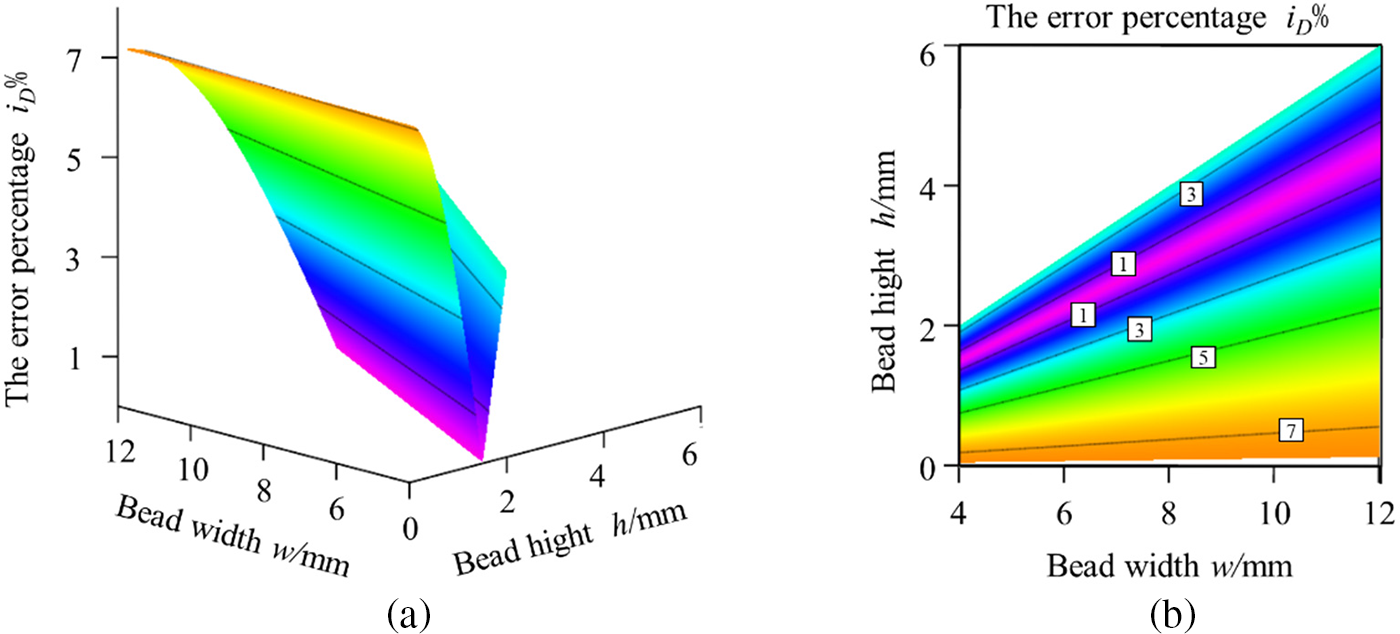
Figure 8: (a) Three-dimensional diagram and (b) contour map of error percentage of heat dissipation performance index (n ≥ 3)
To sum up, the geometric deviation and the error of heat dissipation performance index of the overlapping model between the isosceles trapezoid-based model and the parabolic-based model are less than 7.5%, which means that the overlapping modeling method based on the isosceles trapezoid function has acceptable accuracy error and is suitable for establishing the FE coupled thermal analysis model.
4 Verification of Single-Layer Multi-Bead FE Geometric Modeling Method Based on the Isosceles Trapezoid Function
4.1 Experiment Scheme and FE Analysis Model
To verify the validity of the proposed innovative FE geometric modeling method, a single-layer eight-bead deposition experiment and simulation are performed. Fig. 9 depicts the deposition direction and the size of the base metal.
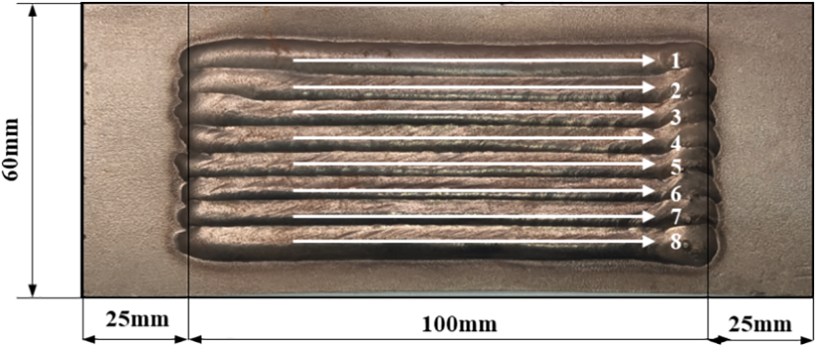
Figure 9: FEA model and deposition sequence
The single-layer eight-bead coupled thermo-mechanical models based on the isosceles trapezoidal and parabola functions are constructed in ABAQUS. The FE model is displayed in Fig. 10. In order to ensure the mesh quantity of the two models is consistent and avoid the calculation deviation due to the mesh quantity in the calculation results of the two models, the mesh of the beads and the substrate is divided by the controlling of the number of elements on the line and surface of the model. It can be seen that the mesh of the beads and the substrate is more uniform, which is conducive to improving the efficiency and accuracy of the FE calculation because all the lines of the isosceles trapezoid-based model are straight lines.
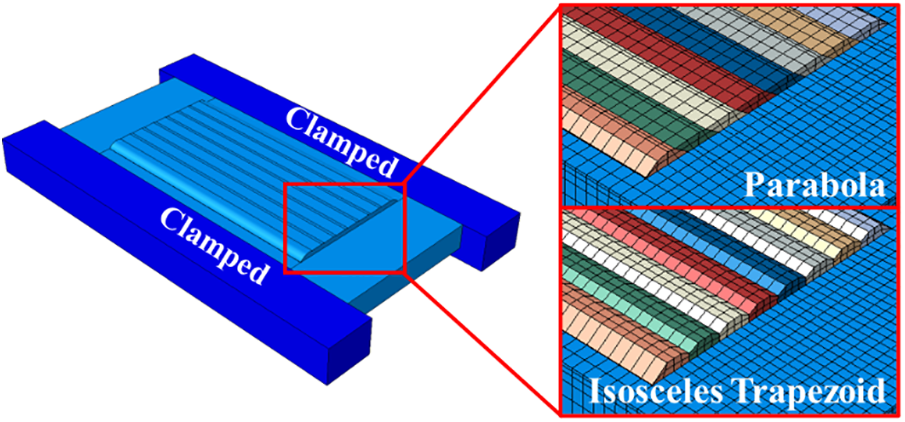
Figure 10: The meshing of the deposition beads and the substrate
As indicated in Eq. (22), the double ellipsoid heat source model is employed to describe the heat source distribution in the molten pool,
where b is the width of the heat source, c is the depth of the heat source, and af and ar are the length of the front and rear ellipsoid of the heat source, respectively. ff and fr are the fraction factors of the heat flux in the front and rear parts, respectively. Q is the power input. The source efficiency coefficient is 0.7 [13,24,25]. The temperature-dependent properties of the 304 stainless steel [27] are used in the simulation. The birth-death element method was employed to simulate the layer-by-layer deposition of the WAAM process. The deposition process, the heat source, and the boundary-condition-related parameters are listed in Tables 2–4, respectively. The heat source parameters are determined based on reference to previous similar studies and a comparison of numerical simulation and experimental results.
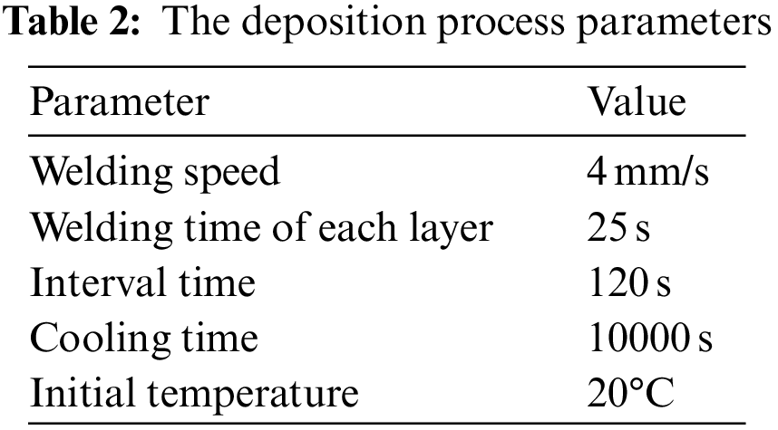
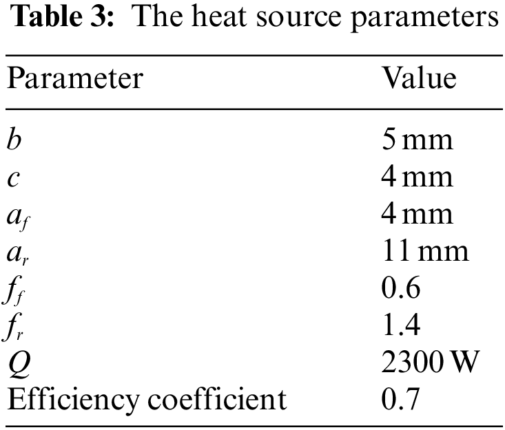
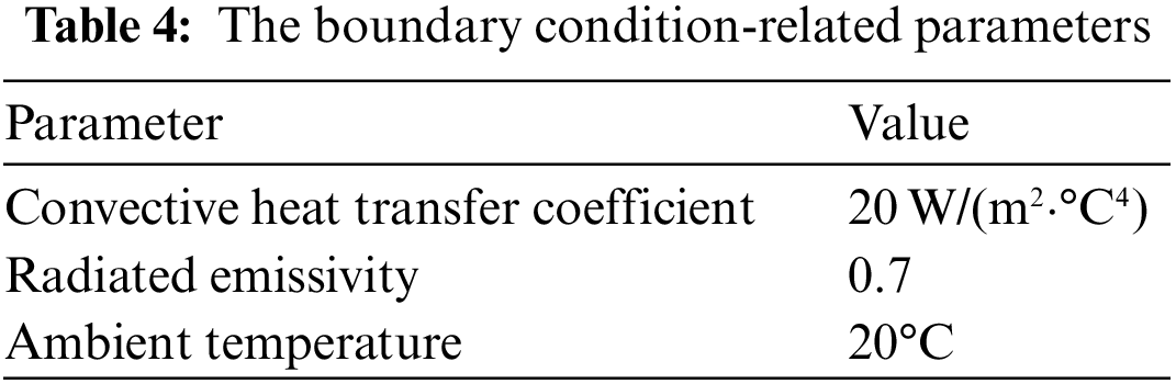
Fig. 11 shows the temperature contours of the finite element simulation of the two models at the end of the first, fourth, and eighth beads. It can be seen that the temperature distributions of the two models are close to each other at the end of each bead, and the peak temperature increases gradually with the increase in the number of deposition beads. The peak temperature of the parabolic-based model is 23°C higher than the isosceles trapezoid-based model. The peak temperature at the end of the fourth and eighth beads of the isosceles trapezoid-based model is slightly higher than the parabolic-based model (81°C and 19°C higher, respectively) except for the end of the first bead. It is because the depth of the ‘valley’ region between the two beads of the isosceles trapezoid-based model is deeper than the parabolic-based model (as shown in Fig. 5) that makes the heat more concentrated. Meanwhile, the heat dissipation performance index of the parabolic-based model is higher than the isosceles trapezoid-based model (as shown in Fig. 7), which means the heat diffusivity of the isosceles trapezoid-based model is slightly worse than the parabolic-based model. The temperature simulated result of the two models indicates that the two models have good consistency in temperature field simulation.
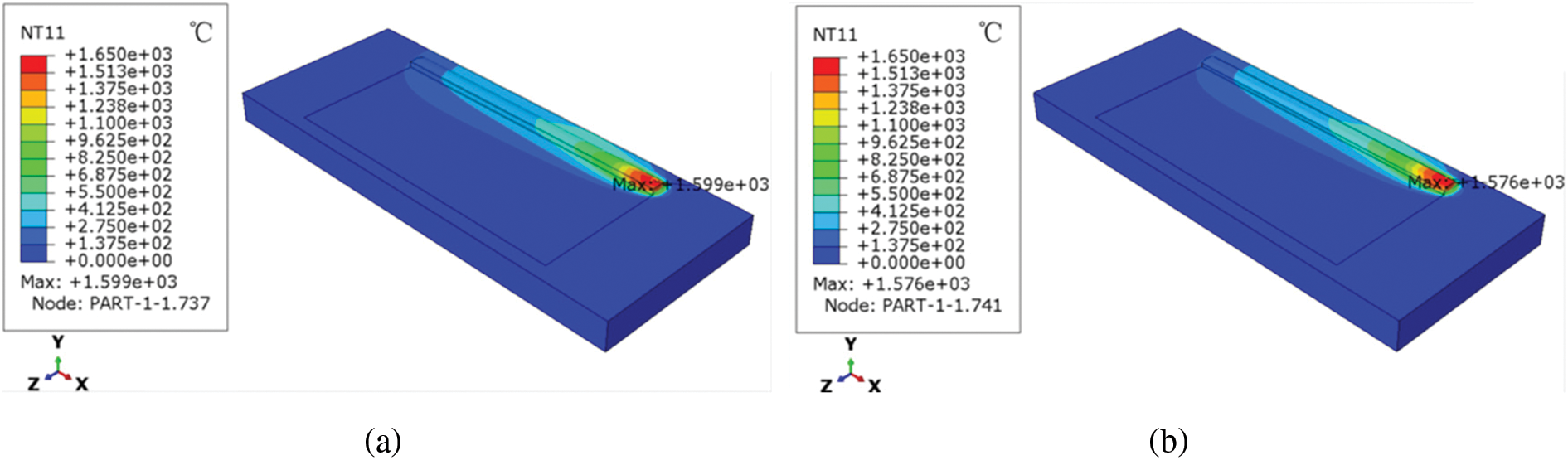
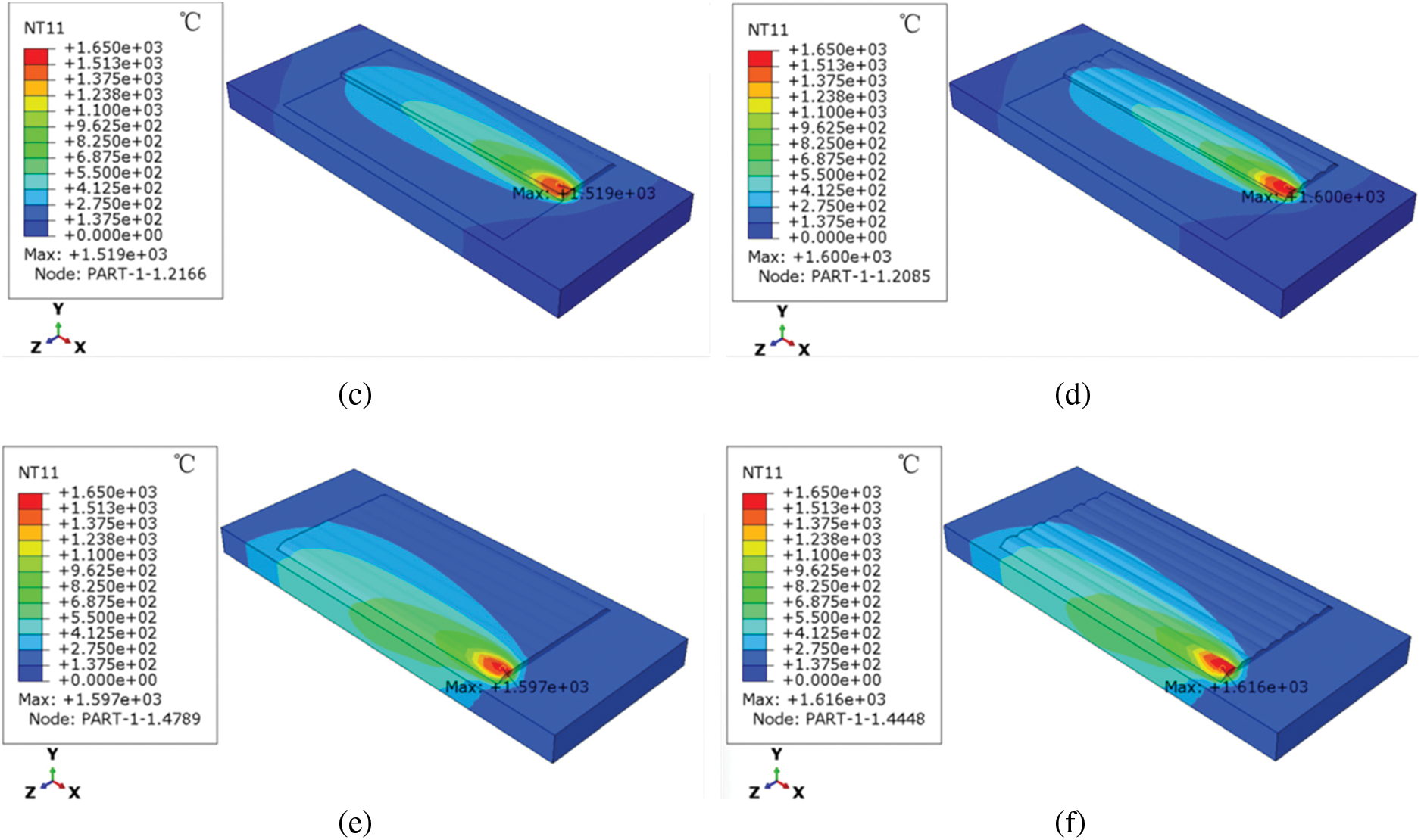
Figure 11: The temperature contours of FEM simulation of the two models at the end of the first, fourth, and eighth beads (a)∼(c) parabolic-based model, (d)∼(f) the isosceles trapezoid-based model
During the deposition experiment, a thermocouple sensor is set at point A (as shown in Figs. 2 and 12) on the substrate to measure the temperature cycle curve. During the simulation, the temperature value at point A is monitored in the simulation model. The thermal cycling curves of the simulation and experimental measurement at point A on the substrate are shown in Fig. 12. It depicts that all three thermal cycling curves have eight cycles. However, due to the short cooling time between the first two beads being close to each other at point A, there are two peak points at positions 1 and 2, as shown in Fig. 12, at the rising stage of the curves. The other six peak points at position 3 are close to each other. Among these the peaks in the simulation results are close to each other. The simulation and experimental results show that the simulated thermal cycles at the temperature of point A agree well with the measured results. This means that the two FE models are suitable for predicting thermal performance. The difference between the measured and simulated values is due to the model simplifying and measurement error. And there is a slight difference between the parabola and the trapezoidal models, which means that the isosceles trapezoid-based overlapping model and parabolic-based overlapping model have a high consistency.
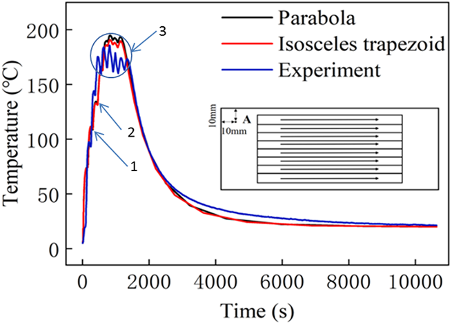
Figure 12: Simulated and experimental thermal cycles of point A
Fig. 13 shows the residual stress contours of the finite element simulation of the two models. It can be seen from Fig. 13 that the residual stress distribution laws obtained by the simulation of the two models are very similar, with only slight differences in local areas. This indicates that the two simulation models have good consistency in residual stress simulation.
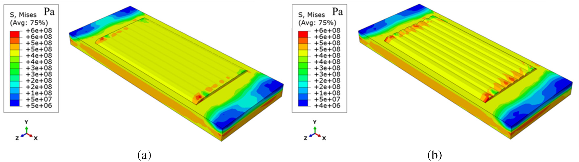
Figure 13: The residual stress contours of the FEM simulation (a) the parabolic-based model, (b) the isosceles trapezoid-based model
In order to verify the quantitative comparison results of the residual stress on the substrate obtained by the experiment and simulation, the residual stress values of four points on the substrate (as shown in Fig. 14) were measured by the XRD method. The residual stress values of four monitoring points at the same position were monitored in the simulation process to obtain the simulation results of the residual stress. Fig. 14 represents the measured and simulated residual stress of four points (Points 1, 2, 3, and 4) on the substrate. It can be seen from Fig. 14 that the measured residual stress values are matched with the simulation model at each point. The difference between the measured and simulated values is due to the model simplifying and measurement error. And there is a slight difference between the parabola and the trapezoidal models, which verify the consistency of the isosceles trapezoid-based and parabolic-based overlapping models.
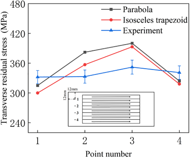
Figure 14: Comparison of the residual stress of two FE models with the experimental measurement result
The residual stress is extracted from paths on the surface of the substrate and bead to compare the residual stress simulation results of the two simulation models. Figs. 15a and 15b show the residual stress distribution on the CD and EF paths obtained from simulated results of the parabolic-based overlapping model and the isosceles trapezoid-based overlapping model, respectively. It can be seen from Fig. 15 that the distribution of residual stress is similar in both paths, and there is a slight difference in parts of the curves, which further verifies the consistency of the two models in the simulation results and the effectiveness of the isosceles trapezoid model.
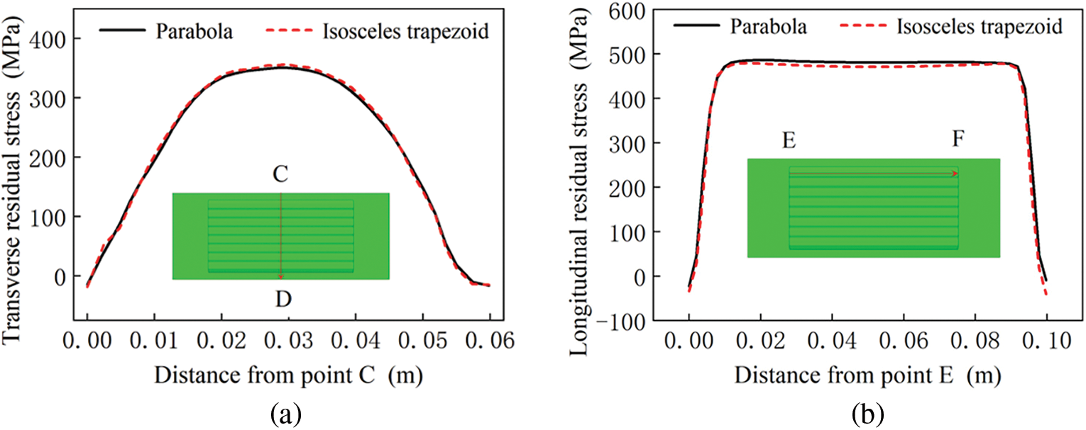
Figure 15: Comparison of residual stress between the two models (a) residual stress on the CD, (b) residual stress on the EF model
In addition, the calculation of the parabola-based FE model takes 580 min, while the trapezoid-based FE model takes 403 min. This means that the computation efficiency is improved by 30.5%, and the isosceles trapezoid-based model is computationally more effective than the parabolic-based model. Namely, the FE geometric modeling method based on the isosceles trapezoid proposed in this study has significant advantages in enhancing computational efficiency.
A geometric modeling method based on the isosceles trapezoidal curve for the multi-bead overlapping wire arc additive manufacturing deposition is proposed to replace the fitting curve based on the parabola modeling method. The effectiveness of the proposed modeling method based on the isosceles trapezoidal curve is verified by a variety of comparison methods.
1. The max average geometric deviation quotient of the isosceles trapezoid-based model is 7.5%. The geometric deviation and the error of the heat dissipation performance index of the overlapping model between the isosceles trapezoid-based model and the parabolic-based model are less than 7.5%, which means that the overlapping modeling method based on the isosceles trapezoid function has a high degree of geometric consistency and acceptable accuracy error than the parabolic-based model.
2. The thermal cycling curves, residual stress of different points of FE simulation and experiments, and residual stress distribution of FE simulation along the various paths indicate that the two models are highly consistent together and have high calculation precision. The isosceles trapezoid-based overlapping model can effectively replace the traditional parabolic-based model in the FE-coupled thermal analysis.
3. Compared with the fitting curve model, the computational efficiency of the finite element simulation of the isosceles trapezoid-based model is increased by 30.5% under the same calculation conditions. This means that the isosceles trapezoid-based model has significant advantages in computational modeling.
4. The proposed isosceles trapezoid-based modeling method can provide a reference and technical idea for high efficiency and high precision modeling of the finite element thermodynamics of the WAAM coupling simulation and other metal additive manufacturing technologies.
Acknowledgement: The authors are sincerely grateful to the anonymous referees and the editor for their time and effort in providing constructive and valuable comments and suggestions that have led to a substantial improvement in the paper.
Funding Statement: This research was funded by the National Natural Science Foundation of China (Grant No. 51705287) and the Scientific Research Foundation of Hubei Provincial Education Department (Grant No. D20211203).
Author Contributions: The authors confirm contribution to the paper as follows: Study conception and design: Xiangman Zhou, Jingping Qin, Seyed Reza Elmi Hosseini; data collection: Jingping Qin, Zichuan Fu, Min Wang; analysis and interpretation of results: Xiangman Zhou, Jingping Qin, Youlu Yuan; draft manuscript preparation: Zichuan Fu, Junjian Fu, Haiou Zhang. All authors reviewed the results and approved the final version of the manuscript.
Availability of Data and Materials: None.
Conflicts of Interest: The authors declare that they have no conflicts of interest to report regarding the present study.
References
1. Kawalkar, R., Dubey, H. K., Lokhande, S. P. (2022). Wire arc additive manufacturing: A brief review on advancements in addressing industrial challenges incurred with processing metallic alloys. Materials Today: Proceedings, 50, 1971–1978. [Google Scholar]
2. Vimal, K. E. K., Srinivas, M. N., Rajak, S. (2021). Wire arc additive manufacturing of aluminum alloys: A review. Materials Today: Proceedings, 41, 1139–1145. [Google Scholar]
3. Liu, J., Xu, Y., Ge, Y., Hou, Z., Chen, S. (2020). Wire and arc additive manufacturing of metal components: A review of recent research developments. The International Journal of Advanced Manufacturing Technology, 111, 149–198. [Google Scholar]
4. Le, V. T., Mai, D. S., Doan, T. K., Parisc, H. (2021). Wire and arc additive manufacturing of 308l stainless steel components: Optimization of processing parameters and material properties. Engineering Science and Technology, an International Journal, 24, 1015–1026. [Google Scholar]
5. Thapliyal, S. (2019). Challenges associated with the wire arc additive manufacturing (WAAM) of aluminum alloys. Materials Research Express, 6, 112006. [Google Scholar]
6. Derekar, K. S. (2018). A review of wire arc additive manufacturing and advances in wire arc additive manufacturing of aluminium. Materials Science and Technology, 34(8), 895–916. [Google Scholar]
7. Xia, C. Y., Pan, Z. X., Polden, J., Li, H. J., Xu, Y. L. et al. (2020). A review on wire arc additive manufacturing: Monitoring, control and a framework of automated system. Journal of Manufacturing Systems, 57, 31–45. [Google Scholar]
8. Liu, W. K., Li, S., Park, H. S. (2022). Eighty years of the finite element method: Birth, evolution, and future. Archives of Computational Methods in Engineering, 29(6), 4431–4453. [Google Scholar]
9. DebRoy, T., Wei, H. L., Zuback, J. S., Mukherjee, T., Elmer, J. W. et al. (2018). Additive manufacturing of metallic components—Process, structure and properties. Progress in Materials Science, 92, 112–224. [Google Scholar]
10. Cunningham, C. R., Flynn, J. M., Shokrani, A., Dhokia, V., Newman, S. T. (2018). Invited review article: Strategies and processes for high quality wire arc additive manufacturing. Additive Manufacturing, 22, 672–686. [Google Scholar]
11. Barath Kumar, M. D., Manikandan, M. (2022). Assessment of process, parameters, residual stress mitigation, post treatments and finite element analysis simulations of wire arc additive manufacturing technique. Metals and Materials International, 28, 54–111. [Google Scholar]
12. Zhao, H., Zhang, G., Yin, Z., Wu, L. (2011). A 3D dynamic analysis of thermal behavior during single-pass multi-layer weld-based rapid prototyping. Journal of Materials Processing Technology, 211(3), 488–495. [Google Scholar]
13. Huang, J., Guan, Z., Yu, S., Yu, X., Yuan, W. (2020). A 3D dynamic analysis of different depositing processes used in wire arc additive manufacturing. Materials Today Communications, 24, 101255. [Google Scholar]
14. Li, R., Wang, G., Zhao, X., Dai, F., Huang, C. (2021). Effect of path strategy on residual stress and distortion in laser and cold metal transfer hybrid additive manufacturing. Additive Manufacturing, 46, 102203. [Google Scholar]
15. Sun, J., Hensel, J., Köhler, M., Dilger, K. (2021). Residual stress in wire and arc additively manufactured aluminum components. Journal of Manufacturing Process, 65, 97–111. [Google Scholar]
16. Sun, L., Ren, X., He, J., Zhang, Z. (2021). Numerical investigation of a novel pattern for reducing residual stress in metal additive manufacturing. Journal of Materials Science & Technology, 67, 11–22. [Google Scholar]
17. Köhler, M., Sun, L., Hensel, J., Pallaspuro, S., Kömi, J. (2021). Comparative study of deposition patterns for DED-Arc additive manufacturing of Al-4046. Material & Design, 210, 110122. [Google Scholar]
18. Somashekara, M. A., Naveenkumar, M., Kumar, A., Viswanath, C., Simhambhatla, S. (2017). Investigations into effect of weld-deposition pattern on residual stress evolution for metallic additive manufacturing. International Journal of Advanced Manufacturing Technology, 90(5–8), 2009–2025. [Google Scholar]
19. Sun, L., Ren, X., He, J., Zhang, Z. (2021). A bead sequence-driven deposition pattern evaluation criterion for lowering residual stresses in additive manufacturing. Additive Manufacturing, 48, 102424. [Google Scholar]
20. Zhao, H., Zhang, G., Yin, Z., Wu, L. (2012). Three-dimensional finite element analysis of thermal stress in single-pass multi-layer weld-based rapid prototyping. Journal of Materials Processing Technology, 212(1), 276–285. [Google Scholar]
21. Ding, D. H., Pan, Z. X., Cuiuri, D., Li, H. J. (2015). A multi-bead overlapping model for robotic wire and arc additive manufacturing (WAAM). Robotics and Computer-Integrated Manufacturing, 31, 101–110. [Google Scholar]
22. Zhan, Y., Zhang, E., Fan, P., Pan, J., Liu, C. (2021). A novel finite element model for simulating residual stress in laser melting deposition. International Journal of Themophysics, 42, 56. [Google Scholar]
23. Nikam, S. H., Jain, N. K., Sawant, M. S. (2019). Optimization of parameters of micro-plasma transferred arc additive manufacturing process using real coded genetic algorithm. The International Journal of Advanced Manufacturing Technology, 106(3–4), 1239–1252. [Google Scholar]
24. Kik, T. (2020). Heat source models in numerical simulations of laser welding. Materials, 13, 2653. [Google Scholar] [PubMed]
25. Ghafouri, M., Ahn, J., Mourujärvi, J., Björk, T., Larkiola, J. (2020). Finite element simulation of welding distortions in ultra-high strength steel S960 MC including comprehensive thermal and solid-state phase transformation models. Engineering Structures, 219, 110804. [Google Scholar]
26. Ding, D. H., He, F. Y., Yuan, L., Pan, Z. X., Wang, L. et al. (2021). The first step towards intelligent wire arc additive manufacturing: An automatic bead modeling system using machine learning through industrial information integration. Journal of Industrial Information Integration, 23, 100218. [Google Scholar]
27. Obeid, O., Alfano, G., Bahai, H., Jouhara, H. (2018). Numerical simulation of thermal and residual stress fields induced by lined pipe welding. Thermal Science and Engineering Progress, 5, 1–14. [Google Scholar]
Cite This Article
 Copyright © 2024 The Author(s). Published by Tech Science Press.
This work is licensed under a Creative Commons Attribution 4.0 International License , which permits unrestricted use, distribution, and reproduction in any medium, provided the original work is properly cited.
 Downloads
 Citation Tools