An Optimal Node Localization in WSN Based on Siege Whale Optimization Algorithm

1  Introduction

A wireless sensor network (WSN) is constructed with various small devices called sensor nodes installed in an observing region for tracking some environmental or physical factors as a preeminent resource critical in multiple ramifications, including surveillance, military, healthcare, agriculture, and astronomy [1]. Because it possesses the advantageous characteristics of WSN [2], such as self-organization, speed, feasibility, and ease of implementation, it is frequently used across the Internet or cloud environment [3]. The tiny components of heterogeneous or homogeneous sensor nodes are presented in the WSN network to observe environmental and physical conditions [4]. As its name suggests, the sensor node can perceive, act upon, and transfer the information gathered from the source environment into the sink node [5] or base station using wireless communication [6]. The sensor node is built with various units like the location finding, transmitting, processing, power, and sensing modules [7]. Some sensor nodes have a global positioning system (GPS) in the location finding module [8], which helps to utilize these sensor nodes in various applications like deep water exploration, under liquid exploration, space exploration, hailstorm detection, fire detection, flood detection, even detection, surveillance application, environmental monitoring, and so on [9]. However, these nodes do not require any wired external infrastructure for communication like chemical clouds, and vehicles require mobile sensor nodes for gathering information from the external world via the Internet of Things (IoT) [10]. While designing the mobility-aided WSNs, the information on the coordinated position of a sensor node plays an essential role [11]. The location information is assumed as the data to be collected in some WSNs that randomly deploy the sensor nodes and distribute them at random locations [12].

Moreover, it is challenging to manually offer every node its unique position information. Therefore, for performing this process, other practical approaches require GPS, the principal location method primarily utilized for designing WSNs. It is impractical to attach every single node with a GPS device owing to financial cost and other factors comprising their size and incapability of working in various applications [13]. Localization methodology is one of the fundamental functions of WSN as an active research field that has recently resulted in designing multiple algorithms and models [14]. The two classifications of WSN localization techniques are range-free and range-based, which gauges distance during positioning [10,13]. Range-based positioning calculates the distance between the beacon node and the unknown node and has higher accuracy. Here, the term “beacon node” refers to a small sensor node that is aware of its coordinates and can be used to deploy other unidentified sensor nodes. In WSN deployment, unknown nodes do the locating task using the distance or network connectivity formula from the beacon nodes [10]. The range-free positioning performs better while being less expensive than the ranging-based positioning method because it does not check the requirements of applications, such as the higher precision need, and it has lesser localization accuracy [13]. When doing the placement, the range-free localization approach does not calculate the distance between the sensor nodes [8]. Since node localization is the main problem with WSN, it has problems finding the nodes to convey the data collected from the sensor nodes. It makes it difficult to estimate the information that the sensor gathers [15]. Therefore, this study investigates how to pinpoint a node’s location in a WSN precisely.

Additionally, one of the excellent dealing ways with the localization challenges problem is the meta-heuristic algorithms [16]. Various meta-heuristic approaches have been used in recent research on accuracy employing WSN node localization and developing numerous algorithms [17]. These methods are explicitly designed to deal with challenging optimization problems. There are several main categories of meta-heuristics algorithms, e.g., swarm-based, physics-based, and evolution-based techniques. Here, the Genetic algorithm (GA) [18] illustrates an evolution-based approach. Simulated annealing (SA) [19,20] is a typical example of a physics-based method. In contrast, several swarm-based techniques include Particle swarm optimization (PSO) [21], Whale optimization algorithm (WOA) [22], Harris hawk optimization (HHO) [23], Ant lion optimization (ALO) [24], Moth flame-fire optimization (MFO) [25], Gray wolf optimization (GWO) [26], and others.

The WOA is a recent swarm-based intelligent optimization algorithm that vividly simulates whales’ behavior of finding and attacking prey to model its mathematical formulas [22]. Compared with the meta-heuristic optimization algorithm, WOA has several distinct advantages, e.g., simple principle and understandable concept, few parameter settings, and strong optimization ability [27]. The algorithm has all existing benefits and disadvantages simultaneously; however, the WOA also has limitations of defects such as dropping into local optimum or slow convergence speed or/and low convergence accuracy when dealing with the complicated optimization problem. Thus, great academic significance is needed for the algorithm to give full play to the advantages and improve the known WOA shortcomings for a suitable solution to particular problems [28]. The WOA has also been recently enhanced with various strategies to prevent its disadvantages. For example, an adaptive whale optimization (AWOA) algorithm was suggested based on inputting the weight and bias matrix to increase the extreme learning machine’s performance robustness and accuracy [29]. An enhanced WOA (EWOA) was developed with its parameter of A and C were adapted as modifier and applied effectively to explore and exploit the search area to improve better performance [30]. The improved WOA (IWOA) was introduced approach based on combining the WOA exploitation and differential evolution exploration for global optimization solution [31]. A modified WOA (MWOA) was implemented to improve the nonlinear decreasing convergence factor to solve nonlinear problems better [32]. The no-free lunch principle theorem on optimization [33] states that no optimization approach best addresses every optimization problem. Unless we can make whatever prior assumptions about the optimization model we are trying to solve, no strategy can be expected to perform better than any other. More and more optimization methods would have been developed to suit specific problems thanks to the no-free lunch principle theorem [34].

This study also suggests an investigation strategy for enhancing WOA based on the siege mechanism, namely SWOA, for the complicated node localization problem in WSN. The method in the SWOA is figured out based on the siege mechanism, essential initial candidate locations, and inertia weighting parameters for avoiding the drawbacks of the local optimum and stagnation in the original one, which is referred to as escaping or allowing scoring goals in a difficult situation. Sieges enclose the target successfully applied in the Harris hawks optimization (HHO) [23] that incorporates information about running, grouping center, randomizing population division, and other related concepts or to jump out of the trap of falling the local optimum in the complex optimization problem solution. Harris eagles cooperate with other individuals in the eagle group during the foraging process. A soft and hard siege mechanism with fast convergence and population communication properties is established with the advantages of fast convergence speed and global optimization. The Harris eagle optimization algorithm takes this kind of cooperative behavior vividly expressed by mathematical formulas.

Siege’s enhanced whale optimization algorithm (SWOA) is a suggested strategy aiming to improve the performance solution to the challenging multimodals with more complex, e.g., one of those issues like localization in WSN and prevent the drawback of the trapping local optima additional algorithm. This section presents the proposed SWOA.

Several highlights are considered investigation of this study.

•   An exploration capacity is increased by hybridizing it with HHO’s siege mechanism to make the shrinkage and encirclement whale mechanism robust and adaptable to the specific node localization problem.

•   A re-initialization of essential initial candidate locations employs inertia weighting parameters. It makes the closer expecting solution and avoids the local optimum’s drawbacks to increasing population variety.

•   The node localization model is figured out for the objective function with Err as the formulated functional derivation, del as a specifying delay, Eng as deriving the energy function, and the path loss is denoted as PL, and received signal strength.

•   The outcomes demonstrate that the suggested algorithms can significantly raise SWOA’s performance.

The remaining parts of the study include the following sections. Section 2 presents a literature review with the node localization problem statement and standard model definitions, and reviews the original WOA approach. Section 3 introduces the application siege mechanism to enhance the WOA algorithm (SWOA), implement tests to verify the performance in comparison, and analyze the results. Section 4 presents the SWOA for optimal WSN Node Localization. Finally, Section 5 draws a summary as the conclusion.

2  Literature Review

This section presents a statement of the node localization in the WSN problem and reviews the node localization situation developments and the original WOA algorithm.

2.1 Node Localization Problem Statement

The sensor nodes in a WSN gather information like humidity, temperature, and pressure dependent on the specific region [35]. The node localization strategy, which is widely used in many industries due to cheaper sensor nodes, is the WSN trend-setter issue. Localization of sensor nodes needs to be done accurately when considering the WSN to enhance the network’s performance in various real applications, e.g., monitoring, military, healthcare, agriculture, and astronomy applications [36]. However, it is very challenging to determine the accurate location of the mobile sensor nodes because of their time-variant movement. Therefore, various metaheuristic and profound studies algorithms are developed for performing node localization in WSN. Table 1 lists some of these works with a short brief description of features and challenges.

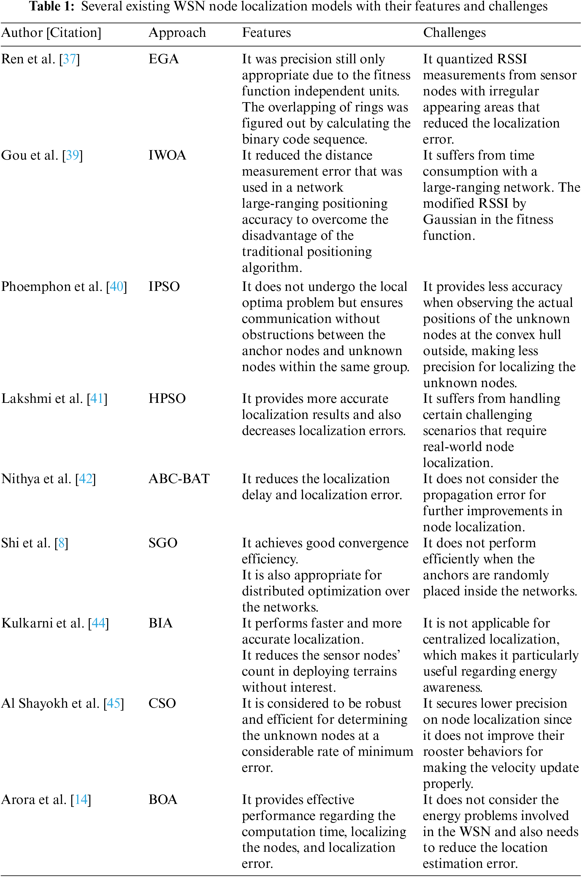
The elitist genetic algorithm (EGA) [37] adopted a preservation strategy for optimal node localization with an RSSI quantization based on sensing disks of nodes. The whale optimization algorithm (WOA) [38] and improved whale optimization algorithm (IWOA) [39] for the node location in WSN. The distance measurement error was reduced with the modified RSSI by Gaussian that was used in a network large-ranging positioning accuracy to overcome the disadvantage of the traditional positioning algorithm.

The improved particle swarm optimization (IPSO) [40] used a hybridized node localization model with improved particle swarm optimization into the local optima problem and ensured communication without obstructions between the anchor nodes and unknown nodes within the same group. However, it could provide more accuracy when observing the actual positions of the unknown nodes at the convex hull outside that, which makes less precision for localizing the unknown nodes. Hybrid Particle Swarm Optimization (HPSO) [41] provided more accurate localization results and decrease localization errors. But, it suffers from handling challenging scenarios requiring real-world node localization. ABC-BAT [42] reduced the localization delay and localization error. Yet, it did not consider the propagation error for further improvements in node localization.

Krill Herd Optimization Algorithm (KHA) [43] reduced the error rate regarding the mean absolute error and root means square error, propagation error, and localization error. But, it depends on the length of the communication radius to increase the success rate of localization. Sequential Greedy Optimization Algorithm (SGO) [8] achieved good convergence efficiency and is also appropriate for distributed network optimization. Yet, it only performs efficiently when the anchors are randomly placed inside the networks. Bio-inspired Algorithms (BIA) [44] performed faster and more accurate localization and reduced the sensor node count in deploying terrains without interest. On the other hand, it is not applicable for centralized localization, which makes it particularly useful regarding energy awareness.

Chicken Swarm Optimization (CSO) [45] is considered robust and efficient for determining the unknown nodes at a considerable rate of minimum error. However, it secures lower precision on node localization since it needed to improve their rooster behaviors for making the velocity update properly. Butterfly Optimization Algorithm (BOA) [14] provided effective performance regarding the computation time, localizing the nodes, and localization error. On the other hand, it does not consider the energy problems involved in the WSN and needs to reduce the location estimation error. These challenges in the existing localization scheme in WSN motivate the development of a new heuristic strategy for localizing the unknown nodes in WSN.

As is noted, a good monitoring and tracking application relies heavily on location accuracy. The existing works suffered from handling specific difficult conditions that need real-world node localization, tried to make it more accurate for localizing the unknown nodes, and did not consider propagation error for further advancements in node localization. The scheme positioning system’s executed time consumption should be considered when there is a large-scale ranging network. It benefited energy awareness because it did not require centralized localization and functioned well when the anchors were dispersed throughout the networks. Additionally, they neglected to consider the WSN’s energy-related issues and the need to lower location estimation errors. Creating a new metaheuristic technique or improving the existing algorithm for suitable localizing the unknown nodes in WSN is motivated in this study by these issues with the current localization scheme in WSN.

2.2 Node Localization in WSN

The problem definition of node localization in WSN possesses many sensor nodes, such as anchors or beacon nodes, unknown nodes or dumb nodes, and settled nodes, where every node has a communication range [36]. An anchor node is depicted as a small node that knows its own position with coordinates in the network. Unknown node is depicted as nodes unaware of their location in the network; later on, they can be identified, also termed free nodes, by deploying localization algorithms [15,46]. A settled node is initially also a dumb node; afterward, it can somehow manage to determine the position by localization scheme. To successfully carry out monitoring or tracking applications, which is a process of selecting or estimating a location known as localization, the position must be aware of sensor nodes. As a result, in the WSN setting, location finding presents a significant issue. Either the range stage or the estimating phases are included in the process. With the use of angle of arrival, RSSI, Time of arrival, the former, or distances, are measured between the nodes [47]. The estimation stage is then completed by considering the range value and minimizing the localization error.

Fig. 1 depicts a typical calculation in node localization issues in WSN via anchor nodes to the unknown node. It is an expected WSN localization issue with dashed and solid arrows, respectively, and indicates anchor-to-anchor and anchor-to-unknown node measures. The WSN deployment area are divided into grid cells with the node’s communication radius. The adjacent grid cells must guarantee direct communication between two nodes. In order to determine which cell the node would belong to, it is assumed that it knows the location coordination of its neighbor.

Figure 1: A typical calculation in node localization issue in WSN via anchor nodes to the unknown node

Let us assume the WSN is a symmetric type, illustrated as a Euclidean graph E=(A,B). Here, we could assign the vertices A as a set as A={a1,a2,…,az} and B indicates the edges as B={b1,b2,…bm} where b is set to coordinates (x, y). Subsequently, the communication is happened by computing the distance between the two nodes. Hence, the two nodes as ax and ay, and their estimated distance is dx,y≤m, in which m gives the maximum distance among the nodes. The communication is done only when the distance becomes less than the variable as m. Given E=(A,B) of WSN, a set of anchor nodes with its known position coordinates as (xi,yi) for all i∈I, where I is a number of anchor nodes (max is M). Further, it aids in estimating the location or position of unknown nodes coordinated as (xj,yj) for all j∈J, where J a number of unknown nodes (max is N). Thus, influencing the localization algorithm on the unknown node makes it a settled node by identifying the position as S solution.

The objective function is mainly designed with the fitness approaching value to validate the efficacy of the node localization approach in WSN. Once the optimal location is determined, it aids in reducing the error factor in locating the sensor nodes. Here, the localization error is mainly calculated by the distance estimation concerning anchor nodes and sensing ranges of the chosen dumb node and the beacon node. The mathematical expression of the objective function is given formula as follows:

ObF=argminSz∗[Err](1)

where Sz∗ is a resultant optimal position as a solution; Err denotes the error measure that is determined by using the following formula:

Err=del+1Eng+1RSS+PL(2)

Here, Err is the formulated functional derivation, del specifies the delay, Eng derives the energy function, and the path loss is denoted as PL, and RSS (Received signal strength) is “the intensity of the acquired signal by the wireless access point”. These factors are all closely related to the distance of the coordinates of the anchor and target nodes. The distance between the anchor nodes within the sensing range of the target node ưith the coordinate known as position (x,y) is used to identify the target node.

2.3 Basic WOA Algorithm

The WOA simulates the whale’s predation action. It divides the whale’s predation process into three steps according to the whale’s predation characteristics, that is, three position update methods: shrinkage and encirclement, spiral position update, and random search [10].

Shrink and surround is a phase of the place whales can perceive the area where the prey cover it and is located for the position of the optimal design in the hunting or search space is inconsistent with the previous position. The WOA optimization algorithm assumes that solution S(t)={s1,s2,…,sN} is the current candidate solution, with N as the population number, t is the current generation of iteration and the best candidate solution S∗ is the target prey or close to the optimal solution. In this phase case, the whale defines the best search agent with S∗; other search agents S will then try to change positions and move closer to the best search agent. The following formula describes the hunting behavior of shrinking surroundings:

S(t+1)=S∗(t)−α.D1,D1=|β.S∗(t)−S(t)|,(3)

In the formula, t represents the current number of iterations, α, and β are vector coefficients, S(t) is the current position, S(t+1) is the next position, D1 is the absolute value of the difference between β times the prey position and the current whale position, S∗(t) is the position vector that currently obtains the optimal solution. If there is a better solution in the result of each iteration, that is, the fitness value of the position at this time is less than the fitness value of S∗(t), then the whale position vector is set to the new S∗(t). The formulas for calculating α and β are set as follows:

α=2.a.r1−a,β=2.r2,(4)

where r1 and r2 are random numbers within [0, 1], a is set to 2−2tTmax, with Tmax is the maximum number of iterations, β is set in the value range of a is [0, 2], and it changes linearly with the increase of t.

Updating whale location phase is figured out with two ways to update the whale’s position: a spiral position update and a random search. The whale’s position update method at a particular time ensures that the whale has an equal probability of choosing a spiral position update or random search at the same time. A random number p is used to switch the updating ways with random in the range of [0, 1]. The value of p randomly selects the update method of the whale position.

Spiral position update is carried out when p ≥ 0.5; the spiral position update method is selected, and the spiral position update equation is established by simulating the way the whale spirals around the prey, which is used to update the next whale’s position. The calculation formula is given as follows:

S(t+1)=D2.ebl.cos(2πl)+S∗(t),D2=|S∗(t)−S(t)|,(5)

where D2 represents the distance between the prey and the whale, b is a parameter that controls the shape of the spiral (b is set to 1 in the experiment), and l is given as the following formula:

l=(a1−1)∗r3+1(6)

where, a1 is a parameter that changes linearly in [−2, −1], and it is set to (−1−tTmax), it means the value range of l is [−2, 1], and r3 is a random number between [0, 1].

Random search update is carried out when p<0.5, and the random search position update formula is selected. The random search is divided into two ways. When |α| < 1, the whale is moving toward the prey. Eq. (4) to surround the target. When |α| ≥ 1, the whale moves beyond the position where the prey exists. At this time, the whale will give up the previous moving direction and randomly search for a new update position in other approaches to prevent falling into the local extremum.

A randomly selected whale position is formulated given the following equation:

Drand=|β.Srand(t)−S(t)|S(t+1)=Srand(t)−α.Drand,(7)

where Srand(t) and Drand represent a randomly selected whale position vector and the absolute value of β times the difference between Srand(t) and S(t), respectively, α and β are mentioned above.

Several variants of the WOA have been developed recently that, includes the AWOA [29] suggested an adaptive one by inputting the weight and bias matrix to increase the optimal learning machine’s performance, EWOA [30] developed by adapting parameters of A and C as modifiers and applied effectively to explore and exploit the search to improve better performance, IWOA [31] introduced by combining the WOA exploitation and differential evolution exploration for global optimization solution, and MWOA [32] implemented by modifying the nonlinear decreasing convergence factor to solve nonlinear problems better. Unlike the existing variants, we consider initial candidate locations, inertia weighting, and balancing the global and local search for both adapting parameter and targeting problems. The other motivation is based on the no-free lunch [33] principle theorem on optimization states that no optimization approach best addresses every optimization problem.

3  Siege’s Enhanced Whale Optimization Algorithm (SWOA)

Siege’s enhanced whale optimization algorithm (SWOA) is a suggested strategy aiming to improve the performance solution to the challenging multimodals with more complex, e.g., one of those issues like localization in WSN and prevent the drawback of the trapping local optima additional algorithm. This section presents the proposed SWOA based on the siege mechanism, essential initial candidate locations, and inertia weighting parameters for avoiding the drawbacks of the local optimum and stagnation in the WOA.

3.1 An Enhanced Whale Optimization Algorithm

The whale position update process randomly selects the position update mechanisms, so the practical updating whale locations cannot be specified by changing the role of the leader S∗(t) leads to the problem that the convergence process ends prematurely. That is, when solving the optimization complex problem, it may quickly drop to the local optimum, and finally, the quality of the solution of the optimization algorithm decreases. An enhanced whale optimization algorithm is proposed based on the siege mechanism for the existing problems in the traditional whale optimization algorithm.

The harris eagle siege mechanism is applied to speed up the whale hunting; add an inertia weighting parameter at the end of each whale hunting iteration. The initial population location of the random generation algorithm is mapped by the chaotic Tent method so that the population is distributed more uniformly and the convergence speed of the algorithm would be accelerated; a new nonlinear parameter a is proposed so that the whale optimization algorithm can adapt to complex nonlinear problems; the fitness control is introduced mechanism, by controlling the update of the population position, to prevent the update from stagnation, and to improve the ability of the algorithm to jump out of the local optimum. The flowchart of the SWOA is shown in Fig. 1.

Re-initial whale’s population location: As whales can perceive the area where the prey is located and surrounded, the position of the optimal design in the searching or hunting space is inconsistent with the previous position in solving the function optimization problem. The initial population location has a critical role in ensuring the population’s diversity, leading to faster optimization performance of the algorithm [48,49]. The whale algorithm usually uses randomly generated data as, on the one hand, the chaotic map has randomness and regularity.

On the other hand, for the intelligent optimization algorithm based on population iteration, the initial population’s quality affects the algorithm’s solution accuracy and convergence speed. It assumes that the current best candidate solution is the target prey or close to the optimal solution whale defines the best search agent; other search agents will then try to change positions and move closer to the best search agent.

The following formula describes the characteristics of the chaotic map that can make the algorithm effectively escape from the local optimum, thereby maintaining the diversity of the population and improving the global search ability. The Tent map is used to initialize the whale candidate location, and the reference [49] takes u=0.7; its limit parameter expression is as follows:

g(i+1)={g(i)0.70≤g(i)<0.7,1−g(i)0.30.7≤g(i)≤1,(8)

Here g is a generating variable for initialization given randomly (0, 1) over iteration for generating chaotic sequence {g1,g2,…,gn}, i=0,1,…,n−1. For the initialization, agents can be applied with the Tent map for the sequence following the solution.

St=St,min+(St,max−St,min)gt(9)

Here, St,min and St,max represent the lower and upper boundaries of the S space search with its dimension.

An inertia-weight is a parameter that is used to adjust controlling the momentum of agents’ contribution in previous generation search moving forward. It can be seen that the size of the inertia weight value would affect the ability to exploit and explore search phases.

Let w be an inertia weight coefficient that is added to SWOA in the optimizing process. Its expression of the updating location is figured out as follows:

S(t+1)=w⋅S∗(t)+D2.ebl.cos(2πl)(10)

Here, w is a parameter of inertia weight that would be increased gradually from [½ to 1] over the iteration. The coefficient of inertia weight is given as follows:

w=12×tTmax+12(11)

Here t and Tmax are the current and Max iteration numbers.

Harris hawk optimization siege mechanism: Siege is an escape mechanism or allowing scoring goals in a difficult situation in battle [23]. A siege is launched when an aggressor runs into an area or stronghold that cannot be quickly captured and will not give up. Sieges entail enclosing the target to prevent the delivery of supplies and the reinforcement or ejection of warrior fighters.

This siege mechanism has been successfully applied in the HHO to jump out of the trap of failing the local optimum in the complex optimization problem solution. The HHO simulates the predation action of the Harris eagle and simulates its action with mathematical formulas.

The algorithm vividly simulates the Harris eagle’s Siege and predation mechanism, which gives the algorithm a robust global search ability. In the WOA, finding the optimal position is often the random exploration of a single whale individual. The lack of communication between individuals and groups makes some individuals far from the prey to conduct many useless investigations.

The siege strategy in the HHO would be used to improve the position of the WOA to a certain extent. The formula of the HHO is applied to adapt for the WOA exploring phase updating equation as follows:

S(t+1)={Y, f(Y)<f(S(t))Z, f(Z)<f(S(t))Y=w⋅S∗(t)−γ⋅D1Z=w⋅S∗(t)−α⋅D1+τ⋅LF(M),(12)

In the formula: f(S(t)) is the position fitness value of S(t), which means that a particular position is substituted into the fitness function to calculate its fitness value; γ is an M-dimensional random vector on the uniform distribution of (1,M); LF(M) is Levi’s flight formula with the M-dimensional random vector generated by Levi’s flight, that is given as follows:

LF(M)=0.01×u×(Γ(1+θ)×sin⁡(πθ2)Γ(1+θ2)×θ×2θ−12)1β|v|1θ(13)

Here, Γ(x) is a Gamma function, u and v are random values between (0, 1), and β is set to 1.5.

The exploring phase capability is the key for the group to use the position update method to explore a wide search area and avoid the algorithm falling into the local optimum. However, the exploiting phase capability is mainly to use the existing information of the group to analyze the solution space. The local search is carried out in some neighborhoods of the algorithm, which has a decisive influence on the convergence speed of the algorithm. The convergence factor with a significant change has a better global search ability and prevents the algorithm from falling into a local optimum; a smaller convergence factor with a more vital local search ability can speed up the convergence speed of the algorithm [13]. However, the convergence factor a in the whale optimization algorithm decreases linearly from 2 to 0 with the number of iterations, which must fully reflect the exploration and exploitation process optimization. The parameter a is directly controlled by modifying the coefficient adapted to its a from Eq. (4), and the change of coefficient a leads to specific changes in the random search and shrinkage encirclement mechanisms.

a=2.(1−tTmax),(14)

Here, Tmax is the maximum number of iterations, and t is the current number of iterations. A nonlinear decreasing convergence factor with rapid change in the early stage and relatively slow change in the later stage is designed to balance the exploration and exploration. When the algorithm keeps exploring and exploiting the search position during the iterative process, the optimal position frequently needs to change the fitness value of the whale’s position after the iterative update continues. The spiral position update formula is to update the current situation; otherwise, the following position update formula is judged according to | α | as a flowchart, as shown in Fig. 2. Algorithm 1 illustrates a siege’s enhanced whale optimization as its pseudo-code SWOA.

Figure 2: A flowchart of the pseudo-code SWOA algorithm

3.2 Experimental Results with Benchmark

This subsection analyzes the qualified performance of the suggested SWOA algorithm by comparing it with the selected popular algorithms. A popular suit test with benchmark functions of the CEC2013 consists of 23 tasks (F1~F23) with variable-dimensional parts used to test and evaluate the SWOA algorithm. Three sets of comparison-experimental tests consist of with the original optimization algorithms, with different optimization algorithms, and with improved WOA algorithms for the selected benchmark functions of the CEC2013 test suit. The practical testing compared to the original optimization methods includes the WOA and HHO [23] algorithms.

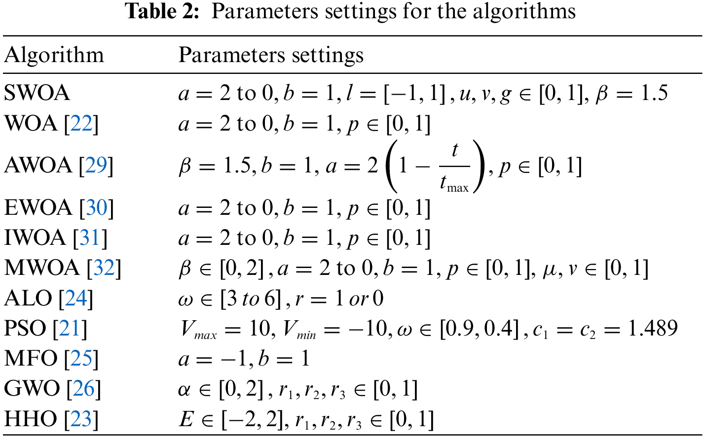
The experimental test with other optimization algorithms consists of the ALO [24], GWO, MFO [25], and PSO [21] algorithms. The practical test with different improved whale optimization algorithms has the AWOA [29], EWOA [30], IWOA [31], and MWOA [32]. Various complexity types and dimensions settings in the selected functions in test suites are used, such as unimodal (F1~F3), multimodal (F4~F19), hybrid (F10~F16), and compound (F17~F23) test functions. The obtained results of the algorithms for the test are the global optimum presenting in the form of tables and figures.

Table 2 lists the parameter settings for the algorithms. It is a fair comparison and done in the same condition setting of the number of iterations, Tmax is set to 1000, population size is set to 80, and all optimization algorithms are run independently 30 times to avoid randomness and ensure the accuracy of the experiment.

The first test set of comparison with the original optimization algorithms is implemented by uniformly setting the same population size, number of iterations, and dimension, e.g., 30, 50, and 100D. The results of the SWOA algorithm are compared with WOA [22] and HHO [23] and verified by experiments. Table A1 shows the calculation results of the average and standard deviation of the optimal values of the original algorithms in different dimensions over run separately 30 times. For each pair in Table A1, the average and standard deviation of the optimal values of proposed result values compared with the original algorithms are summarized in the last column. The summarized column uses symbols such as ‘+/−/=,’ which means better, worse, and equivalent. It is seen that the number of wins belongs to the SWOA algorithm. Fig. A1 shows the three original optimizations algorithm, the convergence curves of F1, F3, F5, and F6 in the same dimension of 50D, where the horizontal axis is the number of iterations, and the vertical axis is the optimal fitness value. It can be seen from the figure that in different dimensions, the optimization convergence characteristics of the algorithm have not changed significantly, the SWOA algorithm is only slightly lower than the HHO algorithm on the F1 and F6 test function, and the SWOA algorithm shows excellent convergence accuracy and speed on F3, and F5. The compared results prove that the SWOA is better than the original WOA and HHO.

The second test set is implemented experiment and comparison with different optimization algorithms. Several popular developed optimization algorithms in recent years are selected, e.g., ALO, GWO, MFO, and PSO algorithms for the test benchmark functions. Table A2 shows the calculation and comparison of the optimal fitness value of different optimization algorithms under the same dimension, running 30 times separately. The optimal result values are statistical mean and standard deviation (std.) calculated by the various algorithms for the functions with dimensional of 30D and 100D. The comparison summary of the experimental data is put in the last table with a paired comparison with the SWOA. The symbols >/~/< are better, equal, and worse. The statistical result shows that the SWOA has more ‘better’s numbers than the others, which means the SWAO provides excellent performance.

The third test set is implemented experiment and comparison with variant improvement strategies for the WOA algorithm. Several developed improved WOAS algorithms are selected, e.g., AWOA, EWOA, IWOA, and MWOA algorithms, for the test functions with the same condition settings, population size, iteration, and the number of run times. Table A3 compares the optimal results of different improved WOA algorithms, e.g., AWOA, EWOA, IWOA, and MWOA, with the SWOA approaches. It displays the calculation and comparison of the optimal fitness value of variant improved WOA strategies for the test functions in the same dimension, running 30 times separately. The optimal result values are statistical mean and std calculated by the various algorithms for the functions with dimensional of 30D and 100D. The last table summarizes the comparison of the experimental data with a paired comparison with the SWOA with >/~/< of symbols that are better, equal, and worse. The statistical result shows that the SWOA has more ‘better’s numbers than the others, which means the SWAO provides excellent performance.

Fig. A2 contains the convergence curves of the different optimization algorithms and the SWOA for selected functions of F1, F3, F4, F5, F6, F7, F11, and F13 in the dimension of 100D. Comparing the convergence curves of the algorithms, it can be seen that in the different modal benchmark tests in 100-dimensional, the SWOA has a better convergence speed of optimal fitness values. There are significant differences between the algorithms; through the sign test, it can be seen that the quality of the SWOA solution in different tests is better than the above-selected algorithms. The above experimental data shows that the SWOA has excellent optimization performance.

4  SWOA for Optimization WSN Node Localization

Stepwise presenting subsections are described as following stepwise execution in designing an optimal node localization with the SWOA strategy in WSN. The objective function frame as the efficient localization scheme in WSN would be stated via solving the objective functional derivation regarding factors like delay, path loss, energy, and RSS for optimizing the anchor nodes to reach the target nodes in sensor field simulation. A node localization schematic in optimizing node positions for anchor nodes towards the target nodes using the newly recommended SWOA algorithm. Update the objective function in optimizing using t the optimal solutions candidates of the SWOA for reaching the higher convergence rate and getting the location of anchor nodes based on the anchor nodes. The results implement simulation with scenarios of different WSN networks, e.g., network area, number of target nodes, anchor nodes, and sensing range, to perform the node localization process. The best localization solution in WSN in terms of location coordinates of anchor nodes is found for the solution with minimum fitness. The resolution is the optimal solution that reaches higher localization performance with a better convergence rate.

4.1 Modeling Objective Function Frame

The node localization strategy to reach the target nodes in the sensor field using a new SWOA algorithm for minimizing localization errors with the optimized anchor node provided a limited resource of the solution element. As a result of resolving the objective functional derivation concerning variables, including latency, path loss, energy, and RSS, are recognized as the effective localization strategy in WSN. The designed node localization model for WSN is derived in the following manner with the objective function ObF is referred to in Eq. (1) that mainly designed with the fitness approaching value to validate the efficacy of the suggested node localization approach over WSN as follows:

ObF= argmin{ANj}(1Eng+1RSS+PL+del)(15)

Here, Eng derives the energy function, del specifies the delay, and the path loss is denoted as PL, and RSS is “the intensity of the acquired signal by the wireless access point”.

The energy function of anchor nodes is estimated as derived as follows:

Eng=(dis2⋅ρ⋅Fsl+(TXeng+ADeng)⋅ρ),(16)

Here, Fsl and ρ are coefficients loss for free space derived of anchor nodes; TXeng and ADeng are the transmission energy and the acquired energy, respectively.

The node localization strategy to reach the target nodes in the sensor field using a new SWOA algorithm for minimizing localization errors with the optimized anchor node where provided limited resources of the solution element. Once the optimal position is determined, it aids in reducing the error factors related to the distance estimation via energy Eng in locating the sensor nodes. Hence, the position optimization is taken place by the SWOA algorithm. Here, the localization error is mainly calculated by the distance estimation concerning anchor nodes and sensing ranges of the chosen dumb node and the beacon node in WSN. Euclidean distance has specified the coordinate known as positions used to identify the target node (rtj,stj), and the location of the anchor node is referred to as (rj−sj).

disj=(rtj−rj)2+(stj−sj)2(17)

Here, disj is the distance between the anchor nodes and target nodes. The recommended node localization strategy gets the node information via the position of anchor nodes in the direction of the optimal target nodes or unknown nodes by applying the SWOA algorithm, where the nearest target nodes are reached by minimizing node localization errors. The anchor nodes are specified as ANj, the number of anchor nodes is considered as O, and j=1,2,…,O and the target nodes are represented as TNt, where t=1,2,…,T, the in which a number of target nodes T.

The derivation concerning the variable of the RSS is given as follows:

RSS=RPNP(18)

Here, the term NP specifies the noise power, and RP illustrates the receiving power that describes the RSS of anchor nodes; that is, in the experimental setting, it is set to −91 to −35 dBm. The path loss PL variable is modeled by formulating the normal log for defining the communication range of nodes.

PL=LN(Rangec)(19)

Here, Rangec is the communication range of a node, in which the pass loss exponent is used for determination and setting a Rangec=10(pwtr−pwτ10μ), where the path loss factor is denoted as μ, Pwτ derives the least threshold receiver power attained by nodes, and the transmitted power is derived as Pwtr. In the experimental section, it is set to 10 to 30 m. Localization delay is known as de, which is defined as the time variation while broadcasting a request message by a sensor node and when it achieves its place as formulated in Eq. (20).

del=RMtime−LNtime(20)

Here, LNtime, and RMtime are the time while the position coordinates are achieved for a node and the time while a request message is broadcast, respectively. The best localization solution in WSN in terms of location coordinates of anchor nodes is found via optimizing objective functional derivation for minimum fitness solution for expecting taken as the optimal solutions that reach higher localization performance with better convergence rate.

4.2 Node Localization Schematic in WSN

As mentioned, the sensor nodes in WSN are employed to gather the details, e.g., humidity, temperature, and pressure, which rely on the corresponding location to be collected with concern WSN for the node localization scheme owing to less-cost sensor nodes. The WSN deployment region must be divided into several virtual grid cells based on the node’s coordination and communication radius. The adjacent grid cells must guarantee direct communication between two nodes. In order to determine which cell the node would belong to, it is assumed that it knows the location coordination of its neighbor. For instance, a specific area has three subrings intersecting with r as a grid unit length, which means that the mesh is surrounded by three rings covered; multiple rings cover the actual location of the grid as equal to 3r; as a result, the more covered grids there are, the more likely it is that there will be unknown nodes in the area. The fundamental idea behind building an ideal model is establishing a boundary condition for the optimization algorithm constraint that must be specified to control the forward updated solution. It ensures that any two nodes in adjacent cells can interact with each other directly, removing the need for noise-reducing device terminals and ensuring that cell radius requirements are met as (3r)2τi+(3r)2τi+1≤R2. The formula can be drawn from the expression rewritten as follows:

r≤R32,(21)

where R is the communication radius; a set to grid unit length is met a condition Eq. (21); τi is an effective noise coefficient to node i, generally set to 1.

Considering these constraints, the metaheuristic optimization algorithms, e.g., bio-inspired algorithms, swarm intelligence, and genetic-based heuristic approach, are applied for node localization and formulated the equations for reducing the localization error among the nodes in WSN. Over the iteration, the algorithm is deployed to find the position of unknown nodes that continues till the dumb nodes become settled nodes. Fig. 3 illustrates a typical scheme of a heuristic algorithm for node localization in WSN using the SWOA strategy. The node localization strategy with the SWOA algorithm in WSN is optimized over the system node localization model.

Figure 3: Schematic representation of optimal node localization issue with minimizing error localization in WSN based on the SWOA approach

The prime intent of the suggested model is to resolve the node localization issue over the WSN sector and build the objective function of node localization based on the SWOA with distance computation and localization error. The distance measurement and range value among the nodes, the novel method can mitigate the localization error. Due to the attainment of fewer errors, the proposed procedure ensures effective localization performance. The simulation results are validated and compared against other existing heuristic optimizations, which is reviewed in the following subsection.

4.3 Results and Discussion

The obtained results of the node localization framework in WSN and simulation setup from the proposed SWOA are analyzed to evaluate performance. Based on convergence analysis and statistical analysis, the performance of the suggested model is compared with several previous schemes in the literature with model condiction. Here, the total iteration count is set at 1000, the number of populations is taken to be 40, and the number of dimensions is set to the number of anchors and unknown sensor nodes, along with the node’s (x, y) coordinates.

Fig. 4 compares the obtained convergence by SWOA with the original WOA [38] for the objective function as designed fitness localization with 30/60 anchor/target nodes for two cases in areas 60 × 60 and 100 × 100 m2, respectively. It can be seen that the SWOA produces convergence faster than the WOA in the same condition simulation settings.

Figure 4: Comparison of the obtained convergence by the SWOA with the original WOA for fitness localization with 30/60 anchor/unknown nodes: (a) cases in areas 60 × 60 m2, (b) 100 × 100 m2, respectively

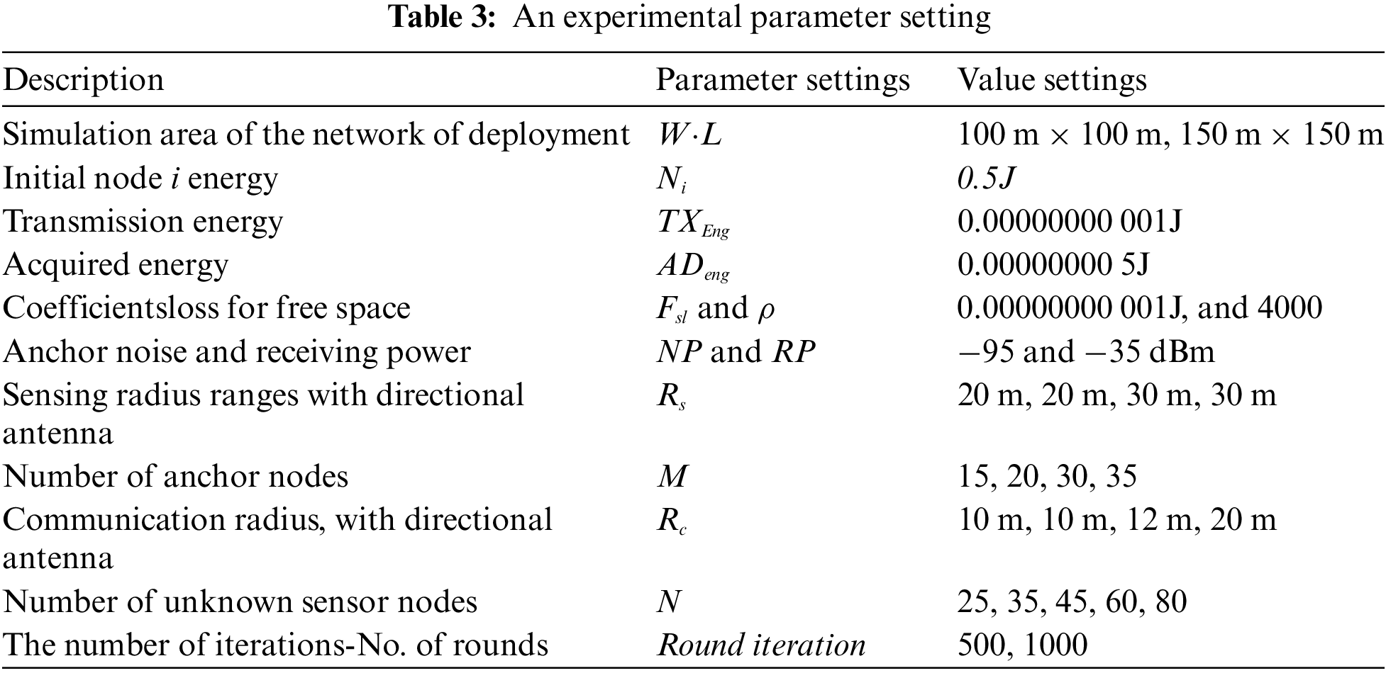
Moreover, the obtained results of the suggested SWOA method are compared with the previous scheme algorithms, including EGA [37], IPSO [40], KHA [43], CSO [45], and IWOA [39] algorithms. Experimental parameter settings are initialized for the scheme simulating in the compared fair of the algorithm of the WSN for node localization.

Table 3 lists considered parameter settings simulating schemes. The directional antenna is used for the WSN localization approach, which is range free with four directional antennas connected with nodes. The sensor nodes and the coordinates that detect the beacon messages are determined using a simple processing approach that evades the sensor node communication effects of changes in the range of transmission of the WSN nodes.

In most operations during the routing process, it becomes necessary to gather neighbor information to understand the nodes’ state, convey nodes’ parameters (energy, memory, and nodes’ id), and so forth, using probe messages. The protocol is used in networks to send beacon and probe messages by taking the control packet with piggybacking for updating the neighbor node about node status or querying some neighbor nodes. Additionally, communication networks commonly use broadcast, unicast, multicast, or any cast. Broadcasting or beacon messages are discouraged unless necessary because of the “always broadcast nature” of messaging in wireless communication.

Table 4 compares results obtained from the proposed SWOA with the other methods: the IPSO, KHA, SGO, SCO, and BOA algorithms, in situations of rate percentage of coverage, executing times, round iterations to convergence reaching, and sensor nodes for monitoring region sizes.

The performance of the routing protocol is also impacted by and dependent on the deployment of WSN applications. Because the sensor nodes are dispersed at random, an ad hoc infrastructure is produced. To enable connection and energy-efficient network operation, optimum clustering is required if the resulting node distribution is not uniform. Inter-sensor communication typically takes place within small transmission ranges due to energy and bandwidth restrictions.

As a result, it is very possible that a route will have several wireless hops. In this work, Span [50] is chosen as some nodes as coordinators based on their placements since it is the energy-efficient coordination mechanism for topology maintenance in ad hoc WSN. In the distributed, randomized method Span, nodes locally decide whether to go to sleep or to become a coordinator in a forwarding backbone. Each node bases its choice on an estimation of the number of neighbors that will profit from its being awake and the energy supply.

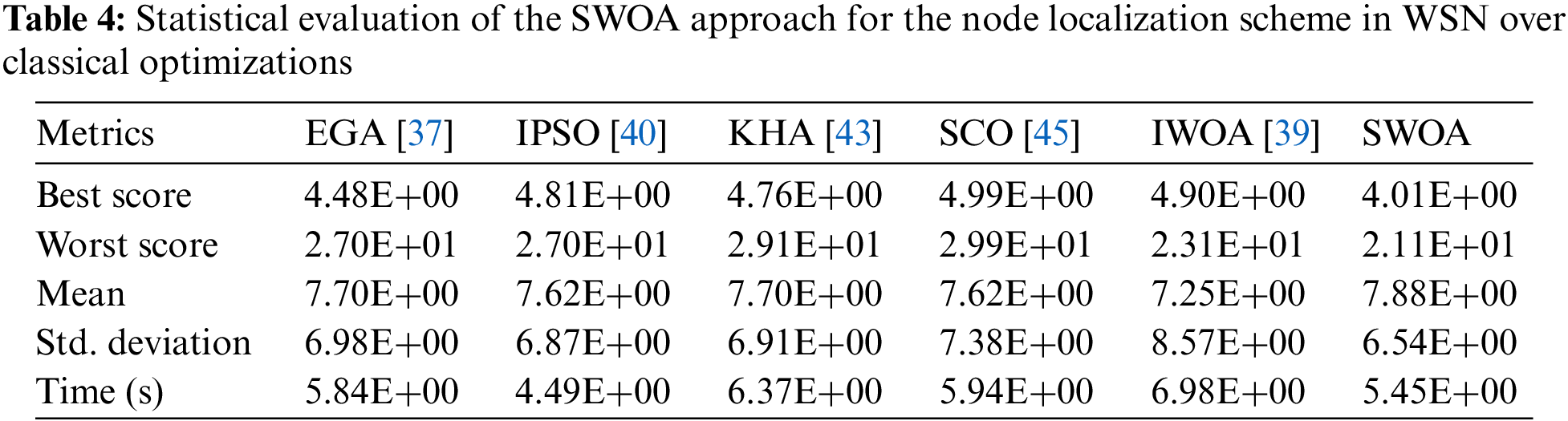
Several metrics over iterations represent analysis for the node localization scheme based on the SWOA with the objective function, e.g., the best, worst, mean, standard deviation score values, and computation time of different optimization approaches. A statistical evaluation of the proposed SWOA for the node localization scheme in WSN over classical optimizations. The SWOA algorithm attains better quality performance in contrast with conventional algorithms such as EGA, IPSO, KHA, CSO, and IWOA approaches.

Fig. 5 shows the optimal graphical demonstration of the SWOA for some node localization under situations of the number of unknown and anchor nodes in the same deployment of a 100 × 100 m area, e.g., anchor/unknown nodes: 15/25, 20/35, 30/60, and 35/80, respectively.

Figure 5: The optimal graphical demonstration of the SWOA for some node localization under situations of the number of unknown and anchor nodes in the same deployment of a 100 × 100 m2 area

Fig. 6 shows the convergence analysis of the proposed node localization scheme in WSN compared against various optimizations, e.g., EGA, IPSO, KHA, SCO, and IWOA methods. Several scenarios are carried out in this comparison convergence analysis of the SWOA scheme with previous algorithms for localization errors in different deployment network ranges and different rates of distribution density, e.g., (a) deployed 60 × 60 m2 area: rate 15/25 nodes, (b) deployed 80 × 80 m2 area: rate 20/35 nodes, (c) deployed 100 × 100 m2 area: rate 30/60 nodes, and (d) deployed 150 × 150 m2 area: rate 35/80 nodes. Over the iteration, the objective function is gradually decreased.

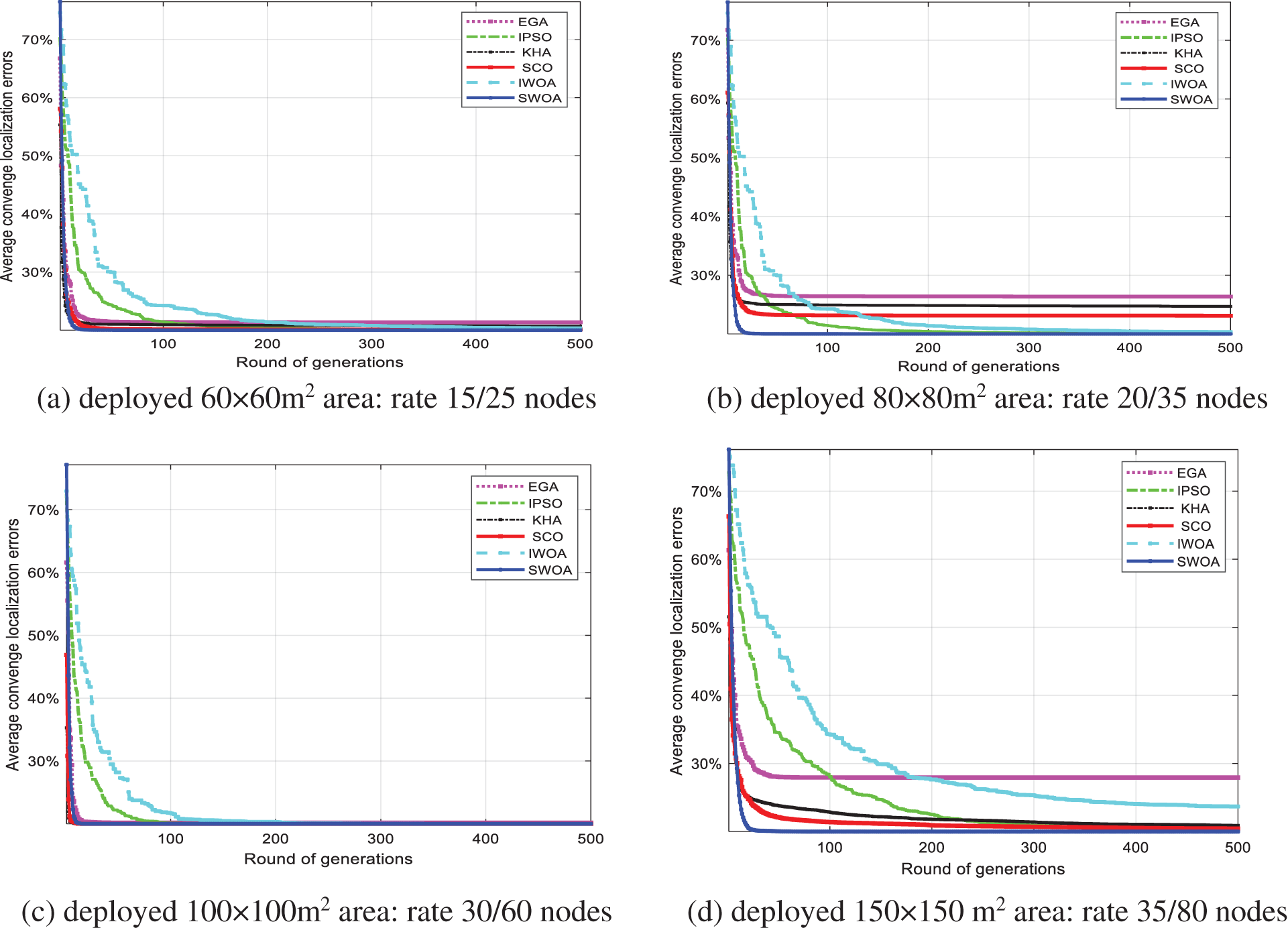
Figure 6: Convergence analysis of proposed node localization scheme in WSN compared against various optimizations, (a) deployed 60 × 60 m2 area: rate 15/25 nodes, (b) deployed 80 × 80 m2 area: rate 20/35 nodes, (c) deployed 100 × 100 m2 area: rate 30/60 nodes, and (d) deployed 150 × 150 m2 area: rate 35/80 nodes

It means that it tends to attain a higher convergence rate. The enhanced model effectively determines the position of the unknown node in WSN. It depicts the convergence evaluation of the proposed node localization approach over specific optimizations. The most cases, the superior belongs to the SWOA scheme. Hence, the lower value convergence tends to significantly improve the convergence rate to locate the sensor nodes in WSN.

The localization error analysis of localization errors of the proposed method compared with traditional algorithms concerning the variation of anchor nodes and sensor ranges. Fig. 7 shows the localization error analysis of the SWOA scheme compared against various algorithms for different scenarios of areas network deployment, e.g., (a) 60 × 60 m2, (b) 80 × 80 m2, (c) 100 × 100 m2, (d) 150 × 150 m2 setting, respectively.

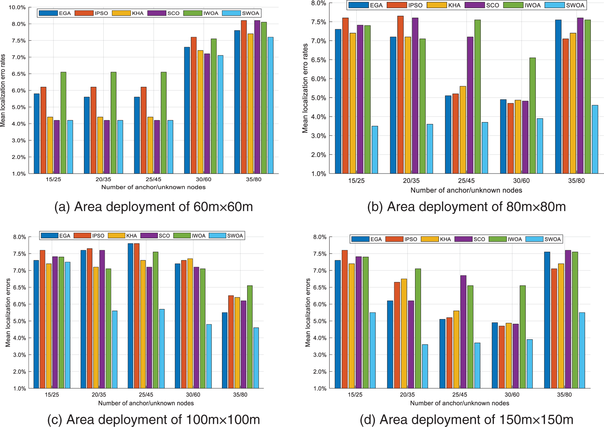
Figure 7: Localization error analysis of the SWOA node localization scheme compared against various algorithms for different scenarios of areas network deployment, e.g., (a) 60 × 60 m2, (b) 80 × 80 m2, (c) 100 × 100 m2, (d) 150 × 150 m2 setting, respectively

In most cases of setting net area deployments, the localization error analysis of the proposed SWOA scheme is smaller than the other schemes’ optimizations. In the error analysis with net deploying ranges of Fig. 7, the SWOA algorithm obtained the error output as less when compared to percentages of EGA around 1.5% to 3.2%, IPSO around 2.1% to 3.3%, KHA, around 1.5% to 4.2%, CSO around 2.5% to 5.2% around 2.5% to 4.6%, and IWOA around 1.5% to 5.1%. Similarly, Figs. 7b–7d represent the localization error analysis of the proposed scheme with varying unknown nodes. The error value achieved by the suggested SWOA algorithm is less localization error than the others in comparison as acquired to improve the localization performance over WSN.

Sensor nodes can exhaust their limited energy supply by performing computations and information transmission in a wireless environment without losing accuracy. Therefore, it is crucial to use energy-efficient communication and analytic methods. The battery life determines the lifespan of each sensor node, which serves as both a router and a data emitter. Its power outages or runs out cause some sensor nodes to malfunction, might have a substantial topological impact, and need packet rerouting and network reorganization.

The energy consumption during the receiving, demodulating, decapsulating, processing, encapsulating, modulating, transmission, and routing processes negatively affects network efficiency, which causes congestion and increases delays. The energy-aware routing involves the routing features, e.g., cluster formation, routing table, establish, and maintenance path. Due to its central significance in these functionalities, solutions are needed to reduce message broadcasting and beacon message exchange. The routing algorithm minimizes broadcast in environments with strict energy factor constraints. Packet sequencing is a popular method for resolving broadcast storm issues. The broadcast protocol should transport packets to all nodes in the network with the least amount of overhead, latency, and energy consumption possible.

In the Span method, the coordinator forms the message-forwarding backbone of the network. If two neighbors of a coordinator node cannot communicate directly or through one or more coordinators, the node should become a coordinator. Rotating coordinators show how localized node choices result in a connected, capacity-preserving global topology. As the ratio of idle-to-sleep energy consumption rises and grows with network density, the improvement in system lifespan due to Span increases. For instance, the simulations demonstrate that the system lifetime of an 802.11 network in power-saving mode with Span is two times better with a realistic energy model than without one. When used with the 802.11 power-saving methods, Span seamlessly interacts with the latter and enhances system longevity, capacity, and communication latency.

Table 5 compares the synthetic statistical analysis over parameters like errors, executed time, achieved converge at round generation, and average optimal converges that considered optimization algorithms with the other EGA, IPSO, KHA, SCO methods, and IWOA algorithms. It can be seen that the proposed SWOA has acquired a higher value than 1.5% to 4.6% for the EGA, 2.3% to 4.1% for the IPSO, 1.5% to 3.23% for the KHA, 1.7% to 4.1% for the SCO, and 2.3% to 4.1% for the IWOA algorithms in statistical analysis mean of the measured localization error, respectively.

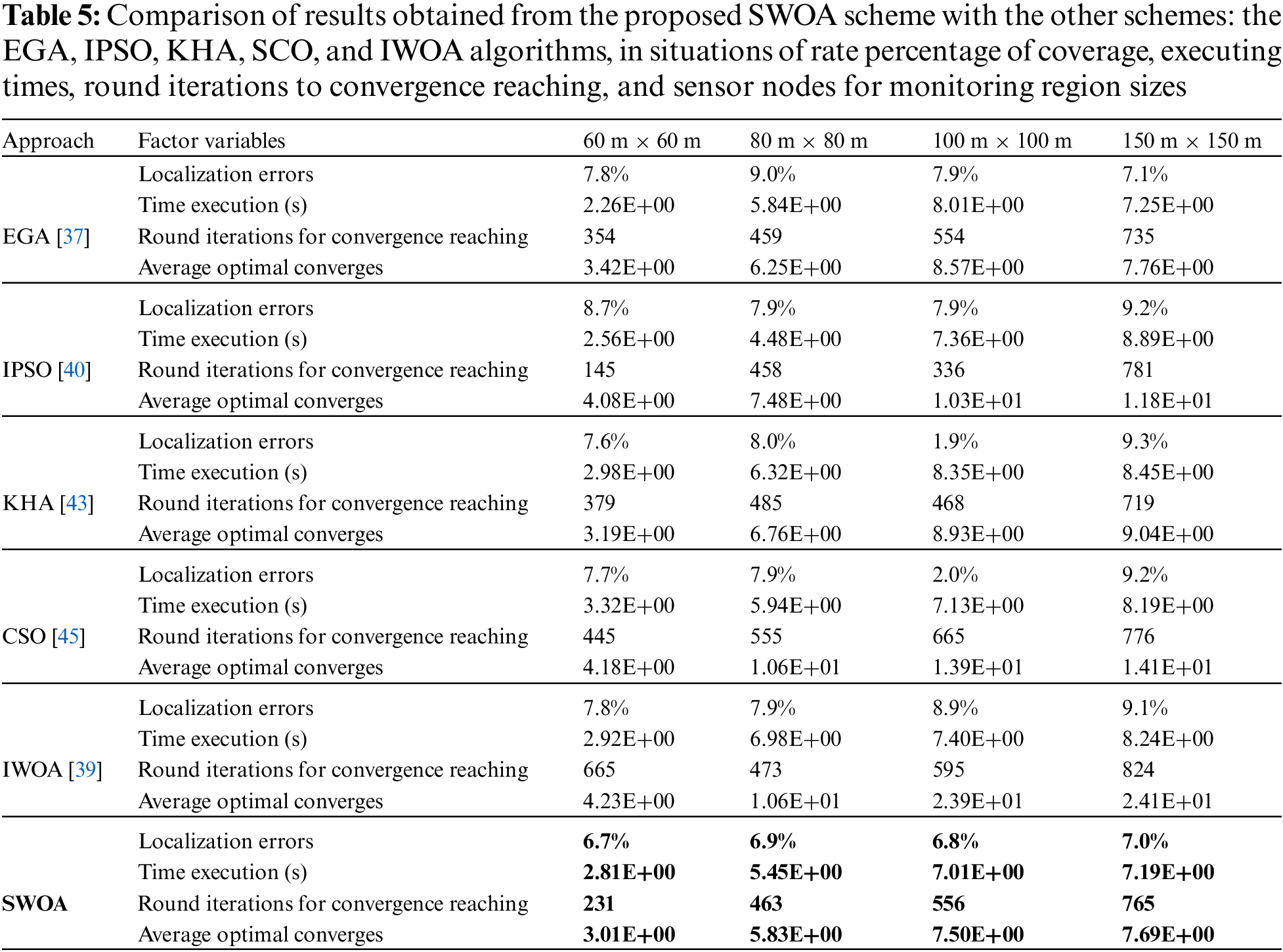
From the results, the statistical estimation of the recommended node localization model of the SWOA offers better performance in the cases of setting deployments than the other schemes’ optimizations. Significantly, the error and convergence values achieved by the SWOA are less location error, faster in convergence and executed time than the others compared to at least a reduced 1.5% to 4.7% error rate, and quicker by at least 4% and 2.1% in convergence and executed time, respectively for the experimental scenarios.

5  Conclusion

Because of the unsatisfactory performance of the traditional whale optimization algorithm (WOA), this paper proposed a siege whale optimization algorithm (SWOA) for the node localization scheme in WSN. The siege mechanism learned from the Harris Eagle optimization (HHO) algorithm was utilized to speed up whale hunting. An inertia weighting parameter was added at the end of each whale hunting iteration to control the update of the population position to prevent the update from stagnation. The mapped chaotic method generated the random initial population location to improve the algorithm’s ability and jump out of the local optimum. The SWOA algorithm was analyzed through function tests and node localization, compared with the other algorithms in the literature, which proved that the SWOA made significantly differs from the original algorithm. The core objective of the localization model is to determine the location of the unknown node in the WSN, considering variables like delay, path loss, energy, and received signal strength. The obtained optimal unknown node localization is provided with the help of the optimal value of the optimal solution in terms of position by the SWOA. The graph estimates the localization error with the objective function mathematically derived based on optimization from the SWOA. The simulation and performance are measured as convergence, and statistical analysis in the mean value of the proposed SWOA has acquired a higher value than 1.5% to 4.6% for the EGA, 2.3% to 4.1% for the IPSO, 1.5% to 3.23% for the KHA, 1.7% to 4.1% for the SCO, and 2.3% to 4.1% for the IWOA algorithms, respectively for some deployed area networks in terms of the measured localization error. Thus, the novel method can appropriately estimate the location of unknown nodes. In future work, the proposed algorithm could be applied to the broader use of WSN localizations in cloud computing, autonomous driving, the Internet of Things (IoT), and vectorized mapping. The placement can be established using vectorized road network maps and sensor data. Alternatively, the positioning is used for cloud-based crowdsourcing today and offers the self-services and other clients based on the information.

Acknowledgement: The authors would like to thank the editor and anonymous reviewers for their valuable suggestions and comments.

Funding Statement: This study was partially supported by the VNUHCM-University of Information Technology’s Scientific Research Support Fund.

Author Contributions: The authors confirm contribution to the paper as follows: conceptualization, T.T. Nguyen and T.K. Dao; methodology, T.T. Nguyen; software, T.K. Dao; validation, T.K. Dao, T.K. Dao and T.K. Dao; formal analysis, T.K. Dao; investigation, T.T. Nguyen; resources, T.K. Dao; writing—original draft preparation, T.K. Dao; writing—review and editing, T.T. Nguyen and T.K Dao; visualization, T.K. Dao; supervision, T.K. Dao; project administration, T.T. Nguyen; funding acquisition, T.K. Dao and T.T. Nguyen.

Availability of Data and Materials: Not applicable.

Conflicts of Interest: The authors declare that they have no conflicts of interest to report regarding the present study.

References

1. Shahraki, A., Taherkordi, A., Haugen, Q., Eliassen, F. (2020). Clustering objectives in wireless sensor networks: A survey and research direction analysis. Computer Networks, 180, 107376. https://doi.org/10.1016/j.comnet.2020.107376 [Google Scholar] [CrossRef]

2. Dao, T. K., Chu, S. C., Nguyen, T. T., Nguyen, T. D., Nguyen, V. T. (2022). An optimal WSN node coverage based on enhanced archimedes optimization algorithm. Entropy, 8(24), 1018. https://doi.org/10.3390/e24081018 [Google Scholar] [PubMed] [CrossRef]

3. Akyildiz, I. F., Su, W., Sankarasubramaniam, Y., Cayirci, E. (2002). A survey on sensor networks. IEEE Communications Magazine, 40(8), 102–105. https://doi.org/10.1109/MCOM.2002.1024422 [Google Scholar] [CrossRef]

4. Li, Y. S., Thai, M. T., Wu, W. L. (2008). Wireless sensor networks and applications. Springer New York, NY, USA: Springer Science and Business Media. [Google Scholar]

5. Raj, B., Ahmedy, I., Idris, M. Y. I., Noor, M. R. (2022). A survey on cluster head selection and cluster formation methods in wireless sensor networks. Wireless Communications and Mobile Computing, 2022(5), 5322649. https://doi.org/10.1155/2022/5322649 [Google Scholar] [CrossRef]

6. Nguyen, T. T., Pan, J. S., Dao, T. K. (2019). An improved flower pollination algorithm for optimizing layouts of nodes in wireless sensor network. IEEE Access, 7, 75985–75998. https://doi.org/10.1109/ACCESS.2019.2921721 [Google Scholar] [CrossRef]

7. Chen, X., Zhang, B. (2012). Improved DV-Hop node localization algorithm in wireless sensor networks. International Journal of Distributed Sensor Networks, 8(8), 213980. https://doi.org/10.1155/2012/213980 [Google Scholar] [CrossRef]

8. Shi, Q., He, C., Chen, H., Jiang, L. (2010). Distributed wireless sensor network localization via sequential greedy optimization algorithm. IEEE Transactions on Signal Processing, 58(6), 3328–3340. [Google Scholar]

9. Dao, T. K., Nguyen, T. T., Ngo, T. G., Nguyen, T. D. (2023). An optimal WSN coverage based on adapted transit search algorithm. International Journal of Software Engineering and Knowledge Engineering, 1–24. https://doi.org/10.1142/S0218194023400016 [Google Scholar] [CrossRef]

10. Farooqi, A. H., Khan, F. A. (2012). A survey of intrusion detection systems for wireless sensor networks. International Journal of Ad Hoc and Ubiquitous Computing, 9(2), 69–83. [Google Scholar]

11. Nguyen, T. T., Pan, J. S., Dao, T. K. (2019). A compact bat algorithm for unequal clustering in wireless sensor networks. Applied Sciences, 9(10), 1973. https://doi.org/10.3390/app9101973 [Google Scholar] [CrossRef]

12. Vecchio, M., López-Valcarce, R., Marcelloni, F. (2012). A two-objective evolutionary approach based on topological constraints for node localization in wireless sensor networks. Applied Soft Computing Journal, 12(7), 1891–1901. https://doi.org/10.1016/j.asoc.2011.03.012 [Google Scholar] [CrossRef]

13. Wang, J., Ghosh, R. K., Das, S. K. (2010). A survey on sensor localization. Journal of Control Theory and Applications, 8, 2–11. https://doi.org/10.1007/s11768-010-9187-7 [Google Scholar] [CrossRef]

14. Arora, S., Singh, S. (2017). Node localization in wireless sensor networks using butterfly optimization algorithm. Arabian Journal for Science and Engineering, 42(8), 3325–3335. https://doi.org/10.1007/s13369-017-2471-9 [Google Scholar] [CrossRef]

15. Nguyen, T. T., Thom, H. T. H., Dao, T. K. (2017). Estimation localization in wireless sensor network based on multi-objective grey wolf optimizer. Advances in Information and Communication Technology: Proceedings of the International Conference, pp. 228–237. Thai Nguyen, Vietnam. [Google Scholar]

16. Kulkarni, V. R., Desai, V., Kulkarni, R. V. (2019). A comparative investigation of deterministic and metaheuristic algorithms for node localization in wireless sensor networks. Wireless Networks, 25, 2789–2803. [Google Scholar]

17. Sivakumar, S., Venkatesan, R. (2015). Meta-heuristic approaches for minimizing error in localization of wireless sensor networks. Applied Soft Computing, 36, 506–518. [Google Scholar]

18. Srinivas, M., Patnaik, L. M. (1994). Genetic algorithms: A survey. Computer, 27(6), 17–26. https://doi.org/10.1109/2.294849 [Google Scholar] [CrossRef]

19. Koulamas, C., Antony, S. R., Jaen, R. (1994). A survey of simulated annealing applications to operations research problems. Omega, 22(1), 41–56. [Google Scholar]

20. Szu, H., Hartley, R. (1987). Fast simulated annealing. Physics Letters A, 122, 157–162. https://doi.org/10.1016/0375-9601(87)90796-1 [Google Scholar] [CrossRef]

21. Kennedy, J., Eberhart, R. (1995). Particle swarm optimization. Proceedings of ICNN’95-International Conference on Neural Networks, vol. 6, no. 4, pp. 1942–1948. Perth, WA, Australia. https://doi.org/10.1109/ICNN.1995.488968 [Google Scholar] [CrossRef]

22. Mirjalili, S., Lewis, A. (2016). The whale optimization algorithm. Advances in Engineering Software, 95, 51–67. https://doi.org/10.1016/j.advengsoft.2016.01.008 [Google Scholar] [CrossRef]

23. Heidari, A. A., Mirjalili, S., Faris, H., Aljarah, I., Mafarja, M. et al. (2019). Harris hawks optimization: Algorithm and applications. Future Generation Computer Systems, 97, 849–872. https://doi.org/10.1016/j.future.2019.02.028 [Google Scholar] [CrossRef]

24. Mirjalili, S. (2015). The ant lion optimizer. Advances in Engineering Software, 83, 80–98. https://doi.org/10.1016/j.advengsoft.2015.01.010 [Google Scholar] [CrossRef]

25. Mirjalili, S. (2015). Moth-flame optimization algorithm: A novel nature-inspired heuristic paradigm. Knowledge-Based Systems, 89, 228–249. [Google Scholar]

26. Mirjalili, S., Mirjalili, S. M., Lewis, A. (2014). Grey wolf optimizer. Advances in Engineering Software, 69, 46–61. https://doi.org/10.1016/j.advengsoft.2013.12.007 [Google Scholar] [CrossRef]

27. Rana, N., Latiff, M. S. A., Abdulhamid, S. M., Chiroma, H. (2020). Whale optimization algorithm: A systematic review of contemporary applications, modifications and developments. Neural Computing and Applications, 32(20), 16245–16277. https://doi.org/10.1007/s00521-020-04849-z [Google Scholar] [CrossRef]

28. Mirjalili, S., Mirjalili, S. M., Saremi, S., Mirjalili, S. (2020). Whale optimization algorithm: Theory, literature review, and application in designing photonic crystal filters. In: Mirjalili, S., Song Dong, J., Lewis, A. (Eds.BT-nature-inspired optimizers: Theories, literature reviews and applications, pp. 219–238. Cham: Springer International Publishing. [Google Scholar]

29. Sun, W., Zhang, C. (2018). Analysis and forecasting of the carbon price using multi—resolution singular value decomposition and extreme learning machine optimized by adaptive whale optimization algorithm. Applied Energy, 231, 1354–1371. https://doi.org/10.1016/j.apenergy.2018.09.118 [Google Scholar] [CrossRef]

30. Chakraborty, S., Saha, A. K., Chakraborty, R., Saha, M. (2021). An enhanced whale optimization algorithm for large scale optimization problems. Knowledge-Based Systems, 233, 107543. https://doi.org/10.1016/j.knosys.2021.107543 [Google Scholar] [CrossRef]

31. Bozorgi, S. M., Yazdani, S. (2019). IWOA: An improved whale optimization algorithm for optimization problems. Journal of Computational Design and Engineering, 6, 243–259. https://doi.org/10.1016/j.jcde.2019.02.002 [Google Scholar] [CrossRef]

32. Sun, Y., Wang, X., Chen, Y., Liu, Z. (2018). A modified whale optimization algorithm for large-scale global optimization problems. Expert Systems with Applications, 114, 563–577. https://doi.org/10.1016/j.eswa.2018.08.027 [Google Scholar] [CrossRef]

33. Wolpert, D. H., Macready, W. G. (1997). No free lunch theorems for optimization. IEEE Transactions on Evolutionary Computation, 1(1), 67–82. https://doi.org/10.1109/4235.585893 [Google Scholar] [CrossRef]

34. Yang, X. S. (2011). Metaheuristic optimization: Algorithm analysis and open problems. Experimental Algorithms: 10th International Symposium, SEA 2011, vol. 10, pp. 21–32. Kolimpari, Chania, Crete, Greece. [Google Scholar]

35. Nguyen, T. T., Pan, J. S., Chu, S. C., Roddick, J. F., Dao, T. K. (2016). Optimization localization in wireless sensor network based on multi-objective firefly algorithm. Journal of Network Intelligence, 1(4), 130–138. [Google Scholar]

36. Najarro, L. A. C., Song, I., Kim, K. (2022). Fundamental limitations and state-of-the-art solutions for target node localization in WSNs: A review. IEEE Sensors Journal, 22(24), 23661–23682. https://doi.org/10.1109/JSEN.2022.3217335 [Google Scholar] [CrossRef]

37. Ren, Q., Zhang, Y., Nikolaidis, I., Li, J., Pan, Y. (2020). RSSI quantization and genetic algorithm based localization in wireless sensor networks. Ad Hoc Networks, 107, 102255. https://doi.org/10.1016/j.adhoc.2020.102255 [Google Scholar] [CrossRef]

38. Shakila, R., Paramasivan, B. (2021). RETRACTED ARTICLE: An improved range based localization using whale optimization algorithm in underwater wireless sensor network. Journal of Ambient Intelligence and Humanized Computing, 12(6), 6479–6489. https://doi.org/10.1007/s12652-020-02263-w [Google Scholar] [CrossRef]

39. Gou, P., He, B., Yu, Z. (2021). A node location algorithm based on improved whale optimization in wireless sensor networks. Wireless Communications and Mobile Computing, 2021, 1–17. https://doi.org/10.1155/2021/3927584 [Google Scholar] [CrossRef]

40. Phoemphon, S., So-In, C., Leelathakul, N. (2020). A hybrid localization model using node segmentation and improved particle swarm optimization with obstacle-awareness for wireless sensor networks. Expert Systems with Applications, 143, 113044. https://doi.org/10.1016/j.eswa.2019.113044 [Google Scholar] [CrossRef]

41. Lakshmi, Y. V., Singh, P., Abouhawwash, M., Mahajan, S., Pandit, A. K. et al. (2022). Improved chan algorithm based optimum UWB sensor node localization using hybrid particle swarm optimization. IEEE Access, 10, 32546–32565. https://doi.org/10.1109/ACCESS.2022.3157719 [Google Scholar] [CrossRef]

42. Nithya, B., Jeyachidra, J. (2021). Hybrid ABC-BAT optimization algorithm for localization in HWSN. Microprocessors and Microsystems, S0141-9331(21)00197-6. https://doi.org/10.1016/j.micpro.2021.104024 [Google Scholar] [CrossRef]

43. Sabbella, V. R., Edla, D. R., Lipare, A., Parne, S. R. (2021). An efficient localization approach in wireless sensor networks using krill herd optimization algorithm. IEEE Systems Journal, 15(2), 2432–2442. https://doi.org/10.1109/JSYST.2020.3004527 [Google Scholar] [CrossRef]

44. Kulkarni, R. V., Venayagamoorthy, G. K. (2010). Bio-inspired algorithms for autonomous deployment and localization of sensor nodes. IEEE Transactions on Systems Man & Cybernetics Part C (Applications and Reviews), 40(6). [Google Scholar]

45. Al Shayokh, M., Shin, S. Y. (2017). Bio inspired distributed WSN localization based on chicken swarm optimization. Wireless Personal Communications, 97, 5691–5706. [Google Scholar]

46. Nguyen, T. T., Pan, J. S., Dao, T. K., Sung, T. W., Ngo, T. G. (2020). Pigeon-inspired optimization for node location in wireless sensor network. In: Sattler, K. U., Nguyen, D., Vu, N., Tien Long, B., Puta, H. (Eds.Advances in engineering research and application, vol. 104. Cham: Springer. https://doi.org/10.1007/978-3-030-37497-6_67 [Google Scholar] [CrossRef]

47. Cheung, K. W., So, H. C., Ma, W. K., Chan, Y. T. (2004). Least squares algorithms for time-of-arrival-based mobile location. IEEE Transactions on Signal Processing, 52, 1121–1130. [Google Scholar]

48. Chen, H., Li, W., Yang, X. (2020). A whale optimization algorithm with chaos mechanism based on quasi-opposition for global optimization problems. Expert Systems with Applications, 158, 113612. https://doi.org/10.1016/j.eswa.2020.113612 [Google Scholar] [CrossRef]

49. Elaziz, M. A., Mirjalili, S. (2019). A hyper-heuristic for improving the initial population of whale optimization algorithm. Knowledge-Based Systems, 172, 42–63. https://doi.org/10.1016/j.knosys.2019.02.010 [Google Scholar] [CrossRef]

50. Chen, B., Jamieson, K., Balakrishnan, H., Morris, R. (2002). Span: An energy-efficient coordination algorithm for topology maintenance in ad hoc wireless networks. Wireless Networks, 8(5), 481–494. https://doi.org/10.1023/A:1016542229220 [Google Scholar] [CrossRef]

Appendix A.

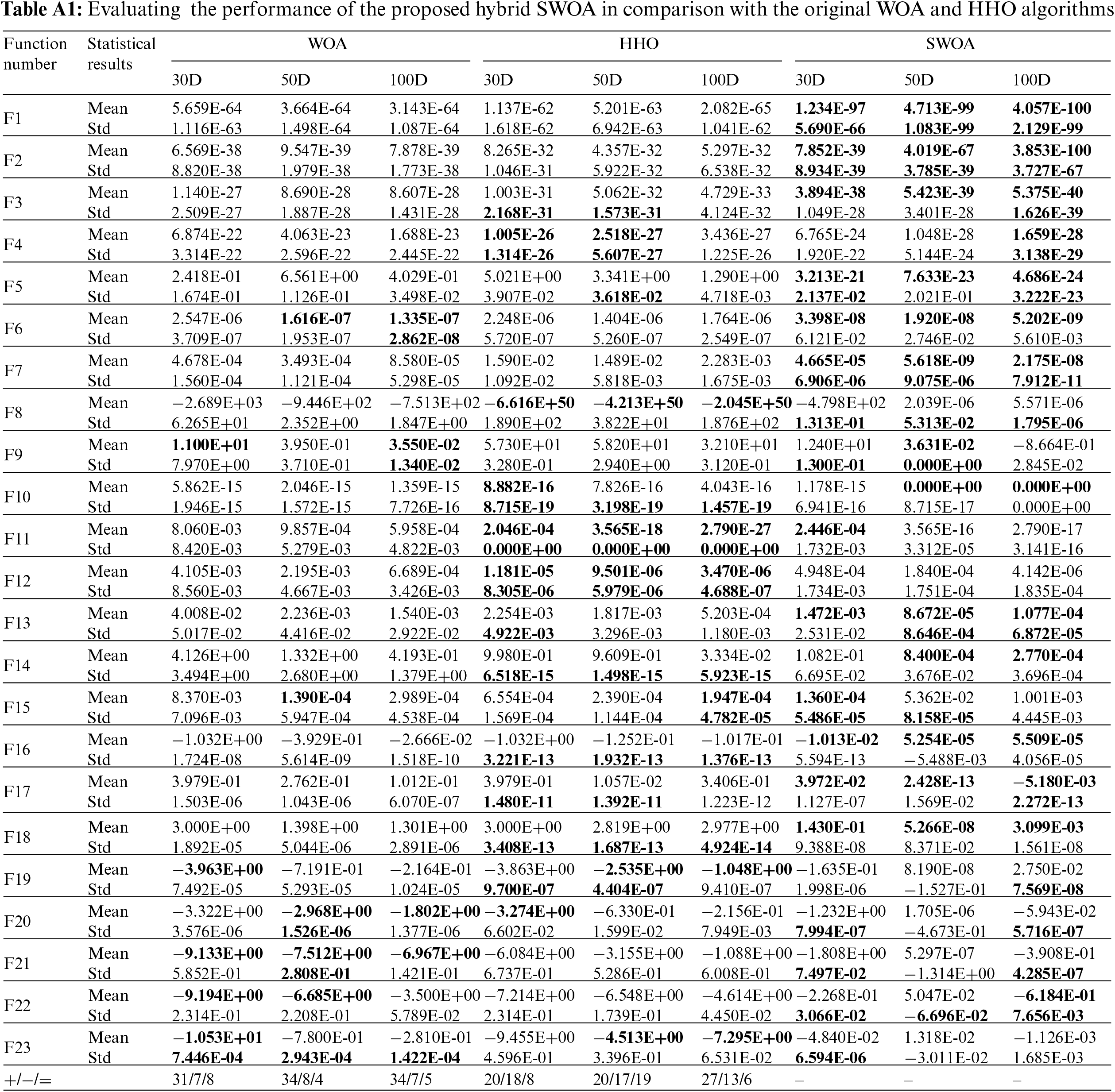
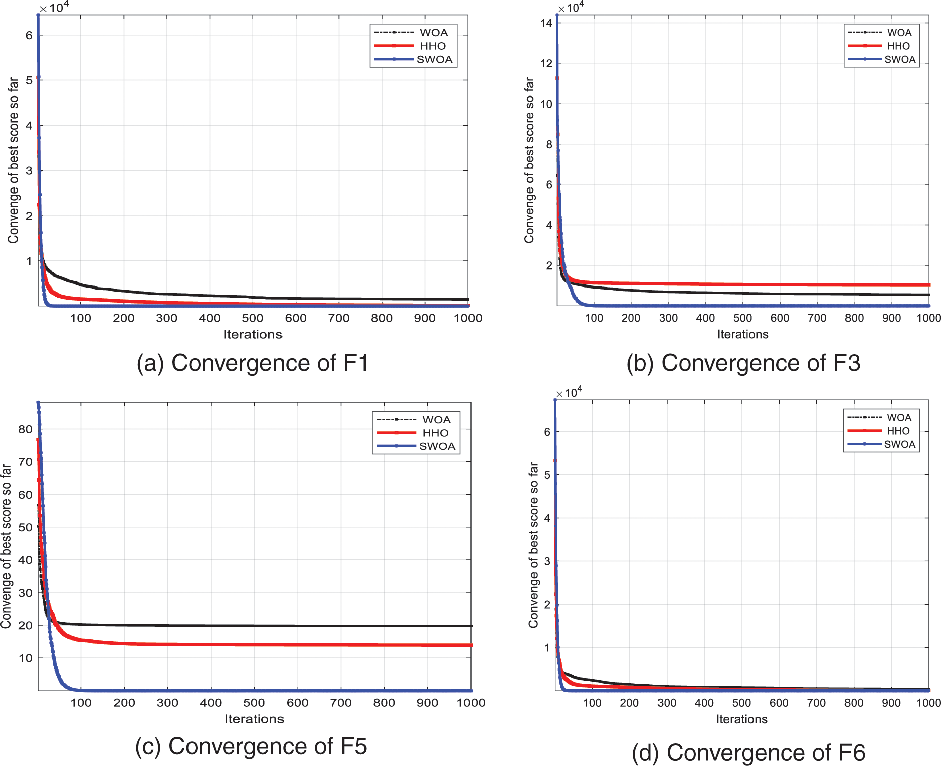
Figure A1: Comparison of the converge curves of the SWOA with the original WOA and HHO algorithms for the selected functions: (a) F1, (b) F3, (c) F5, and (d) F6

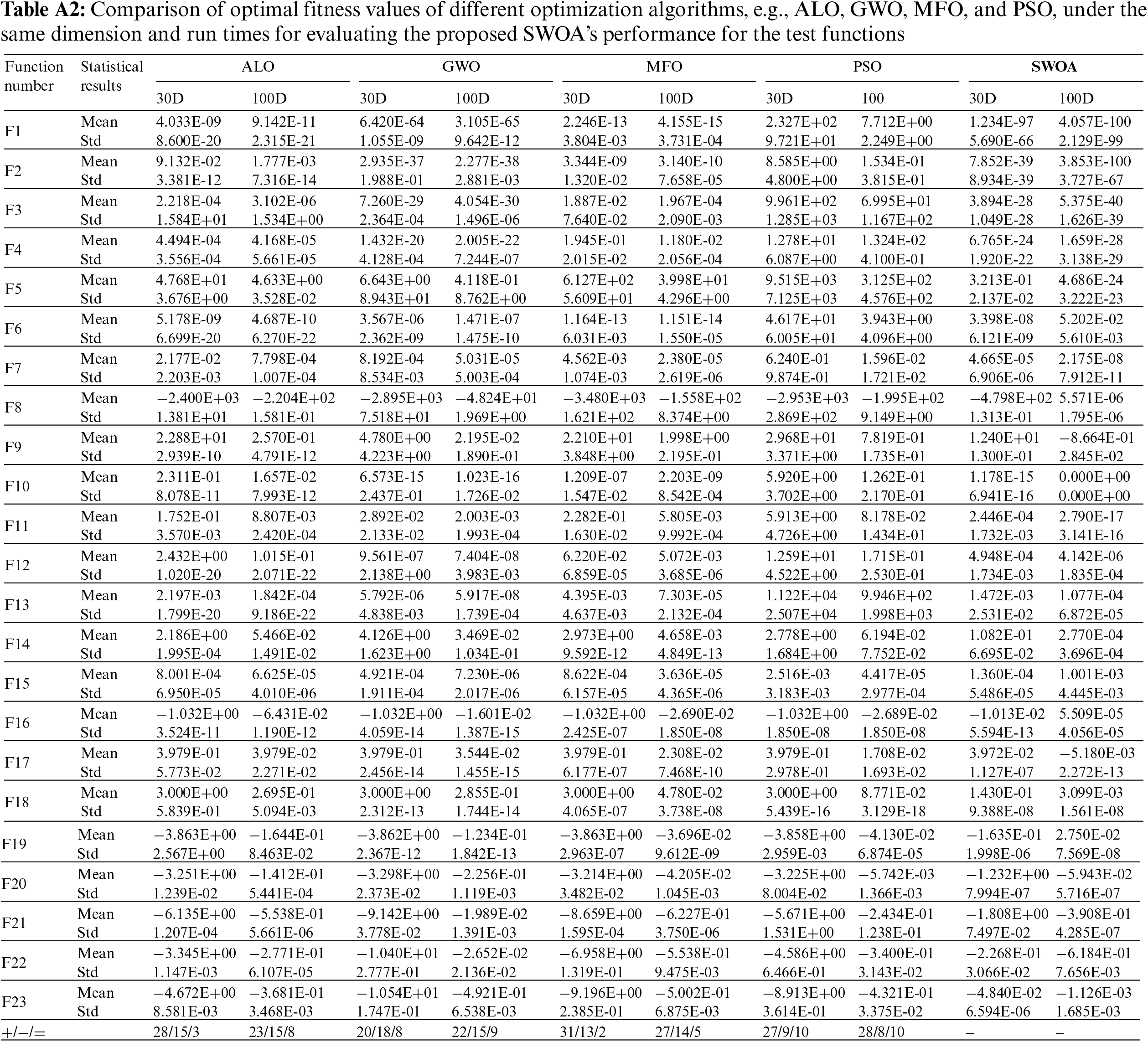
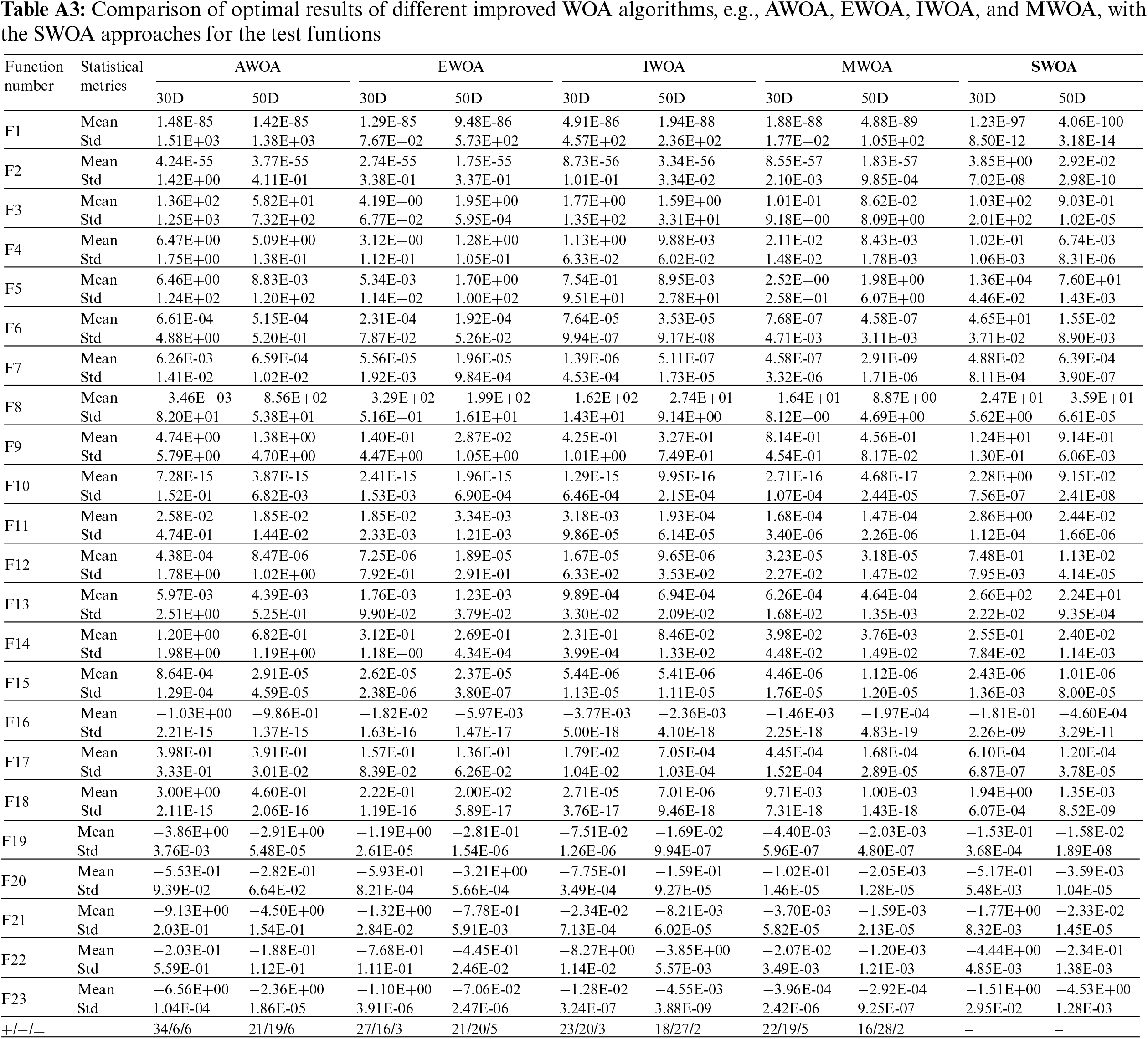
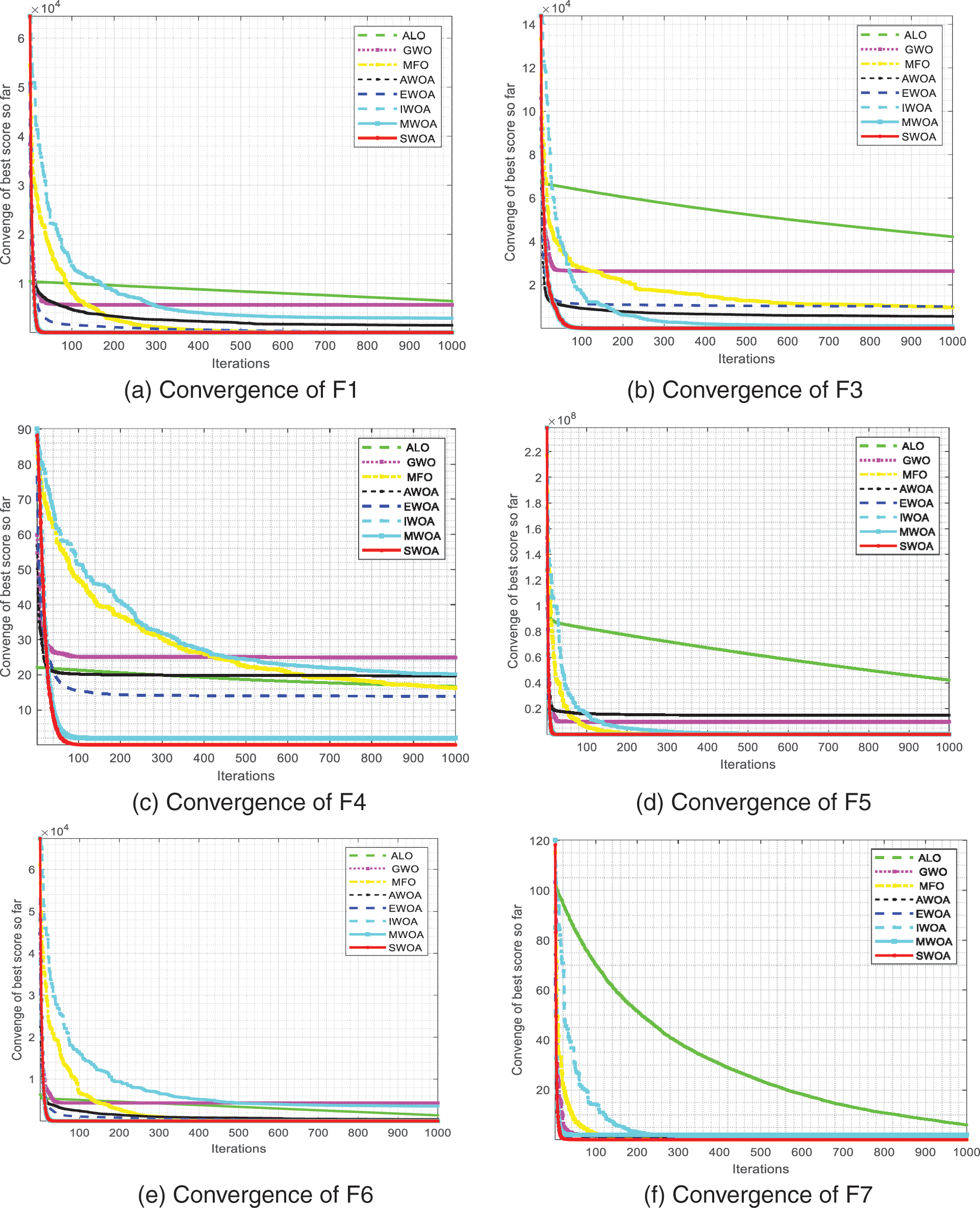
Figure A2: Comparison of the converge curves of the proposed SWOA with the ALO, GWO, MFO, AWOA, EWOA, IWOA, and MWOA algorithms for the selected functions (a) F1, (b) F3, (c) F4, (d) F5, (e) F6, (f) F7, (g) F11, (h) F13