Optimization of Center of Gravity Position and Anti-Wave Plate Angle of Amphibious Unmanned Vehicle Based on Orthogonal Experimental Method

1  Introduction

The amphibious vehicle is a kind of equipment with both land and water maneuvering ability [1]. Because of its amphibious maneuvering ability, it is widely used in agriculture and fishery, military, tourism, and other fields. When studying the navigation characteristics of amphibious vehicles, the resistance characteristics of different types of amphibious vehicles vary with the driving speed. There are three states of navigation according to the volumetric Froude number (Fr) of the vehicle’s speed, when Fr < 1.0, it is the drainage sailing state; when Fr>3.0, it is the gliding state; the other state is the transition sailing state. Due to the amphibious vehicles that need to be driven on land, their shape structure is complex, which is significantly different from the streamlined shape of ships. Moreover, the blunt structure leads to a high coefficient of squareness, and the resistance characteristics of amphibious vehicles during navigation are also greatly different from those of ships. The surrounding flow field is prone to a large number of separations, and the phenomenon of wave generating and turbulence is serious. Installing accessories on the vehicle body, such as anti-wave plates and tail slide boards, can optimize the underwater driving performance without changing the vehicle’s structure. Many amphibious vehicles at home and abroad are equipped with anti-wave plates in the front of the vehicle to reduce driving resistance.

The towing experiment of the amphibious vehicle based on Froude’s similarity theory can monitor the resistance and driving attitude of the vehicle, which is reliable and mature in application but is costly and difficult to simulate a variety of working conditions. With the development of computer technology, the application of Computational Fluid Dynamics (CFD) technology has greatly assisted the study of amphibious equipment. Numerical methods can be applied to study the hydrodynamic characteristics of amphibious vehicles traveling in water. The combination of modeling tests and numerical calculations is an effective way to study the water performance of wheeled amphibious vehicles. CFD can make up for the shortcomings of the model test, not only calculating a variety of working conditions more accurately but also accurately capturing the details of the flow field, from the essence of the fluid flow to consider the elements affecting the hydrodynamic performance of amphibious vehicles, and then put forward the optimization measures of the vehicle body. The use of computer simulation software to establish a “digital pool”, and simulate amphibious vehicle navigation in real waters in a computerized virtual watershed not only can easily simulate a variety of sailing conditions but also capture data such as the flow field around the vehicle and the force on the vehicle structure, which is convenient for researchers to conduct in-depth analysis in the subsequent optimization design [2–5]. More et al. [6] analyzed the stability and resistance of a wheeled amphibious fighting vehicle through a combination of model tests and numerical calculations, which provides a reference for amphibious vehicle shape design. Xu et al. [7] designed the wheel-retracting mechanism to reduce the resistance and increase speed for a high-speed wheeled amphibious vehicle and used the CFD numerical method to research the influence. Demirel et al. [8] proposed a CFD numerical model that enabled the prediction of the effect of antifouling coatings on frictional resistance.

The related optimization research of amphibious vehicles can be roughly divided into two parts: the study of hydrodynamic performance of navigation and the driving path planning. In path planning research, some scholars used relative algorithms to realize path planning and make the vehicle more adaptable to different navigation environments [9–11]. Meanwhile, the hydrodynamic performance of the amphibious vehicle is an important factor that affects the underwater navigation characteristics. This paper focused on the research of hydrodynamic performance of the amphibious vehicle underwater navigation.

Many researchers focus on the influence of vehicle shape or trim angle on navigation characteristics when studying the hydrodynamics of drainage amphibious vehicles, i.e., to reduce navigation resistance by optimizing shape or driving attitude [12–14]. Some scholars have studied the navigation characteristics of amphibious vehicles with anti-wave plates in the front of the vehicle, but only the effects of whether or not to add anti-wave plates on the navigational characteristics [15,16]. Few scholars have studied the influence of the angle of the plate on the navigation characteristics of amphibious vehicles, and other factors affecting navigation characteristics, such as center of gravity was not considered at the same time. Several scholars have studied the center of gravity of vehicles, which is adjusted to improve navigation characteristics. A small-sized high-maneuverable remotely operated vehicle with a Variable Center of Gravity (VCG) system was designed and implemented by Tolstonogov et al. [17]. It can be seen that the position of the center of gravity has a great effect on the navigation characteristics.

Summarizing the previous related research, in terms of grid division, if a static grid is applied for numerical calculation, the calculation is easy to converge, and the grid division is relatively simple, but because of the change of the flow field when the amphibious vehicle is traveling, not only the accuracy of the calculation results cannot be guaranteed, but also the adjustment steps of the vehicle’s attitude are very cumbersome and inefficient. The dynamic grid used in this paper effectively avoids the above problems. Regarding the selection of optimization factors, the previous studies on the angle of the anti-wave plate were relatively simple, the parameter selection was simple and unscientific, and the most important thing was that the influence of the center of gravity position was not considered at the same time. Therefore, when studying the resistance reduction characteristics of amphibious vehicles, the influence laws of the angle of the anti-wave plate and the position of the center of gravity should be considered at the same time.

This paper is based on the fluid dynamics theory and the numerical calculation model of the amphibious unmanned vehicle was established by using VOF and Dynamic Fluid Body Interaction (DFBI) methods. The numerical calculation results were compared with the towing test values to verify the validity of the model. Based on this model, the influence of the center of gravity position on the resistance characteristics was investigated, and orthogonal tables were used to group the angle of the anti-wave plate as well as the position of the center of gravity, to study the influence of the combination of the above factors on the navigation resistance and driving stability.

2  Numerical Calculation Method

2.1 Numerical Calculation Model

The resistance of amphibious vehicles in water is mainly composed of friction resistance, wave resistance, and shape resistance. Among them, friction resistance is formed by the friction between water and the surface of the vehicles. Water flowing through the moving vehicles produces waves, forming a pressure difference and thus generating wave resistance. When the amphibious vehicle is traveling, due to the influence of the shape and the speed of the water flow, the water pressure at different positions on the vehicle’s surface is different, leading to a pressure difference, thus forming shape resistance. In computer simulation software, friction resistance and pressure resistance can be directly monitored, and the sum of the two is the total resistance. Pressure resistance includes shape and wave resistance, so all resistance data can be obtained by obtaining one. The sum of friction resistance and shape resistance is also called viscous resistance. After the total resistance of the amphibious vehicle is obtained, the free surface is set as a symmetric plane and the influence of free surface wave generation is eliminated to obtain viscous resistance, and then wave generation resistance is obtained by subtracting viscous resistance from total resistance.

The free surface flow around the amphibious vehicle is a two-phase flow problem. The free surface is the interface between water and air. In this paper, STAR-CCM+ software is used for numerical calculation, and a mathematical model of the flow field around amphibious unmanned vehicles is established based on computational fluid dynamics theory. The water and air in the virtual watershed are assumed to be incompressible fluids. The Finite Volume Method (FVM) is used for spatial dispersion, and the free liquid surface is captured by the VOF method [18,19]. The simulation is completed in the model area by defining VOF waves at the velocity inlet boundary to simulate the incoming velocity and liquid level height, simulating the linear motion of the vehicle in the water as well as specifying the free liquid level. In the simulation, the main input parameters are speed, vehicle weight, center of gravity position, and moment of inertia around the y-axis of the center of gravity position. Since the simulation simulates the navigation of the amphibious vehicle in still water, it is not necessary to define the VOF wave function. After the simulation, the navigation resistance and vehicle trim angle parameter curves are output.

The k-ε turbulence model [20] proposed by Launder and Spalding is chosen as the turbulence model. This model can be used to deal with complex turbulence problems and has been widely used in the field of amphibious vehicle simulation. Wang et al. [21] compared the drag data from numerical calculations and towing tests to verify the effectiveness of using the k-ε turbulence model in the numerical simulation of amphibious vehicles.

The motion of the amphibious vehicle is a transient problem, so an implicit non-stationary solver is used to solve the fluid equations.

Based on the above model, the flow field around the amphibious unmanned vehicle is as follows:

Continuity equation

∂ρ∂t+∂ρui∂xi=0(1)

The turbulent kinetic energy k-equation and the turbulent dissipation rate ε-equation are expressed as:

The k-equation

∂(ρk)∂t+∂(ρuik)∂xi=∂∂xi[(μ+μtσk)∂k∂xi]+G−ρε(2)

The ε-equation

∂(ρε)∂t+∂(ρuiε)∂xi=∂∂xi[(μ+μtσε)∂ε∂xi]+C1εεkG−C2ερε2k(3)

where k is the turbulent kinetic energy. ε is the turbulent dissipation rate. ui is the velocity component. xi is the coordinate component, t is the time. μ is the viscosity coefficient. μt is the turbulent viscosity coefficient. ρ is the density. σk and σε are the turbulence Prandtl numbers for turbulence kinetic energy k and turbulence dissipation rate ε, respectively. σk = 1.0, σε = 1.3; C1ε = 1.44, C2ε = 1.92, G is the generation term of turbulent kinetic energy k.

STAR-CCM+ DFBI module is used to simulate the motion attitude of an amphibious unmanned vehicle. By loading the DFBI module, the motion attributes of the amphibious unmanned vehicle are defined, and the two degrees of freedom, pitch and heave are released to realize the dynamic monitoring of the vehicle’s attitude during the simulation.

To improve the stability of the calculation, the release time and the buffer time can be defined to avoid the body moving before the flow field is stabilized at the beginning of the calculation, and at the same time to reduce the impact effect of the fluid on the vehicle.

The form factor of the amphibious unmanned vehicle is shown in Fig. 1. Among them, the length, width, and height dimensions of the main body are 1600 mm × 800 mm × 622 mm, respectively. When driving on land, the four wheels of the amphibious unmanned vehicle are driven by four 750 W servo DC motors. Underwater navigation is powered by a vector thruster mounted at the rear of the vehicle, which is driven by a 5 kW motor with an impeller speed of 3000 r/min. The total weight of the unmanned vehicle is 242 kg. The anti-wave plate is segmented and the angle can be adjusted.

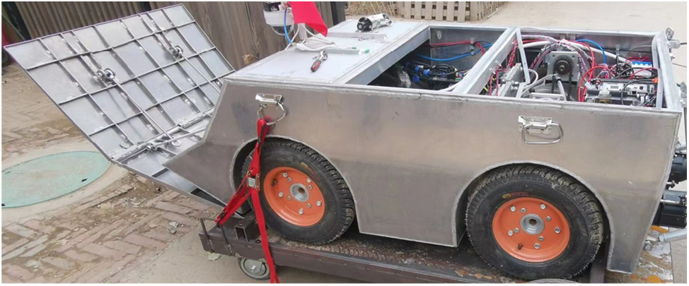
Figure 1: Form factor of amphibious unmanned vehicle

According to the shape and structure of the amphibious unmanned vehicle, the 3D model was simplified, and the simplified model is shown in Fig. 2.

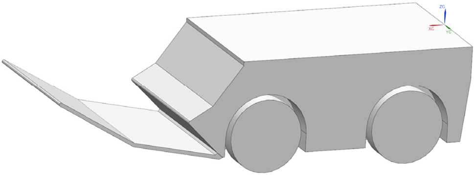
Figure 2: Simplified model of amphibious unmanned vehicle

2.2 Grid Division and Boundary Conditions

2.2.1 Grid Division

Grid division is an important step in simulation pre-processing. In this paper, the overlapping grid [22,23] technique was used to divide the entire computational area into the background area and overset area. The overset area will move with the movement of the research object, and the data exchange between the two types of grid areas is realized by defining the overlapping grid interface. The computational domain using this method will not distort and deform between the grids when the object is moving, which ensures high precision and makes the computational process less likely to diverge.

The amphibious unmanned vehicle generates Kelvin waves as it navigates through the water, and the flow field in the free surface changes dramatically due to the changes in the vehicle’s attitude. Therefore, it was necessary to reasonably divide the grid of the computing domain according to the structure of the amphibious unmanned vehicle and the force characteristics in the flow field and encrypt the grid near the water-free surface perpendicular to the direction of the flow field. To save computational resources, the size of the background grid was set to be larger, and two sets of transition grids were set at the same time to reduce the interaction error between grids and thus reduce the computational error. Some key locations such as anti-wave plates and vehicle surfaces also needed to be properly encrypted. The grid division of the watershed near the amphibious unmanned vehicle body is shown in Fig. 3.

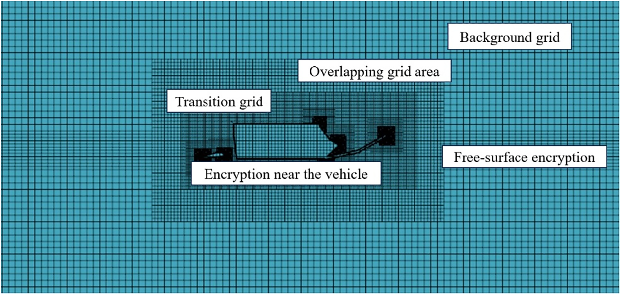
Figure 3: The grid near the vehicle

2.2.2 Boundary Condition

The appropriate watershed size can improve computational efficiency while adequately representing the flow field around the unmanned vehicle. The numerically computed watersheds are constructed as shown in Fig. 4, and the whole watershed is a symmetric half-mode. L is the length of the amphibious unmanned vehicle. The driving direction of the unmanned vehicle is the positive direction of the x-axis, the vertical upward direction of the vehicle is the positive direction of the z-axis, and the vertical left side of the vehicle is the positive direction of the y-axis. The origin is located at the end of the top surface of the vehicle, passing through the symmetric plane of the watershed. Assuming that the amphibious unmanned vehicle does not move, it is set as a fixed reference system. Setting the inlet velocity, the water flows from the velocity inlet directly in front of the watershed to the direction of the vehicle, and the surface of the vehicle body is set as a non-slip wall. In the process of numerical simulation, large mesh size transition and boundary will cause wave reflection. To eliminate its effect on the simulation results, the damping wave reflection option was turned on in the boundary conditions of the front velocity inlet, side velocity inlet, and pressure outlet, and the length was taken as 1.5 times the length of the vehicle.

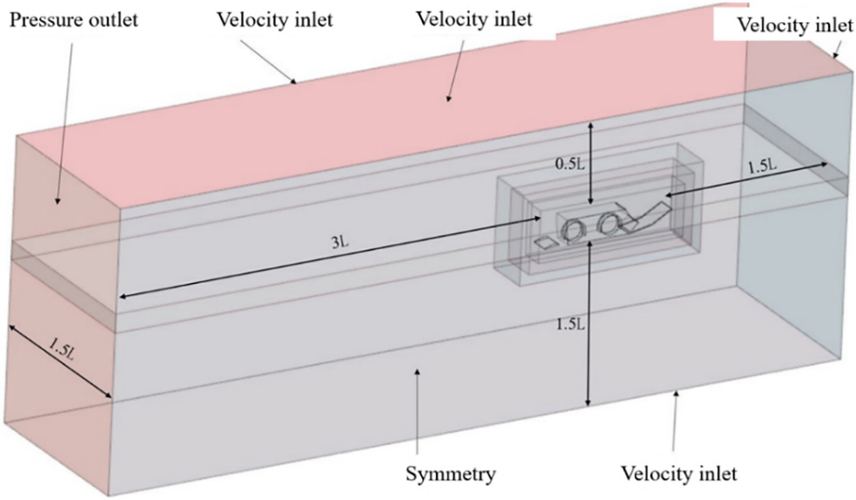
Figure 4: Setting of watershed boundary conditions

2.3 Numerical Uncertainty Analysis

In numerical calculation, appropriate grid numbers and time steps can ensure the accuracy of the calculation results and improve the calculation efficiency. Based on the same boundary conditions, the number of global grids and the time steps were adjusted for numerical calculation to verify the influence on the resistance data.

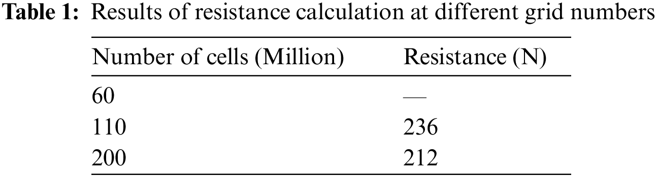
Grid independence analysis: Compared the effects of three numerical models with different grid numbers on the results of resistance calculation for amphibious unmanned vehicle driving at a speed of 2 m/s, the number of grids selected is 600,000, 1.1 million and 2 million. The calculation results are shown in Table 1. When the number of grids is 600,000, the size of the global basic grid increases, which is greatly different from the grid size of the flow field around the vehicle. Therefore, the flow field around the unmanned vehicle cannot be accurately expressed, and the numerical calculation results cannot converge. Once the number of grids exceeds 1.1 million, continued encryption of the grid has little effect on the resistance values. Therefore, to ensure the efficiency of numerical computation, this paper adopts the grid numbers of 1.1 million for subsequent calculations to meet the requirements.

Time step independence analysis: Used a numerical model with a total number of grids of 1.1 million, the effects of time steps of 0.01, 0.02, and 0.03 s on the resistance calculation results were compared at a traveling speed of 2 m/s. The calculation results are shown in Table 2.

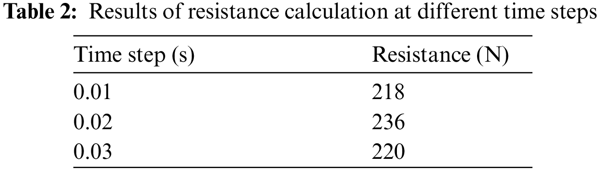
From the calculation results, it can be seen that the sensitivity of this numerical computation model to the three selected time steps is low, and to ensure the efficiency of numerical computation, the time step is selected 0.02 s.

3  Analysis of Numerical Calculation Results

3.1 The Validity of Numerical Models

The towing test of the amphibious unmanned vehicle was accomplished in the towing pool of Huazhong University of Science and Technology (HUST), which has a length, width, and depth of 175, 6, and 4 m, respectively. The vehicle’s waterline is 0.322 m and the speed range of the trailer is 0.01~8 m/s. The speed accuracy is ±1 mm/s. The drag test method was carried out according to the CB/Z 244-2018 Test method for model resistance of planning craft. The towing test site is shown in Fig. 5.

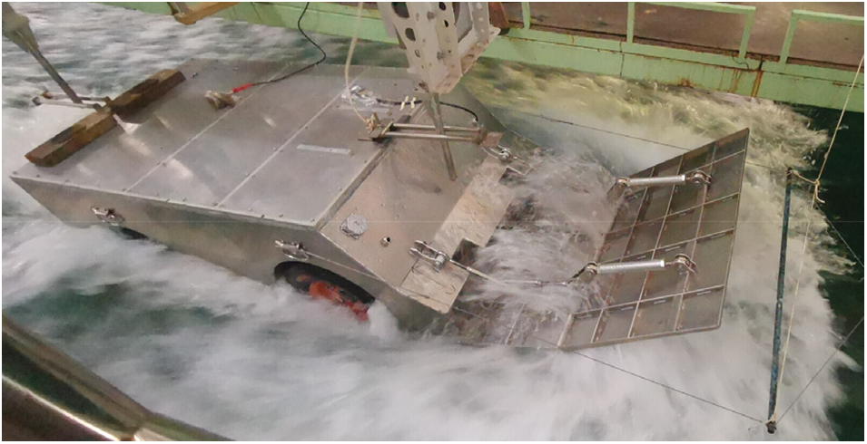
Figure 5: Towing test of amphibious unmanned vehicle

Based on the current numerical calculation model, the resistance of the amphibious unmanned vehicle at five speeds, 3.6, 5.4, 7.2, 9, and 10.8 km/h, was simulated using the STAR-CCM+, and compared with the data from the towing test. The comparison results are shown in Fig. 6.

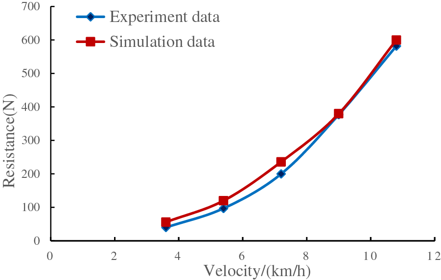
Figure 6: Comparison of numerical calculation and experimental data

It can be concluded that the numerical error of resistance at low speed is larger than that at high speed and the maximum error is 12%. With the increase in speed, the accuracy is stable at more than 94%, and the minimum error of simulation is less than 3%. The resistance variation trend of numerical calculation is consistent with the towing test, and the results of numerical calculation are consistent with those of the towing test. Considering the obvious wave-generating effect caused by the blunt bow of the amphibious unmanned vehicle, and the simplification of structures such as wheels, anti-wave plate links, and water jet in the modeling process, the calculation error is within a reasonable range, the numerical simulation results are credible, and the numerical model can be used for the numerical simulation of amphibious unmanned vehicle.

In summary, the numerical computational model of an amphibious unmanned vehicle has been established by using the VOF method and the overlapping grid technique. The independence of the time step and the number of grids were verified, and the numerical resistance values at different speeds were compared with the results of the towing test to verify the validity of the numerical model. Based on this numerical model, the following section will analyze the effect of the center of gravity position of the unmanned vehicle on the navigation characteristics and the effect of the combination of the angle of the anti-wave plate and the center of gravity position on the resistance characteristics by using the orthogonal experimental method.

3.2 Influence of the Position of the Center of Gravity on the Results of Resistance

The center of gravity of the amphibious vehicle is adjusted by moving the 48 v battery pack, which is fixed to the chassis rail. The angle between the upper anti-wave plate and the ground is 30°, and the lower is 12°. Using the above numerical model and related settings, the position of the center of gravity of the amphibious unmanned vehicle was changed to simulate, the resistance and navigation attitude of the center of gravity of the unmanned vehicle at three different positions were compared when the driving speed was 2 m/s. The calculation results of resistance are shown in Table 3.

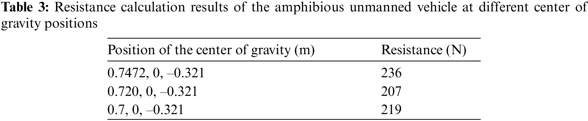
It can be seen from Table 3 and Fig. 7 that the different center of gravity positions of the amphibious unmanned vehicle have little influence on the waveform of the free surface around the vehicle at low speed. When the center of gravity is shifted backward along the x-direction of the amphibious unmanned vehicle to the position of 0.720 m, the trim angle increases and the wet area of the vehicle decreases at the same time as the bow wave decreases, which leads to a decrease in the value of the resistance.

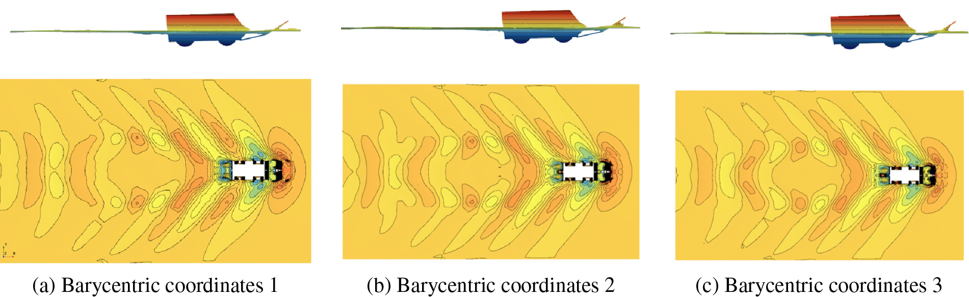
Figure 7: Navigation attitude and flow field of the amphibious unmanned vehicle with different center of gravity positions

When the center of gravity is shifted backward to the position of 0.7 m, the trim angle of the vehicle continues to become larger, and the increase of the rear sinking leads to a further increase in the shape resistance so that the navigation resistance increases again when the center of gravity continues to shift back. Because of this, a reasonable center of gravity position is of great significance for the resistance reduction characteristics of the amphibious unmanned vehicle.

4  Multi Parameter Optimization Based on Orthogonal Experimental Method

4.1 Orthogonal Experimental Design

Orthogonal experiment is an experimental design method used to study multi-factor and multi-level experiments. The researcher can choose the appropriate orthogonal table according to the number of factors and the number of levels of the factors in the experiment and use the orthogonal table to arrange the test combination scientifically according to the requirements, avoiding the huge workload due to the combination between multiple variables and obtaining the appropriate results through the fewer number of experiments.

For the optimization design of 3 factors and 3 levels in this example, if the combinations are carried out according to the traditional mathematical method, all the 3 levels of the 3 factors will be tested, and it is necessary to calculate 27 times, which is a large number of calculations and low efficiency. By applying orthogonal experimental design and using the L9(34) orthogonal table to arrange the experiments, the number of experiments can be reduced to 9 times, which improves the efficiency of the experiments.

The anti-wave plate is a segmented structure, which is divided into upper and lower plates, as shown in Fig. 8. According to the actual driving attitude of the amphibious unmanned vehicle and related test conditions, to avoid the phenomenon of burying the head when sailing, the minimum angle of the upper plate was set to 18° and the maximum to 32°, the minimum angle of the lower was set to 9° and the maximum to 15°. The center of gravity was changed along the x-axis of the driving direction, and the x-axis coordinate of the maximum value (the center of gravity is in the forward direction) was 747.2 mm. The numerical simulation speed was set at 2 m/s.

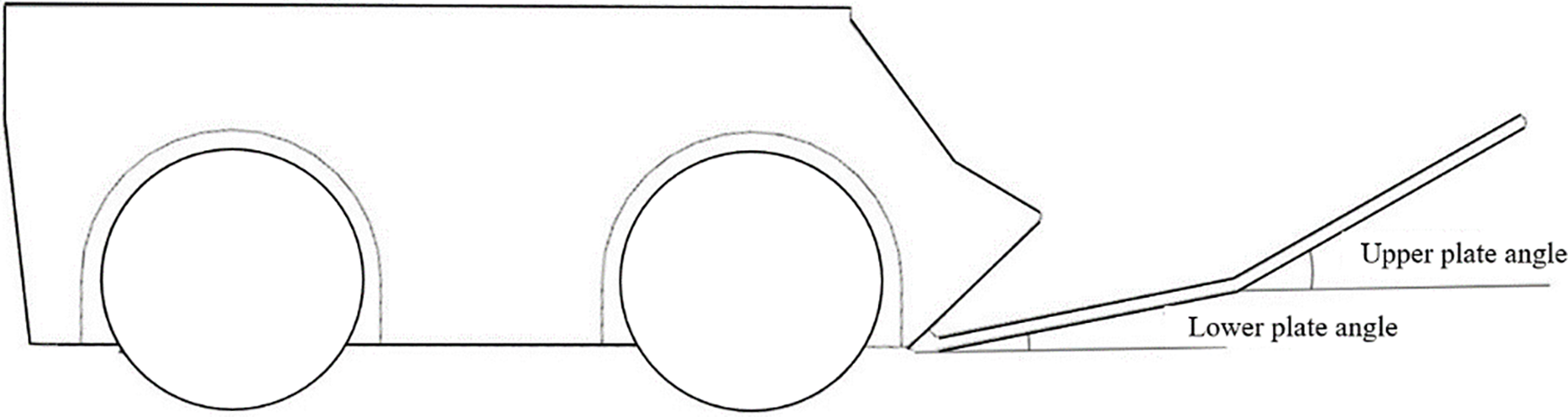
Figure 8: Angle of the anti-wave plate

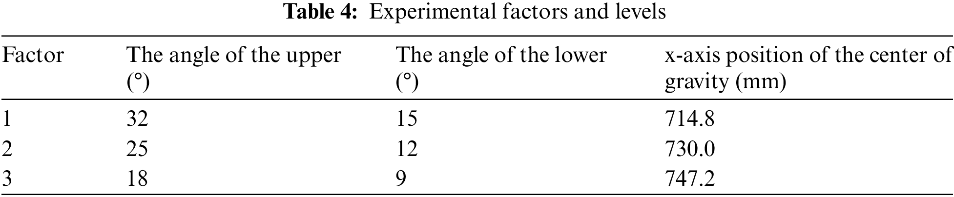
The three factors of the orthogonal experiment and the levels of corresponding factors are shown in Table 4. Among them, the numerical model settings, meshing methods, and boundary conditions are consistent for different parameter levels of each factor.

4.2 Results of the Orthogonal Experiment and Analysis

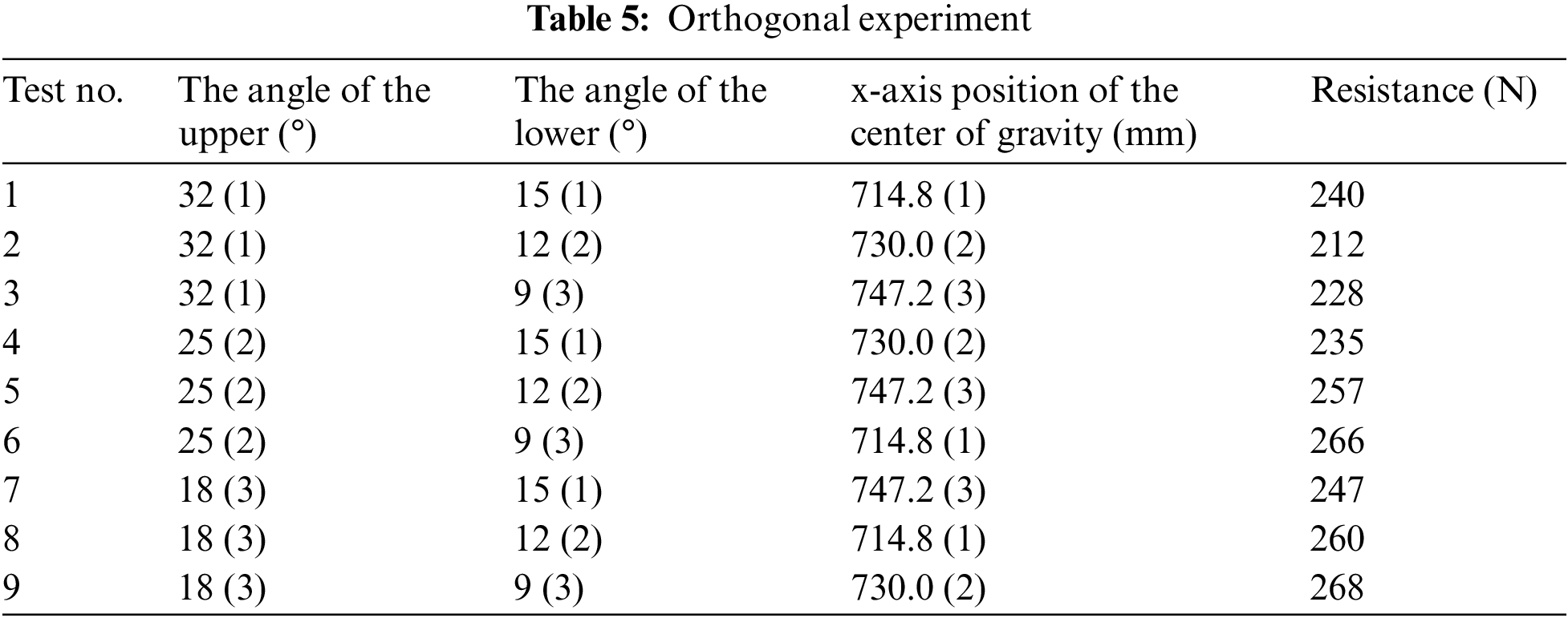
The three-dimensional model was modified according to the test scheme designed by the orthogonal table, and the simulation numerical model was re-established for numerical calculation and the results of resistance calculations are shown in Table 5.

After the completion of the numerical calculation based on the orthogonal experiment, the range analysis was carried out on the calculation results to analyze the influence of various factors on the results and find the optimal solution, that is, the factor level combination of the minimum navigation resistance and the main factor affecting the experiment results. The analysis results are shown in Table 6 and Fig. 9.

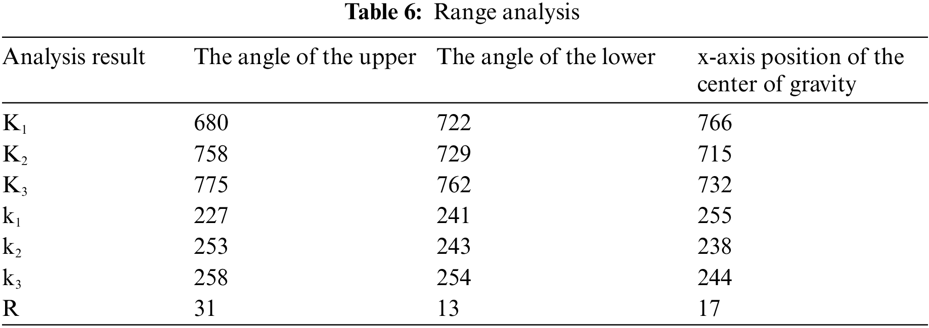
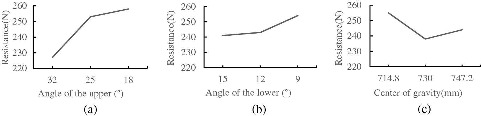
Figure 9: Intuitive analysis of the index chart

In Table 6, the K value is the sum of the results of 3 levels corresponding to experiment factors in each column of orthogonal tables. For example, K1 = 240 + 212 + 228 = 680. k is the average value of K. For example, k1 = 680/3 = 227. R is the range of the mean.

The analysis revealed that the orthogonal experimental method obtained conclusions with a smaller number of experiments. It can be seen from Fig. 9 and Table 6 that the range of each factor is different, indicating that the changes of different factors have different effects on the experiment results, and the greater the range difference, the more significant the effect is. The influence of the angle of the upper plate on the navigation resistance is more obvious than that of the angle of the lower plate and the center of gravity. Although the change of the center of gravity changes the trim angle of the vehicle, the influence of the center of gravity on the resistance becomes small when the experiment is combined with other factors. The optimal solution of resistance, i.e., the minimum value of resistance, is obtained when the test level is A1B1C2, i.e., when the angle of the upper plate is 32°, the lower plate is 15°, and the x-axis position of the center of gravity is located at 730 mm.

4.3 Orthogonal Analysis Optimal Solution Verification

For the parameter combination of experiment level A1B1C2, the model was established for simulation verification. The numerical simulation results are shown in Figs. 10 and 11. The resistance was calculated to be 203 N, which conformed to the optimal parameter combination predicted by the orthogonal experiment.

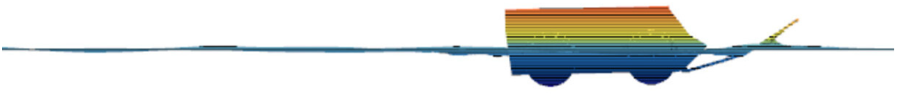
Figure 10: The driving posture of the amphibious unmanned vehicle under optimal parameter combination

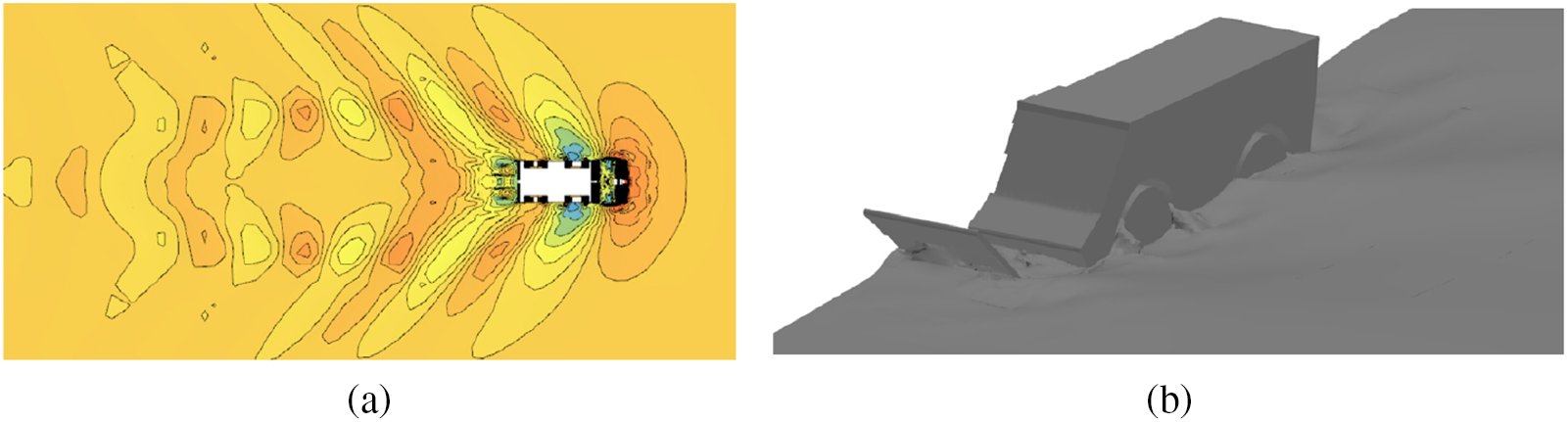
Figure 11: Flow field around the amphibious unmanned vehicle under optimal parameter combination

As can be seen from the flow field around the unmanned vehicle, the driving posture of the unmanned vehicle at this time is similar to that of a ship, with a crest appearing at the head of the vehicle and a trough appearing at the tail. The wheels of the vehicle cause a sudden change in the shape of the underside, and the flow separation phenomenon occurs when water flows through, the flow rate decreases and low-pressure areas form on both sides of the wheel, increasing the pressure difference resistance during navigation, at the same time, due to the lower pressure on both sides of the front wheels, large trough appears near the sides of the wheels, and the wave-generating effect also leads to the increase of resistance. In the subsequent optimization study of the amphibious unmanned vehicle, the wheels of the vehicle need to be considered to further reduce the navigation resistance and optimize the flow field around the amphibious unmanned vehicle.

5  Conclusions

In this paper, the navigation characteristics of the amphibious unmanned vehicle in static water were simulated by a numerical computation method, and a drag-reducing optimization method for amphibious vehicles was proposed. The parameter optimization analysis on the angle of the anti-wave plate and the position of the center of gravity was carried out by using the orthogonal test method. The main conclusions are as follows:

(1) Numerical calculations of resistance were carried out for the amphibious unmanned vehicle at different speeds, and the results of the numerical calculation were compared with the results of the towing test, which proved the effectiveness of the numerical simulation of the unmanned amphibious vehicle. When navigating in still water, the shift of the position of the vehicle’s center of gravity changes the trim angle, thus affecting the resistance characteristics of the vehicle. The research shows that the navigation resistance will decrease within a certain range when the center of gravity is shifted back to a certain position. However, as the center of gravity continues to move backward, because of the increase of the trim angle resulting in a change in the composition of resistance, navigation resistance will increase.

(2) The orthogonal experimental method was used to arrange the experiment for the combinations of the angle of the upper and lower anti-wave plate and the position of the vehicle’s center of gravity. The resistance data of different combinations were obtained by numerical calculation, and the results were reasonably analyzed using the range analysis method to predict the optimal solution and verify the validity of the prediction by numerical computation. Compared with the maximum resistance (268 N), the resistance of the amphibious unmanned vehicle is reduced by 24% and compared with the simulation result (236 N) of the amphibious vehicle under the same conditions as the parameters of the towing experiment, the resistance of the optimal solution is reduced by 14%, when the angle of the upper plate is 32°, the angle of the lower plate is 15°, and the x-axis center of gravity position is 730 mm. It can be seen that the application of the orthogonal experimental method to the multi-parameter optimization of amphibious vehicles proposed in this paper has significant results.

Acknowledgement: We would like to acknowledge that this work would not have been possible without the support of China University of Mining and Technology (Beijing) Institute of Intelligent Mining & Robotics and we sincerely thank the editors and reviewers for their review and recommendations.

Funding Statement: This work was supported by the National Natural Science Foundation of China (52174154).

Author Contributions: The authors confirm contribution to the paper as follows: study conception and design: Deyong Shang, Yanqi Niu; field experiment: Deyong Shang, Xi Zhang, Hang Yang; data collection: Xi Zhang, Fengqi Liang; analysis and interpretation of results: Xi Zhang, Chunde Zhai; draft manuscript preparation: Hang Yang. All authors reviewed the results and approved the final version of the manuscript.

Availability of Data and Materials: The field towing data is publicly available, while the research work is based on computer numerical simulation with a huge amount of simulation data. Due to the continuation of subsequent optimization work, some data may not be publicly available. For those interested in this study, please contact the author of the paper for further information and access to the relevant data.

Conflicts of Interest: The authors declare that they have no conflicts of interest to report regarding the present study.

References

1. Sun, C. L., Xu, X. J., Wang, W. H., Xu, H. J. (2020). Influence on stern flaps in resistance performance of a caterpillar track amphibious vehicle. IEEE Access, 8, 123828–123840. https://doi.org/10.1109/ACCESS.2020.2993372 [Google Scholar] [CrossRef]

2. Nakisa, M., Maimun, A., Ahmed, Y. M., Behrouzi, F., Tarmizi, A. (2014). RANS simulation of viscous flow around hull of multipurpose amphibious vehicle. International Journal of Mechanical and Mechatronics Engineering, 8, 298–302. [Google Scholar]

3. Pan, D. B., Xu, X. J., Liu, B. L. (2021). Influence of flanks on resistance performance of high-speed amphibious vehicle. Journal of Marine Science and Engineering, 9(11), 1260. https://doi.org/10.3390/jmse9111260 [Google Scholar] [CrossRef]

4. Behara, S., Arnold, A., Martin, J. E., Harwood, C. M., Carrica, P. M. (2020). Experimental and computational study of operation of an amphibious craft in calm water. Ocean Engineering, 209, 107460. https://doi.org/10.1016/j.oceaneng.2020.107460 [Google Scholar] [CrossRef]

5. Su, Y. M., Wang, S., Shen, H. L., Du, X. (2014). Numerical and experimental analyses of hydrodynamic performance of a channel type planing trimaran. Journal of Hydrodynamics, 26, 549–557. https://doi.org/10.1016/S1001-6058(14)60062-7 [Google Scholar] [CrossRef]

6. More, R. R., Adhav, P., Senthilkumar, K., Trikande, M. W. (2014). Stability and drag analysis of wheeled amphibious vehicle using CFD and model testing techniques. Applied Mechanics and Materials, 592–594, 1210–1219. https://doi.org/10.4028/www.scientific.net/AMM.592-594.1210 [Google Scholar] [CrossRef]

7. Xu, H. J., Xu, L. Y., Feng, Y. K., Xu, X. J., Jiang, Y. et al. (2023). Influence of a walking mechanism on the hydrodynamic performance of a high-speed wheeled amphibious vehicle. Mechanical Sciences, 14(2), 277–292. https://doi.org/10.5194/ms-14-277-2023 [Google Scholar] [CrossRef]

8. Demirel, Y. K., Khorasanchi, M., Turan, O., Incecik, A., Schultz, M. P. (2014). A CFD model for the frictional resistance prediction of antifouling coatings. Ocean Engineering, 89, 21–31. https://doi.org/10.1016/j.oceaneng.2014.07.017 [Google Scholar] [CrossRef]

9. Yang, X. F., Yan, X., Liu, W., Ye, H., Du, Z. P. et al. (2022). An improved stanley guidance law for large curvature path following of unmanned surface vehicle. Ocean Engineering, 266, 112797. https://doi.org/10.1016/j.oceaneng.2022.112797 [Google Scholar] [CrossRef]

10. Ma, D. F., Hao, S. F., Ma, W. H., Zheng, H. R., Xu, X. L. (2022). An optimal control-based path planning method for unmanned surface vehicles in complex environments. Ocean Engineering, 245, 110532. https://doi.org/10.1016/j.oceaneng.2022.110532 [Google Scholar] [CrossRef]

11. Yang, X. F., Shi, Y. L., Liu, W., Ye, H., Zhong, W. B. et al. (2022). Global path planning algorithm based on double DQN for multi-tasks amphibious unmanned surface vehicle. Ocean Engineering, 266, 112809. https://doi.org/10.1016/j.oceaneng.2022.112809 [Google Scholar] [CrossRef]

12. Jang, J. Y., Liu, T. L., Pan, K. C., Chu, T. W. (2019). Numerical investigation on the hydrodynamic performance of amphibious wheeled armored vehicles. Journal of the Chinese Institute of Engineers, 42, 700–711. https://doi.org/10.1080/02533839.2019.1660225 [Google Scholar] [CrossRef]

13. Dhana, F. R., Park, J. C., Yoon, H. K. (2023). A numerical study on the influence of caterpillars to the resistance performance of an amphibious vehicle. Journal of Marine Science and Engineering, 11, 286. https://doi.org/10.3390/jmse11020286 [Google Scholar] [CrossRef]

14. Luo, H., Ding, J. M., Jiang, J. B., Li, L. X., Gong, J. et al. (2022). Resistance characteristics and improvement of a pump-jet propelled wheeled amphibious vehicle. Journal of Marine Science and Engineering, 10, 1092. https://doi.org/10.3390/jmse10081092 [Google Scholar] [CrossRef]

15. Helvacioglu, S., Helvacioglu, I. H., Tuncer, B. (2011). Improving the river crossing capability of an amphibious vehicle. Ocean Engineering, 38(17–18), 2201–2207. https://doi.org/10.1016/j.oceaneng.2011.10.001 [Google Scholar] [CrossRef]

16. Latorre, R., Arana, J. (2011). Reduction of amphibious vehicle resistance and bow swamping by fitting a wave cancellation bow plate. Naval Engineers Journal, 123(4), 81–89. https://doi.org/10.1111/j.1559-3584.2010.00265.x [Google Scholar] [CrossRef]

17. Tolstonogov, A. Y., Dzyaman, M. A., Sebto, A. Y., Filonov, I. V., Chemezov, I. A. (2019). The compact ROV with variable center of gravity and its control. 2019 IEEE Underwater Technology (UT), pp. 1–7. Kaohsiung, Taiwan. [Google Scholar]

18. Hirt, C. W., Nichols, B. D. (1981). Volume of fluid (VOF) method for the dynamics of free boundaries. Journal of Computational Physics, 39(1), 201–225. [Google Scholar]

19. Ren, Z., Wang, J. H., Wan, D. C. (2020). Investigation of the flow field of a ship in planar motion mechanism tests by the vortex identification method. Journal of Marine Science and Engineering, 8(9), 649. https://doi.org/10.3390/jmse8090649 [Google Scholar] [CrossRef]

20. JI, S. C., Ouahsine, A., Smaoui, H. (2012). 3D numerical simulation of convoy-generated waves in a restricted waterway. Journal of Hydrodynamics, 24(3), 420–429. [Google Scholar]

21. Wang, T., Xu, G. Y., Yao, X. M., Zhou, J. T. (2008). Numerical simulation of two phases flow field around amphibious vehicle and analysis of power performance on water. Chinese Journal of Mechanical Engineering, 44(12), 168–172. https://doi.org/10.3901/JME.2008.12.168 [Google Scholar] [CrossRef]

22. Wang, J. H., Wan, D. C. (2020). CFD study of ship stopping maneuver by overset grid technique. Ocean Engineering, 197, 106895. https://doi.org/10.1016/j.oceaneng.2019.106895 [Google Scholar] [CrossRef]

23. Kunihide, O., Hiroshi, K., Takanori, H. (2018). Numerical simulation of the free-running of a ship using the propeller model and dynamic overset grid method. Ship Technology Research, 65(3), 153–162. https://doi.org/10.1080/09377255.2018.1482610 [Google Scholar] [CrossRef]