Gyroscope Dynamic Balance Counterweight Prediction Based on Multi-Head ResGAT Networks

Nomenclature

1  Introduction

The dynamic balance performance of a gyroscope within a dynamic-gyro coordinator profoundly influences its precision in guidance [1]. In a rotating 3-DOF (3 Degrees of Freedom) gyroscope, dynamic balance over-proof results in unbalanced forces. This occurs when the barycenter deviates from the rotation axis, leading to mechanical vibration, compromised connection reliability, reduced bearing lifespan, and diminished positioning accuracy [2]. With high performance precision requirement and complex process, the manual assembling and debugging in the gyroscope production can prove inefficient when the dynamic balance capability is unstable.

As seen in Fig. 1, in the assembling process of gyroscope, the debugging of dynamic balance utilizes counterweights attached to the front and rear counterbalance-surfaces separately.

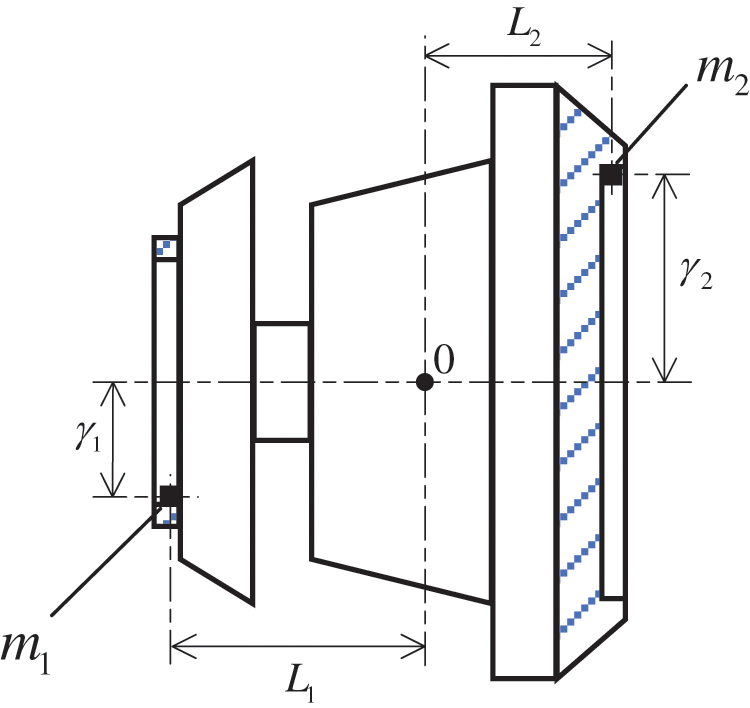
Figure 1: The gyroscope dynamic balance debugging

To counteract the unbalanced forces, the centrifugal forces produced by two counter weight-blocks should be kept in the direction opposite to the resultant unbalanced force [3], as shown in Eq. (1):

m1γ1ω2+m2γ2ω2=KR(1)

where m1 and m2 are the counterweights. γ1 and γ2 are the rotation radiuses, R is the resultant unbalanced force, and K is the sensitivity coefficient of dynamic balancing instruments;

Meanwhile, the moments produced by m1 and m2 should counteract each other to keep the balance:

m1γ1L1=m2γ2L2(2)

where L1 and L2 are the axial distances between barycenter and counterweight-blocks.

Thus, in the assembling process of gyroscope, empirical formulas are summarized from production experience to calculate the counterweights:

m1=k1G(3)

m2=k2G(4)

where G is the initial dynamic balance figure measured by instruments and should be proportional to the counterweights theoretically, k1 and k2 are the counterweight-coefficients.

In this paper, we regard the rear counterweight m2 as the counterweight figure we research on while the front counterweight m1 is determined by m2 in engineering design.

Empirical formulas may exhibit suboptimal performance in dynamic balance debugging, attributed to unquantifiable machining errors in components and manual assembly-induced assembling errors. Fig. 2 illustrates substantial disparities between counterweights determined by empirical formulas and those mandated by the actual dynamic balance requirements of the gyroscope.

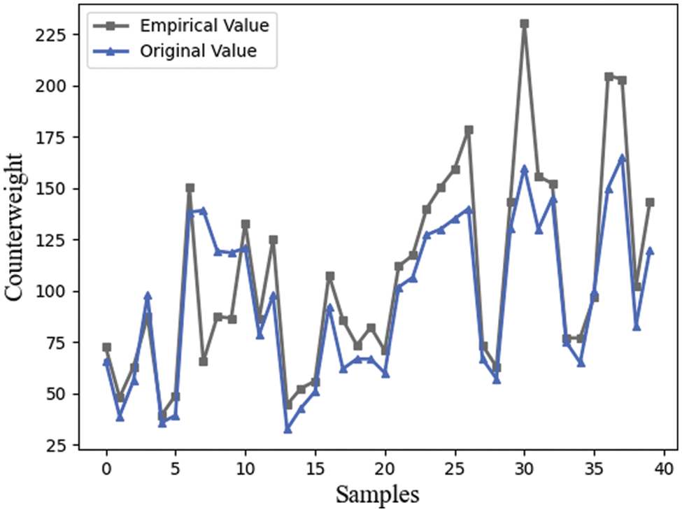
Figure 2: Calculated counterbalance and the real counterbalance required

Inaccurate counterweights leading to poor dynamic balance performance necessitate repetitive assembly and disassembly of counterweight-blocks, gimbals, and flanges. This results in inefficiencies and errors in manual assembly processes [3]. Our research on various gyroscope types indicates that inaccurate counterweight predictions from empirical formulas elevate the assembly repetition rate by more than 50%, consequently escalating man-hours and production costs. Thus, there is a critical need for more precise counterweight predictions to enhance the one-time fitting acceptance rate and improve gyroscope productivity.

To obtain more accurate counterweights, an analysis of factors underlying the dynamic balance capability of gyroscopes is essential. Due to the intricate structure of gyroscopes, constructing a precise physical model is impractical [4]. However, based on engineering experiences, assembly parameters of gyroscope components have been identified as potentially relevant to the required counterweights and can be examined through association analysis. The results of linear correlation analysis between assembly parameters and counterweights are presented in Table 1.

Where R is the coefficient of determination (Pearson coefficient), which is the square of multiple correlation coefficient. Generally, linear fitting results better when R is closed to 1 [5].

As indicated in Table 1, the assembly parameters exhibit negligible linear correlations with the counterweight [6]. This implies that there may exist nonlinear couplings between these variables, rendering it impractical to establish functional relationships solely based on dynamic theories. Moreover, traditional feature selection techniques such as principal component analysis (PCA) and linear discriminant analysis (LDA) may no longer be appropriate for association analysis, given the absence of significant linear correlations.

Multivariate Analysis of Variance (MANOVA) is a statistical method employed for association analysis, evaluating the significance of associations through variance comparisons and hypothesis testing [7]. MANOVA is suitable for data with nonlinear couplings, as it examines the overall variation of the counterweight concerning assembly parameter variations. Additionally, MANOVA accounts for potential interactions between different parameters, even when their relevance is not explicitly established [8]. The concurrent probability (P), derived from the F distribution table, is compared to the level of significance (α). If P ≤ α, it signifies a significant impact of assembly parameter variation on the counterweight; otherwise, the parameter is deemed irrelevant [9]. Results of MANOVA are presented in Table 2.

Where Interaction 1 is the interaction between flange edge height and bearing clearance, Interaction 2 is the interaction between bearing clearance and curing coaxiality, and Interaction 3 is the interaction between flange edge height and curing coaxiality.

As shown in Table 2, the parameters which have significant impact are flange edge height, bearing clearance, and curing coaxiality. Meanwhile, Interaction 1 and Interaction 2 also badly affect the counterweight of gyroscope.

In summary, in the acquisition of accurate gyroscope counterweight, the following problems exist:

1. The empirical formulas commonly used for counterweight calculation in the complex system of gyroscope assembly have been found to be inaccurate due to the potential assembly deviation. Dynamic theory has been found to be inadequate in establishing accurate functional relations in this context.

2. Deep neural networks have gained widespread popularity in nonlinear analysis and performance prediction [10]. In particular, a deep neural network may be employed to model the intricate relationships between assembly parameters and counterweight. However, due to limited availability of historical assembly data resulting from small batch production of dynamic gyroscopes, the size of the training set may lead to under-fitting results when using traditional neural network models.

3. Interactions among assembly parameters in gyroscope assembly are influenced by unquantifiable factors such as manual operating errors and fitting errors between gyroscope components. Analysis reveals that parameter interactions significantly impact the counterweight, with the association’s significance varying with the gyroscope assembly sequence, as detailed in Section 4.2. These complexities in interactions can lead to poor learning effects and low fitting accuracy in the model.

In recent decades, numerous studies have been conducted on dynamic gyroscope performance analysis and compensation, with many utilizing dynamic modeling and simulation. One related work was proposed by Fang et al. [11], which employed a non-dimensional time-position dynamic model for the performance analysis of micro electro mechanical system (MEMS) gyroscope. The model was capable of simulating gyroscope trajectory and estimating parameters. Tu et al. presented an applying autoregressive moving average (ARMA)-based digital twin for gyroscope dynamic modeling and drift compensation [4]. Luo et al. revealed the nonlinear dynamics of gyroscope, reconstructed trajectories, and derived dynamical equations [12]. However, these methods are limited to MEMS gyroscope, the dynamic balance of which are not significantly affected by the vibration from manufacturing and assembly errors, and are therefore not applicable to complex system analysis in dynamic gyroscope assembly. Xu et al. employed prior knowledge of gyroscope multibody dynamics and support vector regression (SVR) to forecast the drift performance of dynamic gyroscopes [13]. Nonetheless, the proposed dynamic model simplified the gyroscope to a sphere, neglecting the impact of assembling and manufacturing errors. Such oversimplification may lead to significant prediction deviations in the context of gyroscope assembly. Another supervised learning method for gyroscope performance prediction was introduced by Zhang et al., who combined gyroscope estimation model with radial basis function (RBF) neural network to improve the approximation accuracy of the compound nonlinearity [14]. Meanwhile, Cao et al. presented a neural network model combined with time-frequency peak filtering (TFPF) and mind evolutionary algorithm (MEA) to predict the gyroscope drift compensation [15]. These traditional methodologies are categorized in Table 3.

Although neural-network-based models are capable of achieving high-precision compensation, they require e a large amount of training data due to the limited feature extraction ability of traditional neural networks. This renders them unsuitable for the small sample size condition of gyroscope counterweight prediction. Insufficient training data can cause neural network models to perform poorly in terms of feature extraction, leading to overfitting or under-fitting, which is commonly known as the few-shot learning problem. Meanwhile, it has been demonstrated in academic literature that the self-attention mechanism can significantly improve the ability to extract important features by adjusting the weights of inputs in each layer of the model [16]. Despite the potential use of self-attention mechanisms to tackle small-sample conditions in constrained training sets, it is crucial to acknowledge that self-attention-based models, such as transformers, exhibit a similar structure where all inputs are treated as relatively independent. This structure can result in suboptimal learning of interactions among input parameters, especially with limited-sized datasets, thereby compromising the model’s robustness.

Furthermore, graph neural networks (GNN) have been proposed as a promising alternative to traditional neural networks for modeling relevance between nodes, as they are capable of capturing both the property and interaction features of input parameters [17]. For instance, a recent study by Hong and colleagues applied a graph neural network model to learn patterns of relations from materials properties and chemical structural data and demonstrated high prediction accuracy in the context of melting temperature [18]. However, this model employed an integrated architecture of 30 graph and residual neural networks, and was trained on a database consisting of approximately 10,000 compounds. Therefore, the GNN model proposed in this study with massive weights requires a large quantity of training samples, making it infeasible for the small sample condition associated with counterweight prediction. Velickovic et al. proposed graph attention networks (GAT) by combining graph neural network with self-attention mechanism, which can efficiently process arbitrarily structured graphs [19]. Despite its success in various graph-related tasks, GAT may still suffer from the overfitting issue due to the duplicated structure and weights of small-sample assembly graph data, thus limiting the model’s ability to fit the data. Moreover, in-time graph structural data, such as the adjacency matrix of the parameters is needed when the model is adapted to gyroscope counterweight prediction. In practical gyroscope assembly production, gyroscopes are assembled and debugged in small batches, typically numbering no more than 20. Deriving accurate adjacency matrices through correlation analysis on such limited assembly data batches is not feasible.

To tackle these problems, the contribution of this paper is described as below:

1. A data-driven method for gyroscope dynamic balance counterweight prediction is proposed, which enables latent feature extraction from assembly parameter data in the nonlinear complex system of gyroscope assembly. Our method demonstrates exceptional precision at 95.68% and an assembly repetition rate as low as 5%, surpassing all existing literature methods. These results signify substantial enhancements in production efficiency.

2. To support counterweight prediction with parameter interaction information in situations where accurate association analysis is challenging with small-batch gyroscope samples, we introduce a modified model combining stacked denoising autoencoder and Gaussian process classifier (SDAE-GPC) for assembly condition classification. This model provides assembly parameter data with interaction features based on assembly conditions for the subsequent counterweight regression model.

3. To mitigate fitting inaccuracies resulting from variable interactions among assembly parameters in gyroscope assembly, we introduce a Multi-head Residual Graph Attention Network (ResGAT) model. This model integrates residual connections into graph attention networks and adjusts attention scores to enhance fitting effectiveness under small-sample conditions. Leveraging the assembly condition matrices from the SDAE-GPC model, our ResGAT model achieves heightened learning efficiency with limited weights and more precise counterweight regression.

The remainder of the paper is structured as follows:

In Section 2, we design a graph data structure to represent discrete assembly sequence data. Section 3 introduces the SDAE-GPC model for assembly condition classification to provide graph data support for counterweight prediction. The proposed ResGAT counterweight regression model utilizes condition matrices, achieving higher regression accuracy. Section 4 presents controlled experiments on assembly condition classification and counterweight regression models using practical gyroscope assembly production data, demonstrating the effectiveness and superiority of the proposed methods. Finally, in Section 5, we draw conclusions based on the research findings, emphasizing the significance of our approach in gyroscope dynamic balance counterweight prediction and discussing potential avenues for future research in this area.

2  Graph Data Structure for Assembly Condition

In assembly processes, we observe a significant influence of the gyroscope counterweight due to interactions among assembly parameters. The strength of these interactions, as determined by MANOVA analysis, varies with specific assembly sequences (detailed in 4.2).

Acknowledging the impactful variable and its potential interference in the modeling process, we propose leveraging association status information between interactions and counterweight as an input for the model. To facilitate this, we introduce a novel data structure for assembly parameter inputs, designed to precisely capture the impact of interactions and enhance predictive performance.

The utilization of graph data in the analysis of assembly processes, as suggested by Kipf and Welling, proves beneficial. Graph data effectively encodes information in a structured and meaningful manner, representing both properties and relationships between parameters [20].

Fig. 3 depicts an attributed relational graph that represents partial assembly parameters, where changes in interactions can be interpreted as changes in relationships between nodes.

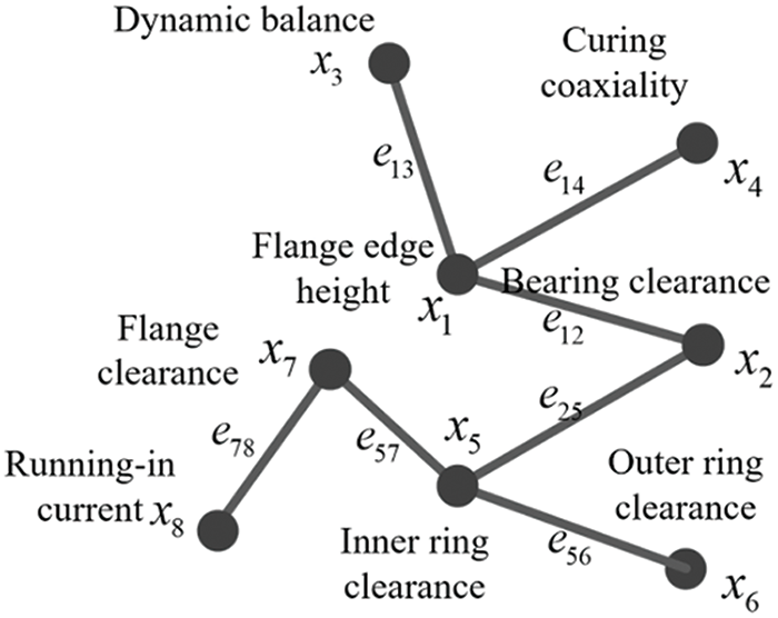
Figure 3: Attributed relational graph of partial assembly parameters

The nodes correspond to assembly parameters while the edges indicate the interactions among these parameters. The assembly parameter dataset X={X1,X2,…,Xn} is presented in the form of a property matrix XP×N, wherein the individual elements signify the attribute values associated with each node. P denotes the parameters in assembly sequences of N gyroscope samples. Adjacency matrix is utilized to represent the interaction relationships between parameters. As shown in formulas (3) and (4), the element Aij represents the existence of significant interactions. When Aij=1, the interaction of assembly parameter Xi and Xj shows strong impact on the counterweight.

A=[0A12A13⋯A1nA210A23⋯A2nA31A320⋯A3n⋮⋮⋮⋱⋮An1An2An3⋯0](5)

Aij={0,SigAB≥0.051,SigAB<0.05(6)

where SigAB denotes the concomitant probability of interaction between Xi and Xj on the counterweight in MANOVA. The interaction is considered significant when SigAB≤0.05. Meanwhile, to prevent nodes property information loss, we employ a self-loop mechanism for the adjacency matrix, as shown in formula (7).

A^=A+I(7)

where I is an identity matrix with the same shape as adjacency matrix A.

Then the adjacency matrix can be represented as A^, as shown in formula (8).

A^=[1A12A13⋯A1nA211A23⋯A2nA31A321⋯A3n⋮⋮⋮⋱⋮An1An2An3⋯1](8)

We propose an approach to represent traditional assembly data in the form of an assembly parameter graph dataset G=(A,X), which is composed of an interaction matrix A and a property X matrix. This approach provides a structural framework for training graph neural network models for generative and regression tasks.

3  Model for Counterweight Prediction

In this section, we present a novel ResGAT model adapted for few-shot gyroscope counterweight prediction. Our approach incorporates an SDAE-GPC for precise assembly condition classification, enabling accurate forecasting of gyroscope counterweight in small-batch scenarios. The entire processing diagram of the counterweight prediction method is shown in Fig. 4.

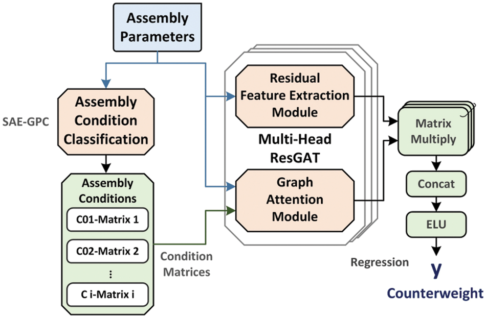
Figure 4: Processing diagram of the counterweight prediction method

As depicted in Fig. 4, the SDAE-GPC model utilizes assembly parameter features from various gyroscope production batches for pattern recognition. It furnishes the ResGAT with an assembly condition matrix, capturing the intricate interplay among parameters. Both assembly parameters and condition matrices are then fed into ResGAT for counterweight regression.

Fig. 5 illustrates the training and prediction process in our proposed model. The SDAE-GPC model is trained with labeled data and used for condition selection. In the Multi-head ResGAT model, both property and interaction features are extracted from the inputs to enhance counterweight prediction accuracy, especially in small-sample conditions.

Figure 5: Gyroscope dynamic counterweight prediction model

3.1 SDAE-GPC for Assembly Condition Classification

Stacked Denoising Autoencoder (SDAE) is an unsupervised neural network comprising multiple layers of autoencoders, each incorporating random input corruption [21]. Its architecture is akin to the stacked autoencoder (SAE), where the output of each encoder serves as input for the subsequent one, and the final encoder’s output is directed towards a sequence of decoders. This design enhances the autoencoder’s capacity for dimensionality reduction and feature extraction. Additionally, the random input corruption aids the model in developing denoising capabilities, thereby improving its accuracy in data reconstruction.

The encoding process of SDAE filters essential features from the inputs. Stacked layers of encoders extract crucial information from assembly parameter data by mapping them to low-dimensional latent vectors.

In traditional SAE architecture, a single encoder layer of can be represented as formula (9).

yl=σ(Wlx+bl)(9)

where Wl and bl are the weights and bias of layer l, and σ is activation function Sigmoid.

Meanwhile, a corruption process for the inputs is adopted for denoising ability training, where the initial input x is zeroed to a scale in stochastic mapping qD, as is shown in formula (10).

x~=qD(x~|x)(10)

where x~ is the corrupted input.

With this process, model can learn to extract features useful for denoising when reconstructing the inputs during training. The corrupted inputs are then mapped to low dimensional latent features with encoders.

The forward propagation of SDAE encoder layers can be represented as formula (11).

zl=σ(Wlx~+bl)(11)

where zl is the output latent feature of layer l.

In this paper, we adopt a stacked architecture composed of three autoencoders for dimensionality reduction. The hidden output of each encoder layer is utilized as the input of the next encoder, as shown in formulas (12) and (13).

zl−1=σ(Wl−1x~+bl−1)(12)

zl=σ(Wlz~l−1+bl)(13)

where 1≤l≤3

The decoder of SDAE attempts to achieve the reconstruction of assembly parameter graph data with the latent variables derived from the encoders, utilizing corresponding stacked layers. As is shown in formulas (14) and (15).

zl−1=σ(Wl−1′z+bl−1′)(14)

x^=σ(Wl′zl−1+bl′)(15)

where x^ is the reconstructed assembly parameter data, Wl′ and bl′ are the weights and bias of layer l, 1≤l≤3.

In small-sample training conditions, the under-fitting problem is prevalent due to data noise. To address this, we adopt a pre-training and fine-tune strategy in training the SDAE for improved denoising efficiency.

In the pre-training phase, the SDAE is trained using unlabeled assembly parameter data to acquire denoising and dimension reduction capabilities. During this process, the corruption mechanism compels the model to discern distinctions between corrupted and original inputs, enhancing its denoising capability.

The pre-training process of the SDAE-GPC condition classification model is shown in Fig. 6.

Figure 6: Pre-training process of SDAE-GPC model

As shown in Fig. 6, The encoder in the SDAE generates low-dimension latent variables that extract higher-level features from the assembly parameter data. These variables aim to capture the most important information and provide a more condensed representation of the inputs.

We adopt MSE for the loss function in pre-training, as shown in formula (16).

loss=MSE(x^,x)=‖x^−x‖2(16)

During the fine-tuning process, the model’s learned features undergo further refinement using original assembly parameter data and corresponding assembly condition labels to enhance overall performance. Fine-tuning with denoised features and initialized weights contributes to a more effective convergence.

The finetune process of SDAE is shown in Fig. 7.

Figure 7: Fine-tuning process SDAE-GPC model

The forward propagation of the fine-tuning process is shown in formulas (17) and (18).

zl−1=σ(Wl−1″x+bl−1″)(17)

zl=φ(Wl″zl−1+bl″)(18)

where zl is the output of SDAE, φ is activation function softmax, Wl″ and bl″ are the weights and bias of layer l, 1≤l≤3.

The resultant latent features are fed into a Gaussian Process Classifier (GPC) for assembly condition classification. Unlike deterministic classifiers such as logistic regression or support vector machines, GPC models the decision boundary between different classes as a probability distribution over functions, capturing both the mean and the uncertainty of predictions. This advantage renders GPC suitable for uncertain interaction feature extraction in assembly parameter data. With an unstationary kernel function like the polynomial kernel, GPC can effectively handle high-dimensional nonlinearity issues such as assembly condition classification. Hence, we employ the dot product kernel for the GPC classifier, with the kernel function depicted in formula (19).

K(x,xi)=(x⋅xi+1)d(19)

where d=1,2,…,N.

The SDAE architecture’s denoising, dimensionality reduction, and feature extraction capabilities facilitate the transformation of assembly parameter data into higher-level latent features, enhancing accuracy in classification by the subsequent classifier.

The loss function in the fine-tuning process is expressed in formula (20). Cross-Entropy function is employed to quantify the residual in assembly condition classification.

loss=CrossEntropy(y^,y)=−1N∑nylog⁡y^−(1−y)log⁡(1−y^)(20)

where y is the output of SDAE-GPC assembly condition classification model, y^ is the actual condition label of the corresponding assembly parameter, N is the number of gyroscopes in an assembly sequence when calculating the residual of each epoch of training.

The model becomes proficient in predicting the gyroscope assembly condition based on the assembly parameters. Consequently, we acquire the corresponding adjacency matrix for each assembly condition, serving as the input for training the ResGAT counterweight prediction model proposed in this study.

3.2 Residual Graph Attention Network for Counterweight Regression

GAT operates on graph data and extracts property and relation features of nodes with hidden masked self-attentional layers [20], leveraging attention mechanisms to handle variable inputs and focus on the most relevant parts. Assembly parameter graph data can be processed by graph attention architectures for the acquisition of higher-level features. Furthermore, to address the overfitting problem under small-sample condition, residual net structures are brought to graph attention mechanism to enable skip connects in the calculation of attention coeficient and the forward propagation of the model.

As shown in Fig. 8, the ResGAT network is constructed with residual feature extraction modules and graph attention modules. Essential property features from the assembly parameter data are expressed through layers with residual connection. Meanwhile, the attention module provides learning focus based on the interaction information of the parameters, which allows the nodes to attend over their neighborhoods’ features.

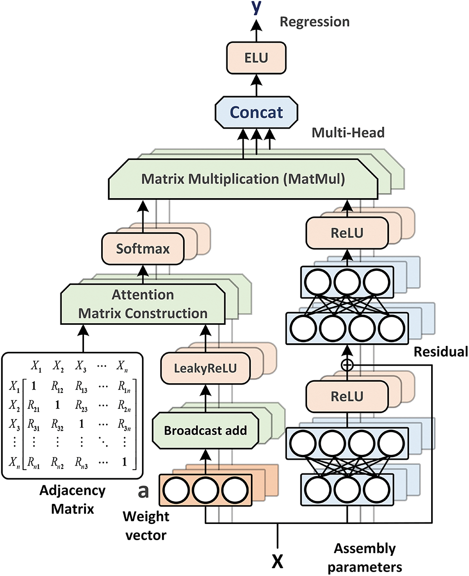
Figure 8: Multi-head ResGAT counterweight prediction model

The inputs of our model include the normalized assembly parameter data X={x1,x2,…,xn} and the corresponding adjacency matrix A={A1,A2,…,Am} from different assembly condition, as described in Section 2, where n is the number of parameter nodes and m is the number of assembly conditions.

In attention modules, assembly parameters are firstly utilized for the calculation of attention coefficient e. In this paper, we modified the definition of the attention coefficient to control the weight quantity of the model, as shown in formula (21).

e=leakyReLU((x×a)+(x×a)T)(21)

where x is the assembly parameter inputs, a is the trainable attention weight, and leakyReLU is the activation function shown in formula (22). The plus sign here stands for the broadcast add of matrices.

y=max(0,x)+leak⋅min(0,x)(22)

where leak is an adjustable constant ensuring the negative values.

Furthermore, an attention matrix Att is constructed with the attention coeficient e and zeros, based on the adjacency matrix A, as shown in formulas (23) and (24).

attij={e,aij=10,aij=0(23)

Attij=softmax(attij)=exp⁡(attij)∑k∈Niexp⁡(eik)(24)

where aij is the element of the adjacency matrix A, Attij is the element of attention matrix Att, and Ni is the neighborhood amount of node i in the graph.

As shown in Fig. 8, residual connections are appended to the layers to avoid degradation in training and derive more accurate regression. After nonlinear transformation, the hidden variables are then multiplied with the attention matrix obtained from the attention module for the output, as shown in formula (25).

h=Att×σ(x+σ(x×w1))×w2(25)

where w1 and w2 are the weights and σ is the activation function ReLU shown in formula (26).

y=max(0,x)(26)

In this paper, we also employ multi-head architecture for the best effect of attention mechanism. Outputs of independent ResGAT network structures are concatenated and represented in formula (27), to derive the final output of the multi-head ResGAT model.

output=σ′(∥k=1Khk)(27)

where ∥ represents the concatenation process, K is the number of heads, and σ′ is the activation function CELU shown in formula (28).

CELU(x)=max(0,x)+min(0,α⋅(exp⁡(x/α)−1))(28)

where α is a hyper-parameter, in this paper α=0.9 is taken for the best training effect.

The loss function of the ResGAT model is shown in formula (29). The root mean square error (RMSE) cost is adopted to measure the residual in counterweight regression.

loss=1n∑i=1n(yi−y^)2(29)

where y and y^ are the label and prediction of the gyroscope counterweight value and n is the amounts of samples.

During training, the model incorporates attention mechanisms based on assembly graph data and residual connection structures to prevent overfitting and degradation, especially with a small-sized training set. Weighted feature aggregation is achieved through the multi-head output unit for effective regression. Consequently, the model is readily applicable to predicting gyroscope counterweights using assembly parameter graph data.

4  Experiments and Discussion

4.1 Gyroscope Assembly Data Preparation

In this study, assembly datasets were gathered from historical data of a specific type of dynamic gyroscope, encompassing assembly and debugging parameters from 1000 in-line gyroscope assembly samples. The dataset for assembly condition classification includes key parameters from prior dynamic gyroscope assembly processes, such as gimbal assembly, magnetization, and preliminary dynamic balance surveys.

Simultaneously, the dataset for counterweight prediction includes assembly parameters selected via MANOVA due to their substantial impact on the corresponding counterweights (as detailed in Section 4.2).

All training parameters were initially normalized to ensure model stability and accuracy. Normalization, as shown in formula (30), is crucial for bringing features to a common scale, facilitating balanced weighting during model initialization.

Xnorm=X−XminXmax−Xmin(30)

where X is the original parameter sample from the assembly sequences, Xmax is the maximum sample of X and Xmin is the minimum. Partial normalized parameter data is shown in Table 4.

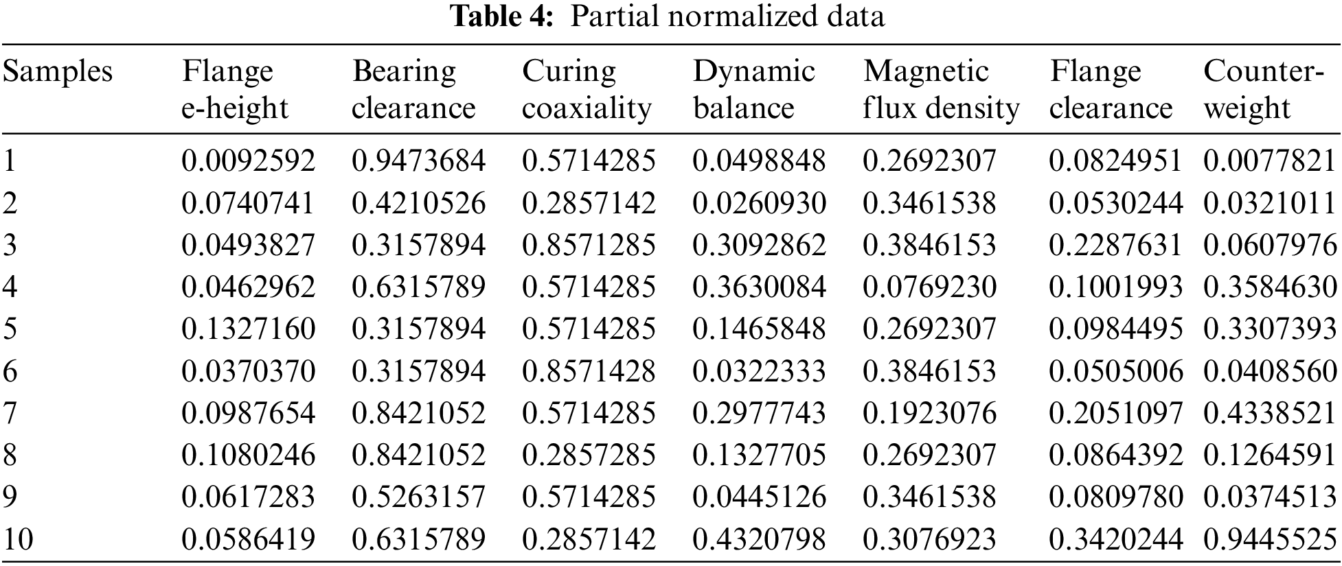
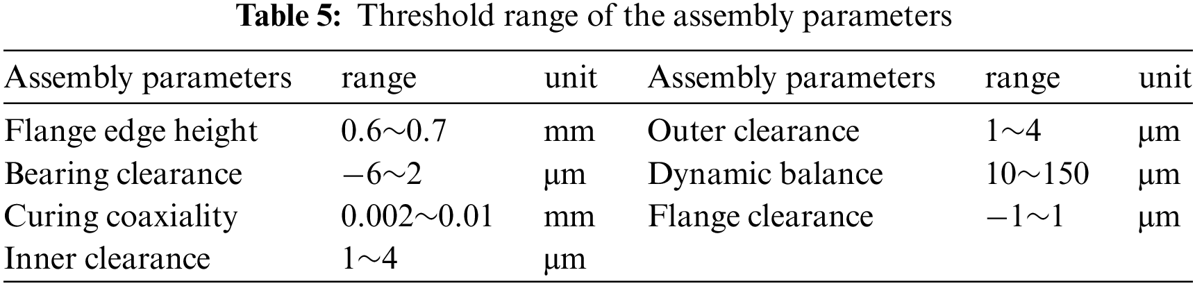
The threshold range of the assembly parameters is shown in Table 5.

The dataset was divided independently for the assembly condition classification model and the gyroscope counterweight prediction model. Both the training and test sets were split in a 4:1 ratio [22]. For the SDAE-GPC classification model, the training set encompassed parameter data for both the pre-training and fine-tuning processes. The ResGAT regression model utilized the training set for learning the fitting of counterweights. Simultaneously, the test sets were employed to validate the proposed models.

4.2 Validation of Assembly Parameter Interactions Based on MANOVA

To explore the influence of data size on MANOVA results, we conducted experiments within the same dataset scope, varying the sample volumes. These experiments assessed the scalability of the analysis regarding the interaction of assembly parameters. Table 6 displays the significance of the association between parameters and the corresponding counterweight.

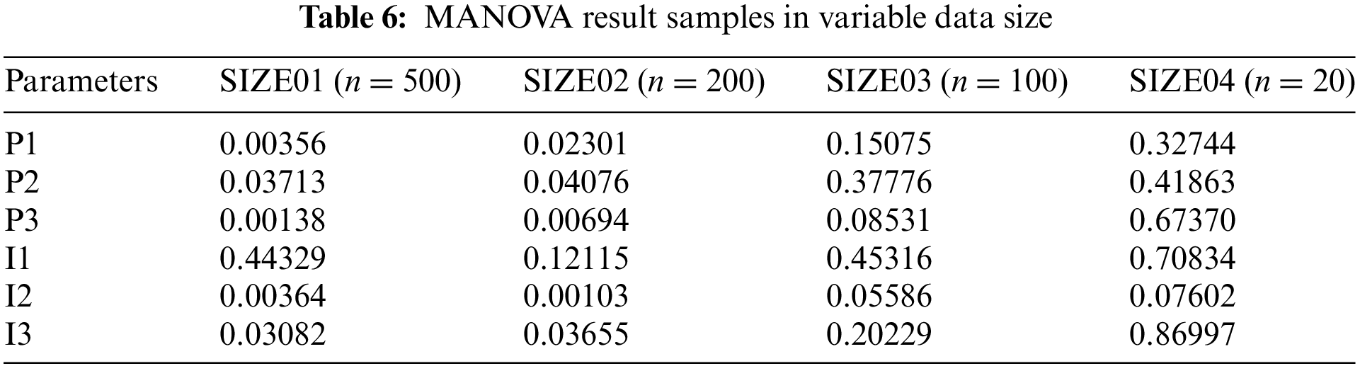
Where P1–P3 are the assembly parameters and I1–I3 are the interactions between parameters, as in shown in Table 7. n stands for the number of samples in different data sizes from a same scope of assembly parameter data, where data from SIZEm is contained in SIZEm−1. The variation of assembly parameters causes significant impact on the counterweight when P≤0.05. Otherwise the parameter is essentially irrelevant in traditional theory.

Where Interaction 1 is the interaction between flange edge height and bearing clearance, Interaction 2 is the interaction between flange edge height and curing coaxiality, and Interaction 3 is the interaction between dynamic balance and bearing clearance.

As illustrated in Table 6, the statistical significance pertaining to the counterweight and associated parameters exhibits considerable variation based on the size of the assembly data under analysis. Notably, the observed significance levels tend to decline as the quantity of available data for the parameters becomes limited: the relevance value P increases when the data size approaches at 200 and become implicit when the data size reached 100 and below. The proportion of relevant parameters in the total dispersion square sum may become inapparent under small size nonlinear data.

This deterioration of the analysis precision leads to the infeasibility of the association study on the assembly parameter data in practical application for the small batch assembly production of dynamic gyroscope. Given that the number of samples in each assembly batch is less than 20, conducting a MANOVA on in-line assembly data is infeasible. Therefore, it becomes imperative to predict the real-time assembly conditions to acquire information regarding the interactions of assembly parameters.

Furthermore, we conducted MANOVA on adequate historical assembly data to validate the interaction changing in assembly sequences and select relevant parameters for counterweight prediction. The dataset was partitioned into five subsets, each comprising 200 samples, in order to facilitate the subsequent analysis. The relevant significance between the parameter (with interactions included) and the counterweight is shown in Table 8.

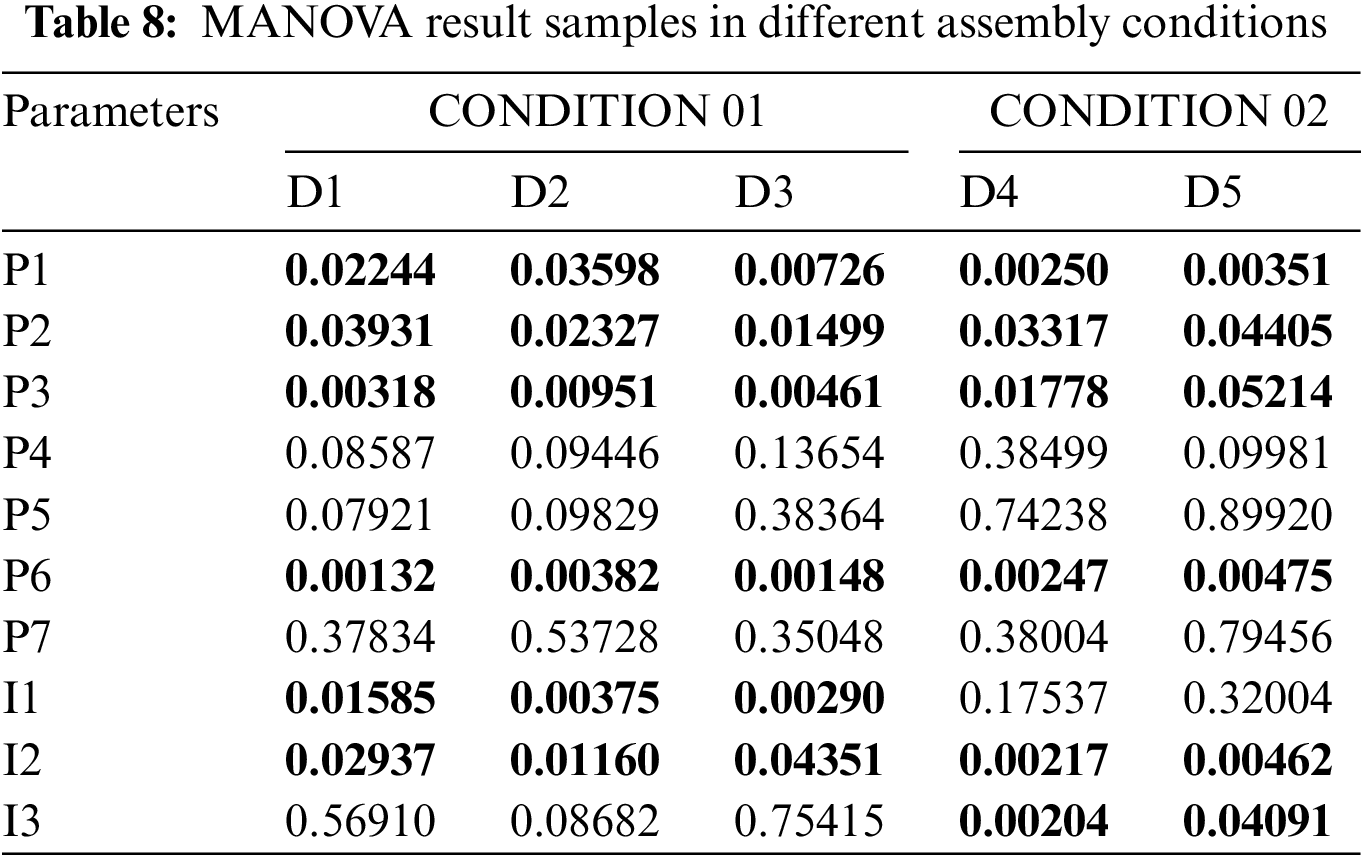
Where P1–P6 are the assembly parameters and I1–I3 are the interactions between certain parameters, as in shown in Table 7. D1–D5 are the subsets of gyroscope assembly sequences, covering parameter data from 200 gyroscopes in each batch.

As shown in Table 8, certain parameters shows significant relevance with the counterweight label in the assembly data subsets. Parameter P1, P2, P3 and P6 possess stable correlation with the label regardless the diversity of datasets. Meanwhile, the figure of interaction I1, I2 and I3 shows apparent variation in different assembly conditions: comparing to CONDITION 01, the relevant significance of I1 becomes implicit in CONDITION 02, in which interaction I3 shows a more remarkable association.

Unquantifiable deviation between the geometry and rotation center of gyroscope caused by manufacturing and assembling error, the interactions of assembly parameters are changing with the assembly sequences remarkably. We select the flange edge height, bearing clearance, curing coaxiality, preliminary dynamic balance and interactions in different assembly conditions as the input parameters for counterweight prediction.

In this study, the changing impact resulting from interactions is considered a form of parameter relation information and is input into the models to enhance learning ability under limited data for small-sample training. Therefore, for counterweight prediction in small-batch gyroscope assembly production, we initially introduce the assembly condition classification model. The training labels for this model are constructed through MANOVA analysis of historical assembly data, providing support for interaction data.

When historical data is scarce, the evaluation of the scalability of MANOVA for parameters should be conducted to confirm the minimal effective size for data analysis, such as the test in Table 8. We can still conduct effective MANOVA (or other data analysis methods) in few production batches, providing the minimum data we need.

4.3 Validation of the Dynamic Gyroscope Counterweight Prediction Method

In this paper, most common indicators are employed for the evaluation of the counterweight regression based on the ResGAT model. RMSE, mean absolute error (MAE), mean square error (MSE), mean absolute percentage error (MAPE), and coefficient of determination (R-Squared) are adopted to assess the prediction precision of the counterweight regression model [23].

In practical production processes, the internal standard for gyroscope dynamic balance debugging, in the specific gyroscope model under investigation, dictates that the error of the assembled counterweight should not exceed 10% of the actual counterweight value required by the gyroscope’s balance capability. Consequently, a predicted counterweight value within a ±10% residual of the actual required value is deemed a correct prediction. Therefore, the accuracy of the counterweight regression model can be expressed using formulas (31) and (32).

Accuracy=100%n∑i=1nCr(rd)(31)

Cr(rd)={1, if rd≤0.1⋅yi0,other(32)

where rd is the residual of the predicted counterweight value and yi is the required value.

In this study, we conducted a series of comparative experiments to validate the advantages of the proposed counterweight prediction method. The ResGAT model was trained for 500 epochs using the Adam optimizer. Subsequently, the model was tested with the dataset samples, and the counterweight regression results are presented in Fig. 9a.

Figure 9: Counterweight regression result of the ResGAT model

The predictive value is remarkably close to the true value of counterweight, which proves the effectiveness of the Multi-head ResGAT model.

To validate the superiority of the proposed counterweight prediction model comparing to traditional gyroscope counterweight empirical formulas, test results were contrasted with the empirical computed results based on corresponding primary dynamic balance figures, as seen in Fig. 9b and Table 9.

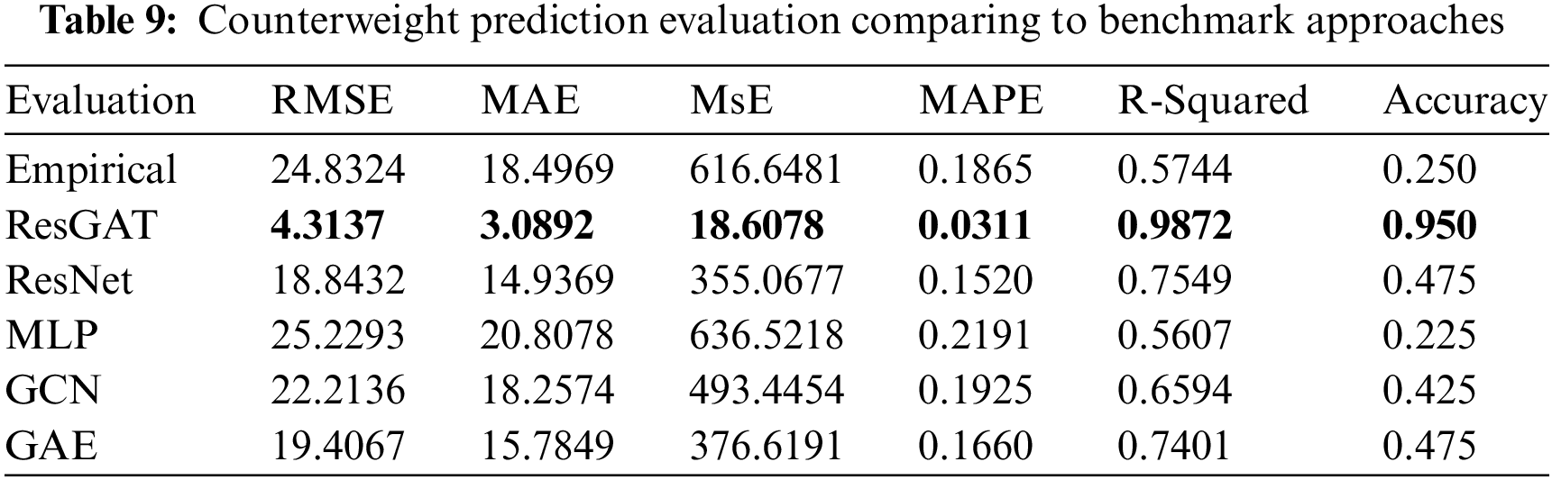
Compared to the traditional approach using empirical formulas, our proposed counterweight prediction model demonstrates significantly lower errors across all evaluation indicators. The consistently lower RMSE figure and higher accuracy affirm the superiority of our method, signaling efficiency improvements in gyroscope assembly.

To further validate the superiority of the GNN-based ResGAT method, comparative regression experiments are also conducted on the benchmark neural network models.

An ResNet model with similar residual network structure is utilized for comparison. Experiments are also conducted on traditional graph convolution network (GCN) and graph autoencoder (GAE) models, which are also GNN-based and capable of utilizing assembly graph data for interaction feature extraction. A traditional multi-layer perceptron (MLP) with similar neural weight amount is also utilized. The regression results and corresponding evaluation are shown in Fig. 10 and Table 9.

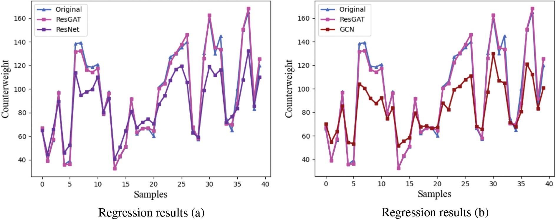
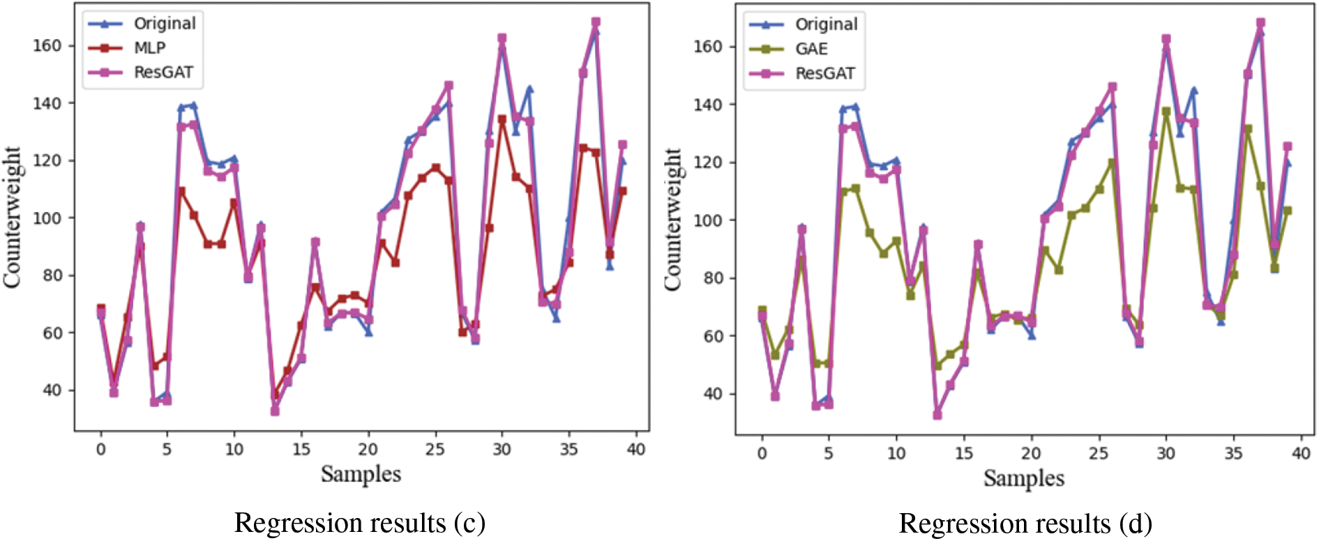
Figure 10: Competitive experiment results: (a) ResNet, (b) GCN, (c) MLP, (d) GAE

As shown in Fig. 10 and Table 9, in comparison with the model we propose, the traditional ResNet model has higher errors in RMSE, MAE, and MAPE, lower values in R-squared and significant lower accuracy, indicating its mediocre performance in counterweight prediction. The ResGAT model outperforms all other competing approaches, confirming the superiority of the gyroscope counterweight prediction method based on ResGAT.

GNN-based models is capable of utilizing interaction features as an isolated input when the correlation between input parameters changes with the data batches. These hidden changes is not easily learned for the traditional neural network, as it can be seen that the MLP is severely affected and achieves lower accuracy.

However, it is evident that both GCN and GAE also exhibit suboptimal performance in most indicators, even slightly worse than the ResNet model. When trained with small-sample assembly data, the graph convolution-based GCN and GAE lack robustness in addressing the overfitting problem, a challenge effectively mitigated by the attention mechanism and residual connection in ResGAT.

The ResGAT excels at extracting interaction features in the form of neural weights and demonstrates superior performance in avoiding overfitting under small-sample conditions, as compared to the graph attention mechanisms in GCN and GAT.

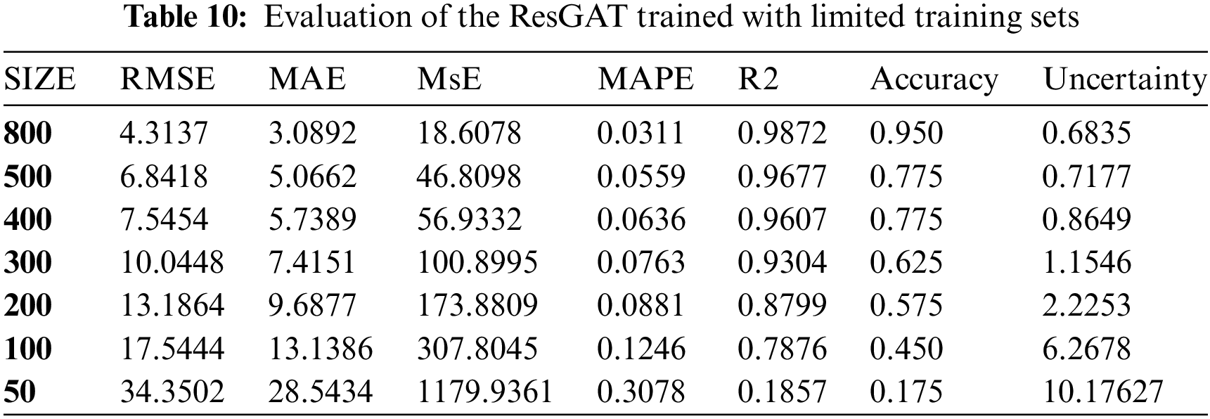
To further assess the model’s limitations under small sample conditions, we conduct additional controlled regression experiments, varying the size of the training set. For reliability evaluation, we utilize the type A evaluation of standard uncertainty to estimate regression reliability, as shown in formula (33) [24].

Uncertainty=∑j=1n(rj−r¯)2n−1(33)

where rj stands for the RMSE values in reduplicate experiments.

As shown in Table 10, the precision of counterweight regression reduces when the size of training set get smaller. According to the indicators, the accuracy of our model plunges when the training set size reaches 100 and shows under-fitting when it is limited to 50. Meanwhile, the uncertainty figures remain flat in the scope of 300–800 and suddenly rise when the size limited to 200 and below, which indicates that the model may become less reliable in these scenarios. Thus, in consideration of precession and reliability, our proposed ResGAT counterweight prediction model requires a minimum training set size larger than 200.

4.4 Validation of the SDAE-GPC Assembly Condition Classification Model

In view of the fact that the SDAE-GPC model incorporates assembly condition, it is imperative to select the input parameters of the model from the assembly processes prior to dynamic balance debugging. In previous assembly processes, parameters exhibiting significant variation characteristics in assembly sequences are selected for pattern recognition in order to identify the corresponding assembly conditions, as shown in Table 11.

In this paper, we focus on the classification of two main assembly conditions in the historical assembly data of the certain type of dynamic gyroscope. 1000 gyroscope assembly samples were divided on a scale of 4:1 to obtain the training and testing datasets. Table 12 describes the assembly condition classification task for the model.

Evaluating indicators are adopted to measure the classification accuracy of our SDAE-GPC model. In this paper, we employ accuracy, precision, recall, F1-score and AUC-score to evaluate the assembly condition classification [25,26].

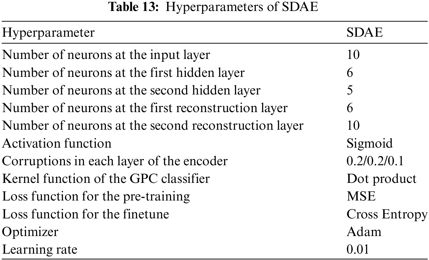
The hyperparameters of SDAE-GPC play significant roles in the performance of the classification model. We utilized an SDAE with three hidden layers, where the number of nodes was determined through experiments and parameter adjustments. The input layer consists of 10 neurons, corresponding to the dimensions of the normalized assembly parameters. The hyperparameters of SDAE-GPC are detailed in Table 13.

To confirm the SDAE-GPC classification model’s superiority, we conducted experiments with different classifiers, including SVM, gradient boosting decision tree (GBDT), and MLP. The MLP used in these experiments had a structure similar to the SDAE in the fine-tuning process, validating SDAE’s convergence priority. Initially, assembly condition classification experiments were performed solely on traditional classifiers. Subsequently, each of these classifiers was combined with SDAE for the same classification task.

SDAE models, with identical parameter settings, were pre-trained for 500 epochs to acquire denoising ability. Subsequent fine-tuning for 300 epochs was performed with different classifiers. The models were then tested on the test set and evaluated using the aforementioned indicators. The confusion matrices of the classification test results are shown in Fig. 11.

Figure 11: Confusion matrices of the classification results: (a) GBDT, (b) GPC, (c) SVM, (d) MLP (e) SDAE-GBDT, (f) SDAE-GPC, (g) SDAE-SVM, (h) SDAE-MLP

As shown in Fig. 11, the number of false samples in methods (a)–(d) is apparently higher than those in methods (e)–(h): more samples from CONDITION 01 are misclassified as CONDITION 02. When dealing with assembly condition classification, traditional classifier models are more easily affected by the noises in multiple input parameters and show poor robustness.

The evaluation of classification results are shown in Table 14.

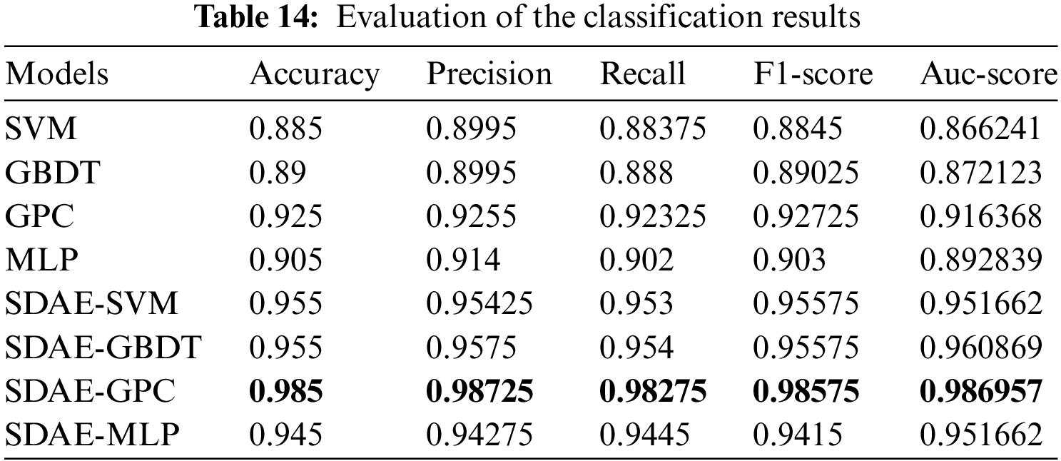
The evaluation results of the SDAE-GPC model in assembly classification significantly outperform all other methods across all indicators. SDAE-based classifiers demonstrate higher classification accuracy in various evaluation methods, confirming the denoising ability of SDAE. The GPC with a nonlinear kernel also exhibits advantages compared to SVM, GBDT, and MLP methods. This outcome underscores the superiority of the polynomial-kernel GPC in small-sample nonlinear assembly condition classification problems.

Furthermore, in comparison to MLP with conventional training, the SDAE-MLP trained using the pre-training and fine-tune strategy shows significant advantages in all indicators, affirming the superior convergence effect of its training procedure.

When historical data is unreliable for data analysis, such as situations when the significance of the parameter interactions changes with production batches, neural network models (such as the SDAE-GPC we propose) can be utilized for the prediction of the parameter correlation condition in small production batches.

Trained with sufficient parameter data and their corresponding correlation conditions (which are derived from data analysis in the minimal effective size), an efficacious neural network model is capable of predicting the parameter correlations without the in-time massive data required by traditional data analysis methods.

4.5 Validation of the Multi-Head ResGAT Counterweight Regression Model

In this paper, we utilized the data of a certain type of dynamic gyroscope with two certain corresponding assembly conditions. The correlated parameters and the interactions between them are expressed in form of graph data G=(A,X), which is shown in Tables 15 and 16.

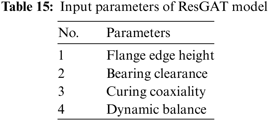
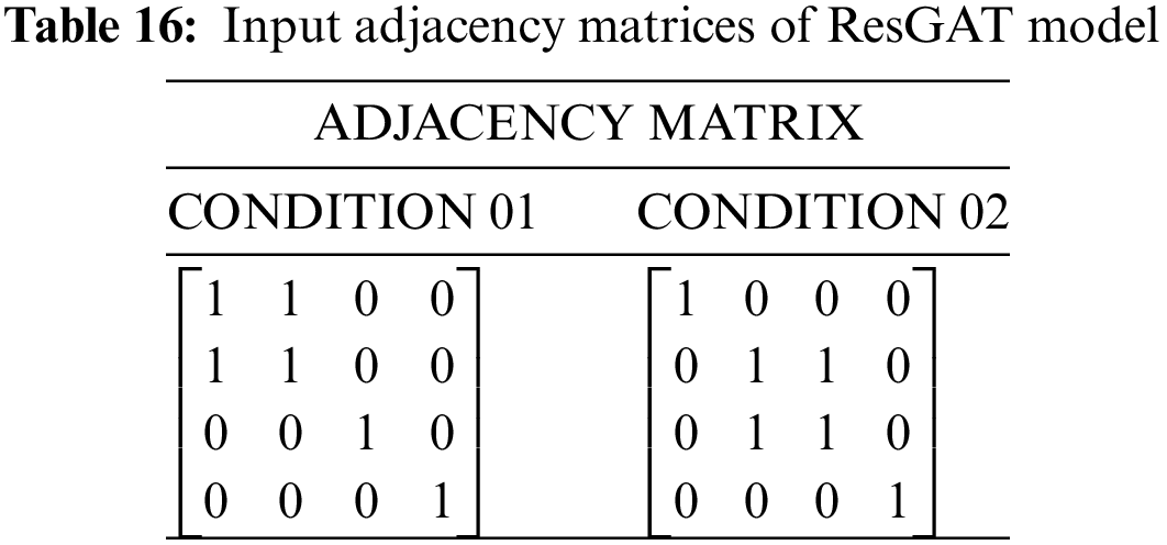
In Table 15, apart from the key parameter “primary dynamic balance” used in the empirical formulas, parameters No. 1 to No. 3 are all identified by MANOVA in Section 4.2. These parameters are derived from the gimbal assembly process, reflecting the potential deviation between the barycenter and rotation center. As shown in Table 16, the interactions among these parameters are illustrated in the adjacency matrices, which correspond to specific assembly conditions classified by the SDAE-GPC based on the preceding parameters of certain gyroscopes.

The precision of the proposed Multi-head ResGAT model is also highly affected by the hyperparameters we choose. After model structure adjustment based on commissioning tests, the hyperparameters of the regression model are listed in Table 17. The node numbers of the input layers in the feature extraction module and attention module are both 4, for the four parameter inputs of the assembly graph data.

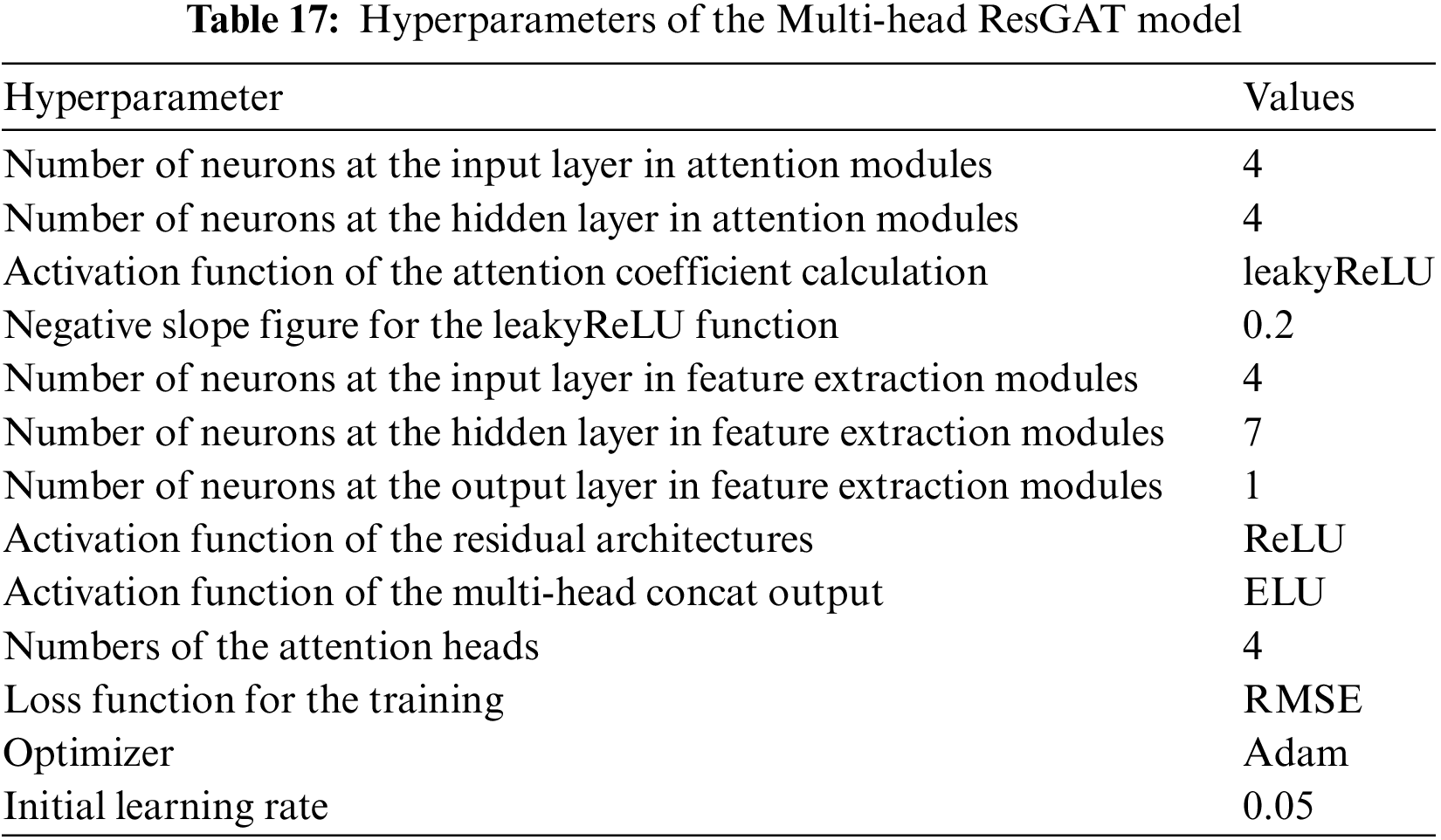
Key structural parameters are optimized via controlled experiments, in which nodes at the hidden layer in the feature extraction modules and numbers of attention heads are discussed. For each hyperparameter setting, 10 runs of repeated experiments were conducted to eliminate the randomness of algorithms, utilizing the test dataset of assembly parameters and corresponding counterweights. The results of the experiments are demonstrated in box-plots and shown in Figs. 12 and 13.

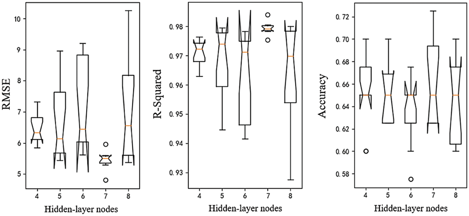
Figure 12: Boxplots of indicators for models over 10 runs in 5 different hidden nodes

Figure 13: Boxplots of indicators over 10 runs for models in 5 different attention heads

In Figs. 12 and 13, the model’s performance is significantly influenced by both hidden nodes and attention heads. The counterweight prediction achieves its highest precision when the number of hidden layer nodes is 7 and decreases when it reaches 8. Similarly, the model’s performance peaks when attention heads reach 4 but degrades notably when it reaches 5. Both of these performance declines are attributed to the increased complexity of the models, which can easily lead to overfitting under small-sample conditions. Therefore, the numbers of hidden layer nodes and attention heads are set to 7 and 4.

Additionally, to affirm the superiority of the SDAE-GPC-ResGAT counterweight prediction method, ablation experiments are conducted for a comprehensive comparison with benchmark models. Controlled experiments are carried out on different models, ranging from basic GAT to our composite SDAE-GPC-ResGAT model. Each innovation in the models is tested individually to elucidate the capabilities of our proposed model.

The original GAT model we employed has a structure and hyperparameters similar to the ResGAT. The two modifications from our model—optimized attention scores and residual connections for the GAT structure—are tested separately in the experiments.

The adjacency matrix inputs for these models are set to constant identity matrices. On the contrary, four additional sets of counterweight regression experiments are also conducted on ResGATs based on different assembly condition classifiers, which provide adjacency matrices for the ResGAT.

The prediction results of the comparative experiments are shown in Fig. 14, and the evaluation of the counterweight prediction results from competitive methods is presented in Table 18.

Figure 14: Regression results from GAT ablation experiments: (a) GAT-Modified 1, (b) GAT-Modified 2, (c) ResGAT, (d) C1-ResGAT, (e) C2-ResGAT, (f) C3-ResGAT, (g) C4-ResGAT

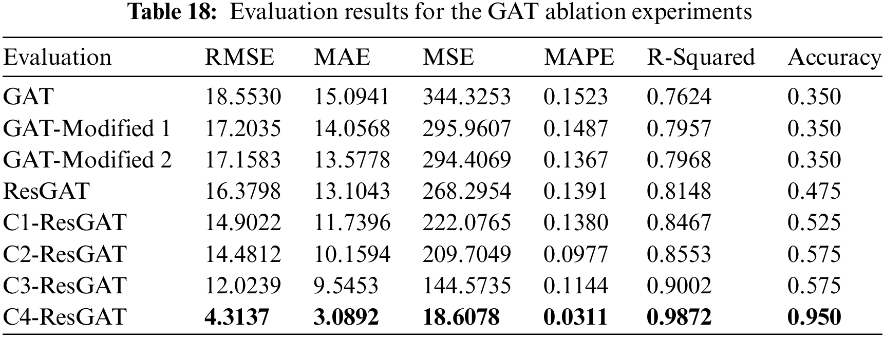
Where Modified 1 stands for the GAT model with optimized attention score and without residual connection, and Modified 2 stands for the GAT model with residual connection and original attention score calculation. C1 stands for SDAE-MLP, C2 stands for SDAE-GBDT, C3 stands for SDAE-SVM, and C4 stands for SDAE-GPC.

In Fig. 14 and Table 18, the regression results derived from the SDAE-GPC-ResGAT counterweight prediction method demonstrate the best performance in all evaluation indicators. This indicates that the model outperforms all other competing benchmark approaches, confirming the superiority of our proposed models.

The results of ablation experiments clearly show that GAT models with classification support have better precision, validating the effectiveness of assembly condition classification for counterweight prediction. However, the advantages of the ResGAT model are not significant enough due to the deficiency of interaction information. Further ablation experiments for the GAT models utilizing a similar SDAE-GPC classification model are conducted, as shown in Table 19.

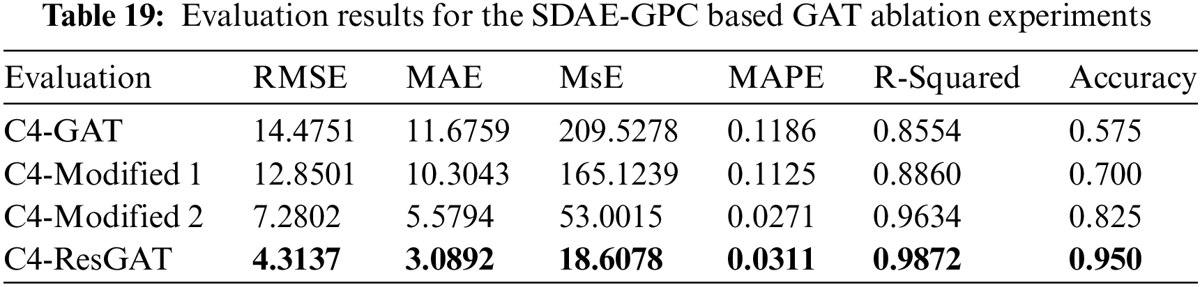
Comparing to the benchmark GAT model, all our modified models exhibit better counterweight regression precision. Among them, the ResGAT with both attention score and residual connection modifications shows the best performance. Modified 2 also achieves higher precision compared to traditional GAT models. The residual mappings capture differences between hidden layers of the graph neural network and learn residual information during the assembly parameter feature extraction process.

On the other hand, Modified 1 shows limited superiority but still outperforms the traditional GAT model. The modification in attention score proves effective in simplifying the graph attention mechanism, making the model applicable to the small-sample gyroscope assembly situation and preventing overfitting caused by a large number of neural weights.

As illustrated in Section 4.3, the internal standard for counterweight debugging is that the error of the counterweight should not exceed 10% of the required figure based on gyroscope dynamic balance. The over-proofed gyroscope will be disassembled for replacement of counterweight blocks, gimbal, and flange components. The assembly repetition rate of the experiments from different models is shown in Fig. 15.

Figure 15: Assembly repetition rate results for models

As depicted in Fig. 15, our experimental results on assembly repetition rate reveal an impressive assembly repetition rate of 5%. Notably, these prediction results surpass the performance of other existing methods and signifies a substantial enhancement in production efficiency. Such findings highlight the potential for enhancing production efficiency in the context of assembly line operations.

The proposed model is a versatile method suitable for various gyroscope models; however, there are a few limitations when applying the method to different assembly settings:

Correlation Analysis Requirement: Correlation analysis is essential to identify relevant assembly parameters for a new assembly setting. This implies the need for a dataset of minimal effective size for the association analysis procedure.

Re-Training Necessity: The model requires re-training with new assembly data whenever applied to a new assembly context. Although designed for small-sample industrial conditions, a certain amount of historical assembly data is still necessary for the training procedure.

5  Conclusion

In this research paper, we propose an innovative approach for predicting gyroscope counterweights during the dynamic gyroscope assembly process. Our methodology involves the development of an assembly condition classification model using a Stacked Denoising Autoencoder (SDAE) and Gaussian Process Classifier (GPC). This model generates crucial graph-based data, which serves as input for our gyroscope counterweight prediction method, employing a Multi-head Residual Graph Attention Network (ResGAT). Through comparative experiments using real-world assembly data from practical dynamic gyroscope production, our results underscore the effectiveness of the proposed method, highlighting its potential to enhance accuracy and efficiency in gyroscope counterweight prediction during assembly. Our approach offers a promising avenue for reducing labor hours and production costs in dynamic gyroscope assembly.

Looking ahead, our future work will address the few-shot problem, particularly in scenarios where historical assembly data is scarce. We aim to design models that leverage general features derived from assembly data of similar gyroscope models, utilizing transfer learning. Additionally, we plan to expand our dataset by collecting assembly data from various gyroscope models, enabling a comprehensive analysis of differences and similarities in their hidden feature space. If feasible, we intend to construct a general feature library for dynamic gyroscopes, optimizing our gyroscope counterweight prediction method for enhanced generalization and accuracy.

Acknowledgement: None.

Funding Statement: This research was supported by the National Natural Science Foundation of China (No. 51705100) and the Foundation of Research on Intelligent Design Method Based on Knowledge Space Reconstruction and Perceptual Push (No. 52075120).

Author Contributions: The authors confirm contribution to the paper as follows: Wuyang Fan designed and conducted the experiments and wrote the paper manuscript. And Prof. Shisheng Zhong read the article.

Availability of Data and Materials: The authors are not authorized by related enterprise to supply corresponding data.

Conflicts of Interest: The authors declared that they have no known competing financial interests or personal relationships that could have appeared to influence the work reported in this paper. We declare that we do not have any commercial or associative interest that represents a conflict of interest in connection with the work submitted.

References

1. Li, Y. X., Xi, B. Q., Ren, S. Q., Wang, C. H. (2023). Precision enhancement by compensation of hemispherical resonator gyroscope dynamic output errors. IEEE Transactions on Instrumentation and Measurement, 72, 1–10. [Google Scholar]

2. Rudy, R. Q., Hauser, C., Knight, R. R., Pulskamp, J. S. (2023). Dynamic quality factor equalization for improved bias stability in mode-matched gyroscopes. 2023 IEEE International Symposium on Inertial Sensors and Systems (INERTIAL), vol. 72, pp. 1–4. Lihue, HI, USA, IEEE. [Google Scholar]

3. Zhou, S., Chen, J. (2005). Research on dynamic balance method for gyro rotor of seeker, pp. 1673–5048. Aero Weaponry, AVIC, Henan, China. [Google Scholar]

4. Tu, Y. H., Peng, C. C. (2020). An ARMA-based digital twin for MEMS gyroscope drift dynamics modeling and real-time compensation. IEEE Sensors Journal, 21(3), 2712–2724. [Google Scholar]

5. Dodge, Y. (2006). Coefficient of determination. Alphascript Publishing, 31(1), 63–64. [Google Scholar]

6. Grimm, L. G., Nesselroade Jr, K. P. (2019). Statistical applications for the behavioral and social sciences (No. 175344). New Jersey, John Wiley & Sons. [Google Scholar]

7. Chakraborty, N., Sakhanenko, L. (2023). Novel multiplier bootstrap tests for high-dimensional data with applications to MANOVA. Computational Statistics & Data Analysis, 178, 107619. [Google Scholar]

8. Danixeb, Lakens, L. (2013). Calculating and reporting effect sizes to facilitate cumulative science: A practical primer for t-tests and ANOVAs. Frontiers in Psychology, 4, 863. [Google Scholar]

9. Cox, C. (2010). The generalized f distribution: An umbrella for parametric survival analysis. Statistics in Medicine, 27(21), 4301–4312. [Google Scholar]

10. Abiodun, O. I., Jantan, A., Omolara, A. E., Dada, K. V., Mohamed, N. A. et al. (2018). State-of-the-art in artificial neural network applications: A survey. Heliyon, 4(11), e00938. [Google Scholar] [PubMed]

11. Fang, Y., Fu, W., An, C., Yuan, Z., Fei, J. (2021). Modelling, simulation and dynamic sliding mode control of a mems gyroscope. Micromachines, 12(2), 190. [Google Scholar] [PubMed]

12. Luo, S., Yang, G., Li, J., Ouakad, H. M. (2022). Dynamic analysis, circuit realization and accelerated adaptive backstepping control of the FO MEMS gyroscope. Chaos, Solitons & Fractals, 155, 111735. [Google Scholar]

13. Xu, Y. K., Tan, J. R., Mei, T., Zhou, J. S., Tang, H. L. et al. (2019). The performance prediction of coordinator based on prior knowledge of multibody dynamics and kernel method. Flight Control & Detection, (4), 55–61 (In Chinese). [Google Scholar]

14. Zhang, R., Xu, B., Wei, Q., Yang, T., Zhao, W. et al. (2020). Serial-parallel estimation model-based sliding mode control of MEMS gyroscopes. IEEE Transactions on Systems, Man, and Cybernetics: Systems, 51(12), 7764–7775. [Google Scholar]

15. Cao, H., Cui, R., Liu, W., Ma, T., Zhang, Z. et al. (2021). Dual mass MEMS gyroscope temperature drift compensation based on TFPF-MEA-BP algorithm. Sensor Review, 41(2), 162–175. [Google Scholar]

16. Vaswani, A., Shazeer, N., Parmar, N., Uszkoreit, J., Jones, L. et al. (2017). Attention is all you need. in Proceedings of the 31st International Conference on Neural Information Processing Systems, pp. 6000–6010. [Google Scholar]

17. Kipf, T. N., Welling, M. (2016). Semi-supervised classification with graph convolutional networks. arXiv preprint arXiv:1609.02907. [Google Scholar]

18. Hong, Q. J., Ushakov, S. V., van de Walle, A., Navrotsky, A. (2022). Melting temperature prediction using a graph neural network model: From ancient minerals to new materials. Proceedings of the National Academy of Sciences, 119(36), e2209630119. [Google Scholar]

19. Velickovic, P., Cucurull, G., Casanova, A., Romero, A., Lio, P. et al. (2017). Graph attention networks. Stat, 1050(20), 10–48550. [Google Scholar]

20. Kipf, T. N., Welling, M. (2016). Variational graph auto-encoders. arXiv preprint arXiv:1611.07308. [Google Scholar]

21. Vincent, P., Larochelle, H., Lajoie, I., Bengio, Y., Manzagol, P. A. (2010). Stacked denoising autoencoders: Learning useful representations in a deep network with a local denoising criterion. Journal of Machine Learning Research, 11(12), 3371–3408. [Google Scholar]

22. Liu, D., Zhong, S., Lin, L., Zhao, M., Fu, X. et al. (2022). Highly imbalanced fault diagnosis of gas turbines via clustering-based downsampling and deep siamese self-attention network. Advanced Engineering Informatics, 54, 101725. [Google Scholar]

23. Kariampuzha, W. Z., Alyea, G., Qu, S., Sanjak, J., Mathé, E. et al. (2023). Precision information extraction for rare disease epidemiology at scale. Journal of Translational Medicine, 21(1), 157. [Google Scholar] [PubMed]

24. Bich, W., Cox, M., Michotte, C. (2016). Towards a new GUM—An update. Metrologia, 53(5), S149. [Google Scholar]

25. Nguyen, N. D., Tan, W., Du, L., Buntine, W., Beare, R. et al. (2023). AUC maximization for low-resource named entity recognition. Proceedings of the AAAI Conference on Artificial Intelligence, vol. 37, no. 11, pp. 13389–13399. [Google Scholar]

26. Chicco, D., Warrens, M. J., Jurman, G. (2021). The coefficient of determination R-squared is more informative than SMAPE, MAE, MAPE, MSE and RMSE in regression analysis evaluation. PeerJ Computer Science, 7, e623. [Google Scholar] [PubMed]