MPI/OpenMP-Based Parallel Solver for Imprint Forming Simulation

1  Introduction

The field of imprint forming has adopted the numerical simulation method due to the rapid development of computer technology. For instance, Xu et al. developed a special-purpose simulation system named CoinForm for the embossing process of commemorative coins and compared it with the results of Deform-3D software to verify its excellent performance [1]. Zhong et al. extended the work of Xu et al. to study the mechanism of the flash line of silver commemorative coins by proposing a novel radial friction work (RFW) model to predict the tendency of flash lines [2]. Li et al. proposed a multi-point integration-based lock-free hexahedral element for coining simulation in which a new adaptive subdivision method was applied [3]. The obtained results agreed well with the experiments. Alexandrino proposed a novel finite element (FE) method to predict and optimize the die stress at the end of the stroke, aiming to extend the service life of the coining dies [4]. He and his co-workers verified the feasibility of the finite element method to predict material flow and filling of the intricate reliefs of coins, and to predict the required coin minting forces before fabricating the actual dies [5]. Afonso et al. established a bi-material model with a polymer center and a metal ring by using the FE method, which proved the effectiveness of the mechanical joint resulting from the interface contact pressure between the polymer and the metal [6]. Peng et al. simulated and analyzed the stress distribution and material flow in the coining process of single or bi-material with the assistance of Deform-3D, and analyzed the reason for falling off the inner core of the coin [7]. Almost all finite element programs used in the above research are based on serial computation, except for Zhong et al. [2] and Li et al. [3] where open multi-processing (OpenMP) is adopted. Even in the framework of the OpenMP codes, the data race of calculating internal forces significantly reduces the efficiency of the parallel solver. Although the professional metal forming software Deform-3D could provide parallel computing, it limits the number of elements when meshing solid objects, and thus can not satisfy the increasing requirements for coins with complex tiny features that millions of solid elements are present. In the present work, parallel programs named CoinFEM for complicated coins are developed for simulating at least 7 million tetrahedron elements involved in coining modeling.

At present, there are two main parallel programming models, namely distributed memory processing (DMP) and shared memory processing (SMP) [8]. In the case of DMP, each processor has its memory and uses message-passing interfaces for communication. The utilization of multiple address spaces, as in message passing interface (MPI), can enhance portability but can also lead to increased programming complexity, as stated by [9–11]. On the other hand, in SMP systems, where several processors share a single address space, programming becomes simpler but portability may be reduced, as mentioned by [12–15] in the case of OpenMP and Pthreads. The development of parallel solvers for simulating minting in a single computer has gained significant attention due to the rapid progress of multi-core technology. As the mint industry is highly confidential, the protection of newly designed product data is paramount, and implementing simulation procedures in a remote large-scale cluster poses risks. Therefore, this study investigates parallel technology for carrying out computations in multi-core computers and local small-scale clusters. Adopting parallel computing in the coining process offers three key advantages. Firstly, the solver that utilizes the dynamic explicit central difference algorithm involves a vast number of node and element loops, rendering it suitable for OpenMP. Secondly, the symmetrical physical structure of commemorative coins allows for partitioning different regions, making it a viable option for MPI. Finally, multiple computing cores becoming common for individual and industrial users.

Most high-performance computing (HPC) architectures include multi-core CPU clusters interconnected through high-speed networks that support hierarchical memory models, and support shared memory within a single compute node and distributed memory across different compute nodes [16–18]. The hybrid MPI/OpenMP parallel programming model combines distributed memory parallelization on node interconnection and shared memory parallelization within each compute node. Undoubtedly, at higher parallel core counts, hybrid parallelism has advantages over pure MPI parallelism or pure OpenMP parallelism. However, the development of numerical analysis for commemorative coin simulations has been slow due to confidentiality concerns. Therefore, based on the original commemorative coin dynamic explicit central difference algorithm solver, this paper proposes three parallel computing solvers to study the efficiency and accuracy of the mint company, namely pure MPI, pure OpenMP, and hybrid MPI/OpenMP.

The remaining article is structured in the following manner. Section 2 primarily focuses on introducing the dynamic explicit central difference finite element method algorithm utilized for simulating commemorative coins. In Section 3, we discuss the implementation methods of pure MPI, pure OpenMP, and hybrid MPI/OpenMP modes parallelization for the coining process, with particular emphasis placed on enhancing parallel efficiency. Section 4 validates the correctness of the parallel solvers by comparing their results with experimental data and those from serial computations and also analyzes the speedup ratios of the three parallel schemes. Finally, Section 5 presents a summary of the findings.

2  Dynamic Explicit Central Difference Algorithm

The process of imprint forming can be considered a quasi-static procedure [1,19,20]. Consequently, we can describe it by using the following governing equation:

σ⋅∇+ρb=ρu¨+cu˙(1)

where the boundary conditions are as follows:

(n⋅σ)∣Γt=t¯,u∣Γu=u¯(2)

Here, σ represents the Cauchy stress, b denotes the body force, ρ indicates the current material density, u is the displacement, u˙ stands for the velocity, u¨ represents the acceleration, c is for the damping coefficient, Γt and Γu denote the traction boundary and displacement boundary, respectively. Moreover, t¯ signifies the traction acting on Γt, and u¯ represents the displacement constraint on Γu. Additionally, n refers to the elemental outward normal of boundary Γt.

By introducing virtual displacement δu, the weak form of the motion equation, Eq. (1), could be obtained by the weighted residual method, integration by part and divergence theorem,

∫Ωρu¨iδuidΩ+∫Ωcu˙iδuidΩ+∫Ωσijδui,jdΩ−∫ΩρbiδuidΩ−∫Γtt¯iδuidΓ=0(3)

where i and j indicate the components of the spatial variables following the Einstein summation convention.

In this research, the dynamic explicit central difference algorithm for imprint forming is based on the second-order tetrahedral elements, where each element has ten tetrahedral nodes. The expressions of its shape functions are given as

r1=1−r−s−t,r2=r,r3=s,r4=t(4)

where r, s and t are the local coordinates of any point in one elemental region. Thus, the expressions for the interpolation shape functions are given as

N1=r1(2r1−1),N2=r2(2r2−1),N3=r3(2r3−1),N4=r4(2r4−1),N5=4r1r2,N6=4r2r3,N7=4r3r1,N8=4r1r4,N9=4r2r4,N10=4r3r4(5)

The matrix format of the elemental shape function is written as

N=[IN1,IN2,IN3,IN4,⋯,IN10](6)

where I is an identity matrix of 3×3.

The strain gradient matrix is expressed as

B=LN(7)

where the strain gradient operator is written as

LT=[∂∂x00∂∂y0∂∂z0∂∂y0∂∂x∂∂z000∂∂z0∂∂y∂∂x](8)

The strain vector is expressed as

ε=(εx,εy,εz,εxy,εyz,εzx)T=Bu(9)

The coordinate x, displacement u, velocity u˙ and acceleration u¨ of any point in the element can be obtained by interpolation of shape function N

{x=[x1,x2,x3]T=Nxeu=[u1,u2,u3]T=Nueu˙=[u˙1,u˙2,u˙3]T=Nu˙eu¨=[u¨1,u¨2,u¨3]T=Nu¨e(10)

where xe, ue, u˙e, u¨e are the coordinate, displacement, velocity and acceleration of each node of an element e. For example, the coordinate vector xe can be written as

xe=(x1T,x2T,⋯,x10T)T,xi=(xi,yi,zi)T(11)

There are similar expressions for interpolating the other physical quantities of the point (r,s,t).

By inserting Eqs. (6)–(10) into the formula for the virtual work principle (Eq. (3)), the resulting equation is

∫ΩρNTNdΩU¨+∫ΩcNTNdΩU˙=∫ΩNTbdΩ−∫ΩBTσdΩ(12)

where

M=∫ΩρNTNdΩ,C=∫ΩcNTNdΩ,P=∫ΩNTbdΩ,F=∫ΩBTσdΩ(13)

Finally, we rewrite Eq. (12) as

MU¨+CU˙=P−F(14)

where P and F are the external and internal forces, respectively. U¨ and U˙ are the global matrices nodal velocity and acceleration. In the dynamic explicit integration algorithm, a lumped mass matrix is employed, where M is a diagonal matrix, and the damping matrix C is taken as αM, with α typically set to 0.1.

Consequently, the momentum equation (Eq. (14)) is decoupled using the lumped mass matrix and can be explicitly solved by solving the following equation:

miu¨+αmiu˙=Pi−Fi(15)

where mi represents the nodal mass.

Eq. (15) is usually solved by the central difference algorithm. Suppose that the state at time t is n, the physical quantities at time t and before time t are known. Define t−Δt, t−Δt/2, t+Δt and t+Δt/2 as states n−1, n−1/2, n+1 and n+1/2, respectively. Assume that the increments of the two-time steps before and after time t are different, that is, Δt≠Δtn−1. Let β=Δtn/Δtn−1. The velocity and acceleration obtained by the central difference method are as follows:

u˙n=β1+βu˙n+1/2+11+βu˙n−1/2(16)

u¨n=2(1+β)Δtn−1(u˙n+1/2−u˙n−1/2)(17)

The displacement at time t+Δt can be updated by the following equation:

un+1=un+u˙n+1/2⋅Δtn(18)

Substituting Eqs. (16) and (17) into Eq. (15), we can get

u˙n+1/2=BiAiu˙n−1/2+1AiGn(19)

where

Ai=2mi+αβmiΔtn−1(1+β)Δtn−1,Bi=2mi−αmiΔtn−1(1+β)Δtn−1,Gn=Pn−Fn(20)

Finally, we rewrite Eq. (19) as

u˙n+1/2=2−αΔtn−12+αβΔtn−1u˙n−1/2+(1+β)Δtn−1(2+αβΔtn−1)mi(Pn−Fn)(21)

Eqs. (18) and (21) offer explicit calculation formats for nodal displacement and velocity when the displacement and velocity from the previous two steps are known. In the initial step, direct utilization of Eqs. (18) and (21) is not feasible due to the unknown velocity u˙n−1/2 at the time t−Δt/2. However, the initial conditions for displacement and velocity before the start of the coining process are typically known, namely

u0=0,u˙0=0(22)

Letting Δt0=Δt0−1, that is, β=1. From the above initial velocity conditions Eqs. (22) and (16), the velocity vector at 0−1/2 time can be obtained as

u˙0−1/2=−u˙0+1/2(23)

Substituting Eq. (23) into Eq. (19), we can get the calculation expression for nodal velocity in the first incremental step as

u˙0+1/2=Δt02mi(P0−F0)(24)

After applying the central difference algorithm, the explicit Eq. (15) is solved to obtain the velocities of each node. The geometrical shape of the workpiece is then updated based on this solution. At each time step, various factors such as internal force, friction force, contact force, velocity, and displacement of each node, as well as stress and strain of each element and material response history, are updated through nodal and elemental loop calculations. These calculations are numerous, making the algorithm ideal for parallel OpenMP computing. Additionally, the initial workpiece’s symmetric geometry allows for MPI partitioning.

To ensure the stability of calculations, it is crucial to limit the size of the time increment step Δt because of the conditional stability of the central difference algorithm. The time increment step size that meets the stability condition can be estimated by approximating the minimum travel time of the expansion wave over any element.

Δt⩽γLnec(25)

where γ denotes the reduction factor, taking value of 0.5∼0.8; c is the propagation speed of expansion wave in the material, defined as c=E/ρ, with E being the elastic modulus and ρ as the current material density; Lne is the nominal length of the element e at the time step tn. Specifically for tetrahedral elements, the minimum nominal length of the element can be characterized as the minimum distance from the four nodes of the element to its corresponding face.

3  Parallel Programming for Coining

3.1 MPI Parallel Programming Technology

MPI is a library for message passing, which facilitates communication and coordination between multiple processes in a distributed memory system. This enables parallel computing and offers a range of functions and syntax for programming parallel programs [21–23]. In this work, the parallel solver utilizes MPICH (a freely available, portable implementation of MPI) to configure the MPI environment, and uses blocking communication mode for data transmission. The basic idea of the MPI parallel algorithm for the coining process is as follows.

Initially, all processes commence by invoking the MPI initialization function, and each process acquires a unique identifier for distinguishing among other processes. Then, the elements of the target workpiece are divided into np equal parts according to certain rules of load balance (where np is the number of cores specified by the user). Due to its symmetrical geometry, the initial workpiece can be easily divided into any divisions with an almost equal number of elements. The partitioned graphic is shown in Fig. 1.

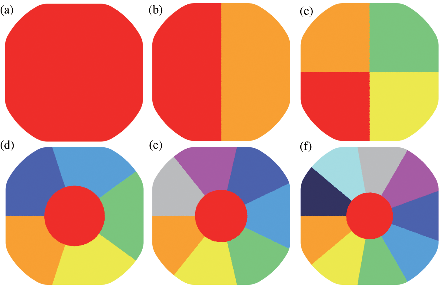
Figure 1: Partition diagram of the workpiece. Panel (a) represents the workpiece without parallel; Panels (b), (c), (d), (e) and (f) represent the partitions of the workpiece in cases of np=2, np=4, np=6, np=8 and np=10, respectively

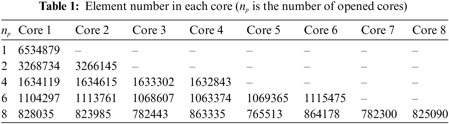
Secondly, the physical information of each workpiece’s elements (including element connectivity and node coordinates) within each subdomain is transmitted to its corresponding core. This establishes a one-to-one mapping between cores and subdomains and allows for the construction of boundary connections between different cores. For instance, if we consider a model with 6.5 million elements, Table 1 lists the element numbers found in the relevant cores.

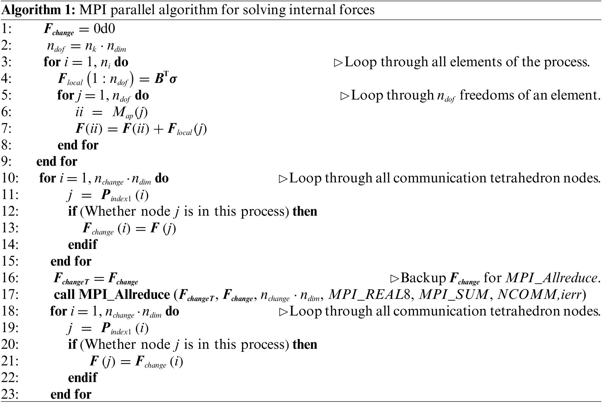
Finally, each subdomain completes a series of calculations, including the computation of nodal internal and frictional forces, contact determination for each workpiece node, updates to node information (e.g., coordinates and speed), updates to stress and strain in each subdomain’s elements, determination of time step, and output of results. The specific steps involved in the MPI parallel calculation for the imprint-forming solver are presented in Fig. 2. The functions performed by each used core, which include reading input data, initializing, calculating, and outputting, are the same, as shown in Fig. 2. Additionally, during the partitioning process, adjacent elements are separated into different cores but share the same tetrahedron nodes (The junction of different colors as shown in Fig. 1). However, the physical quantity of these nodes should be accumulated by different elements sharing the same tetrahedron nodes during the calculation. To ensure the physical quantity’s correctness, MPI parallel data communicating command MPI_Allreduce needs to be added to facilitate communication between different cores.

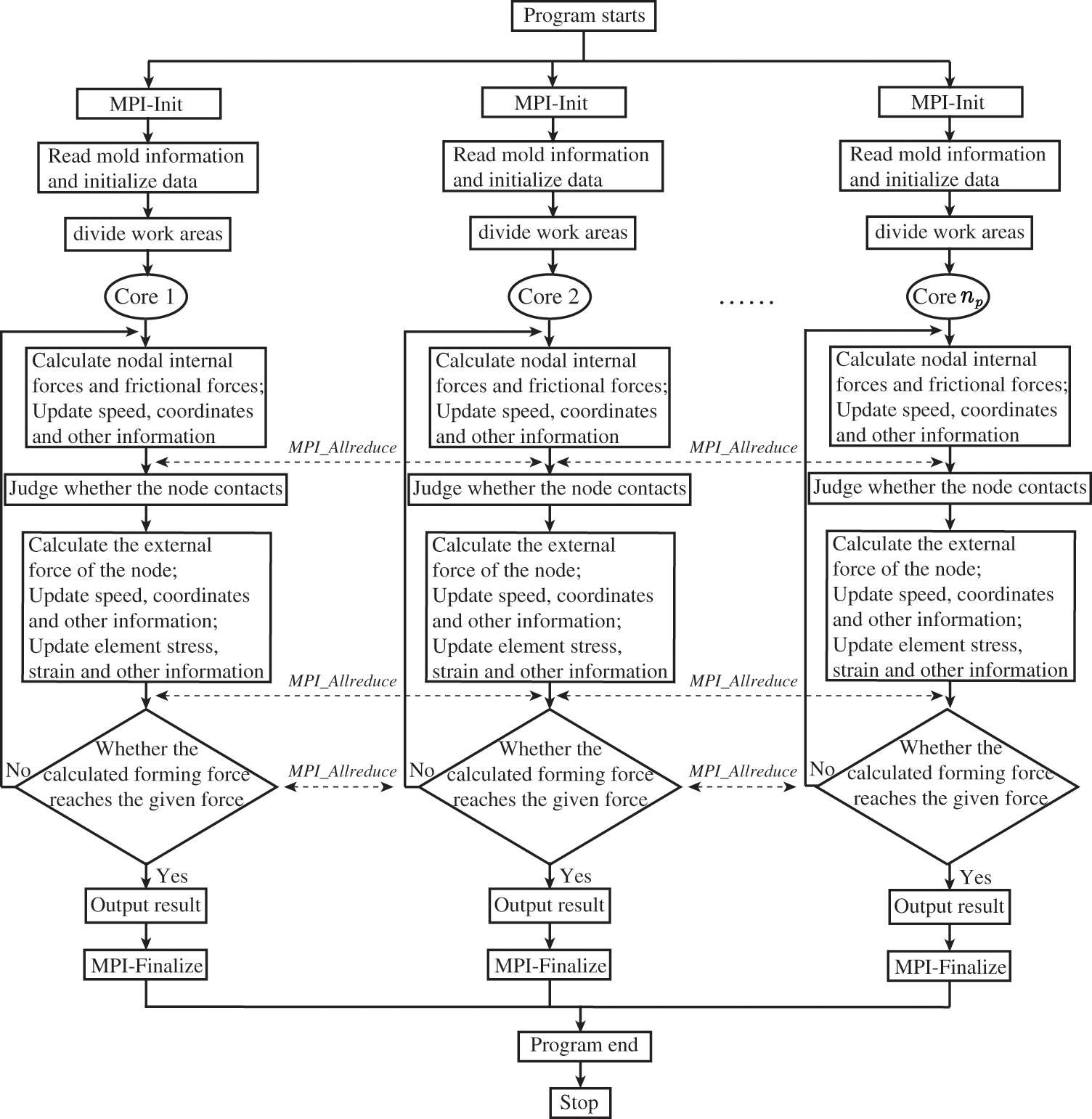
Figure 2: Flow chart of MPI parallel computing for coining simulation. MPI_Allreduce is used for message passing between different cores

Assume that the number of MPI processes is np, and the numbers of elements and nodes of the workpiece after the partition are ni and pi, respectively (the numbers of ni and pi of each process are different). In this research, the number of nodes per tetrahedron element takes the value of nk=10 and the dimension of the physical problem takes the value ndim=3, then the degree of freedom of each element takes the value of ndof=nk⋅ndim. The array Map(ndof) maps the local degrees of freedom in an element into the corresponding global degrees of freedom. Identify all nodes necessitating communication, totaling nchange, and store these nodes in Pindex1 which holds the global node numbering of the communication tetrahedron nodes. The sizes of F, Fchange and FchangeT are pi⋅ndim, nchange⋅ndim and nchange⋅ndim, respectively. Flocal is an array with the size of ndof that temporarily stores the internal forces of a single element. The pseudo-code of the MPI parallel process for calculating the internal forces of elemental nodes is illustrated in Algorithm 1.

Excessive communication can negatively impact parallel efficiency; therefore, optimizing communication between cores is necessary once result accuracy is guaranteed [24]. In this study, the communication balance is maintained because each core boundary has a similar number of elements, as shown in Fig. 1.

3.2 OpenMP Parallel Programming Technology

The OpenMP parallel is a programming interface designed for parallel programming in shared memory systems, which operates using a fork-join model. Upon encountering an OpenMP directive, the system generates or awakes a new set of threads to execute tasks in parallel regions. Once all the threads have completed executing the parallel tasks, the parallel computation terminates, and the main thread resumes continuous operation while the other threads either sleep or shut down [25–28]. The Visual Studio 2019 integrated with Intel Fortran 2021 OpenMP environment is used to implement this parallel solver. Here are some specific concepts of OpenMP parallel programming that can be utilized for coin simulation.

Firstly, the OpenMP parallel environment is initialized, which enables the primary thread to obtain information about the mold and workpiece and initialize the relevant calculation data. Unlike the MPI parallel algorithm, there is no requirement to partition the workpiece target. Subsequently, any statement containing loops over tetrahedron nodes or elements can be parallelized by using an OpenMP directive. This includes calculations for internal forces and friction forces of the nodes, as well as updates to nodal velocity and coordinates, and elemental stress, strain, equivalent stress, and equivalent strain. Assume that the number of open threads is nnump, and the element and nodal numbers of the workpieces are n and p, respectively. The pseudo-code of the OpenMP parallel process for calculating the internal forces of nodes is shown in Algorithm 2.

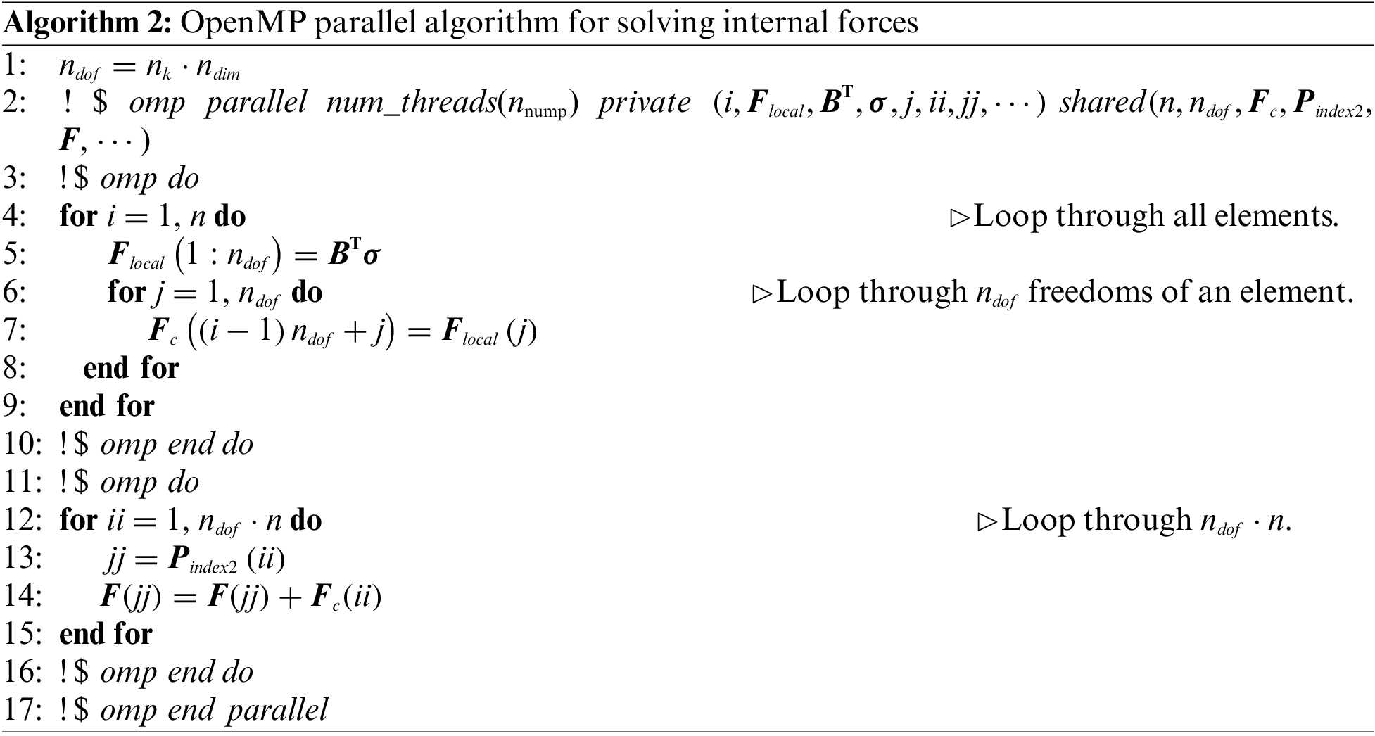
In this algorithm, the array F is utilized to store the global nodal internal forces, while Fc is an intermediate array used to hold the internal forces of the local tetrahedron nodes. The definitions of nk, ndim, ndof and Flocal are same as those in Algorithm 1. The sizes of F and Fc are p⋅ndim and ndof⋅n, respectively. Pindex2 is used to map internal forces from Fc to F.

During the internal force-solving loop, the initial calculation of the element loop only acquires the local node’s internal force, which must be mapped to the corresponding global tetrahedron node. However, introducing parallelism may cause data race problems because different threads read and write to the same location in a shared array. Such data races can substantially affect parallel efficiency [25,29].

To mitigate this type of data race, we have introduced a large intermediate array Fc in parallel computing, which holds the internal forces of local nodes. Once all the internal forces of local nodes are calculated and passed into Fc, forces in the intermediate array are mapped back to F. This mapping can be either parallel or serial, depending on the amount of calculation required, but the impact on code efficiency can be ignored.

Finally, the computation moves forward, and the outcome is produced by the main thread. Fig. 3 illustrates the OpenMP parallel computing process used for solving other physical quantities in the imprint-forming solver.

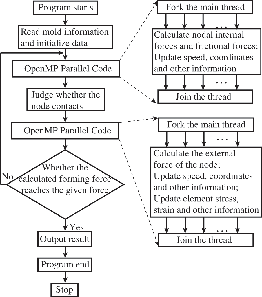
Figure 3: Chart of OpenMP parallel computing process

3.3 Hybrid MPI/OpenMP Parallel Programming Technology

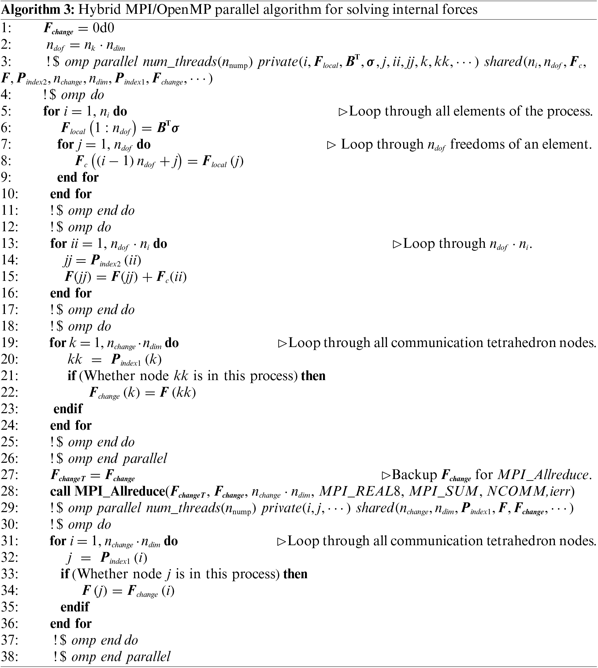
MPI is highly effective for handling coarse-grained parallelism with minimal overhead, while OpenMP excels in managing fine-grained parallelism. The MPI parallel computing model, focusing on pure implementation, provides scalability across multiple compute nodes and eliminates data placement concerns. Nevertheless, it poses challenges in terms of development, debugging, explicit communication, and load balancing. On the other hand, the pure OpenMP parallel computing model enables easy parallelism, low latency, and high bandwidth but is limited to shared memory machines and single compute nodes [30–33]. Thus, it is evident that both MPI and OpenMP have their respective limitations. To achieve enhanced acceleration effects, this research introduces a hybrid MPI/OpenMP parallel computing scheme for the dynamic explicit central difference algorithm. The hybrid MPI/OpenMP parallel solver leverages multiple compute nodes, allowing communication between MPI processes within the same node or across different compute nodes. The concrete implementation of the hybrid MPI/OpenMP parallel solver in this article involves employing OpenMP parallelism for loop statements while building upon the initial MPI parallel solver. This entails creating or activating OpenMP threads within the loop section of each MPI process. It is important to note that the communication between MPI processes does not utilize OpenMP parallelism. For further insights into the implementation, refer to Sections 3.1 and 3.2, as depicted in Fig. 4.

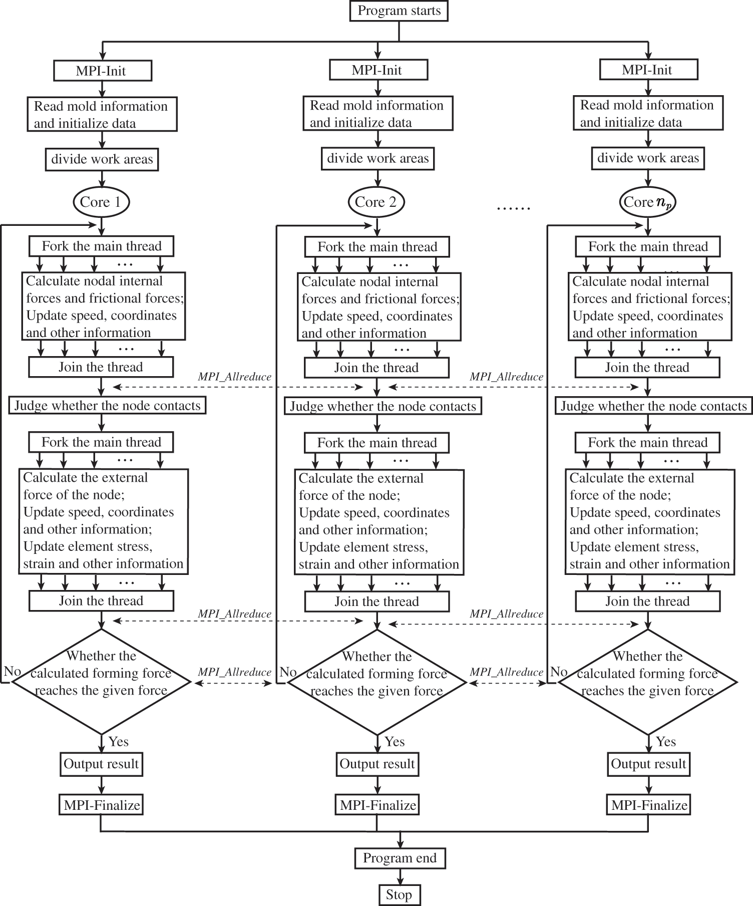
Figure 4: Chart of hybrid MPI/OpenMP parallel computing process

Assuming the number of MPI processes and OpenMP threads are denoted by np and nnump, respectively, the algorithm employs the same definitions as those in Algorithm 1 for variables such as ni, pi, nk, ndim, ndof, nchange, F, Flocal, Fchange, FchangeT, and Pindex1. Additionally, the definitions of Fc, Pindex2, and Flocal remain consistent with those in Algorithm 2. The pseudo-code for the hybrid MPI/OpenMP parallel process, focused on calculating the internal forces of nodes, is presented in Algorithm 3.

4  Two Examples for Testing Parallel Solvers

4.1 Chinese Zodiac Dog Commemorative Coin

Fig. 5 shows the initial setup of the coining process, wherein the upper die moves downwards at a constant speed of 6 m/s and has a maximum stroke of 0.6 mm. The lower die and collar are stationary during the process. The finite element model of the zodiac dog, presented in Fig. 6, includes the upper die, lower die, collar, and workpiece. The workpiece is formed by extruding 2 mm from a regular circle with a radius of 16.35 mm, and it is discretized into 7.46 million tetrahedral elements. The upper die, lower die, and collar are divided into 300,000, 300,000, and 8218 triangular elements, respectively. The material of the workpiece is white copper, and its parameters are shown in Table 2. The stress-strain hardening curve is expressed as

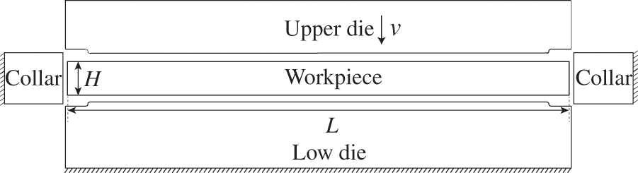
Figure 5: Schematic diagram of the imprinting model. The upper die moves down with a constant velocity of ν=6 m/s. The lower die and collar stay stationary

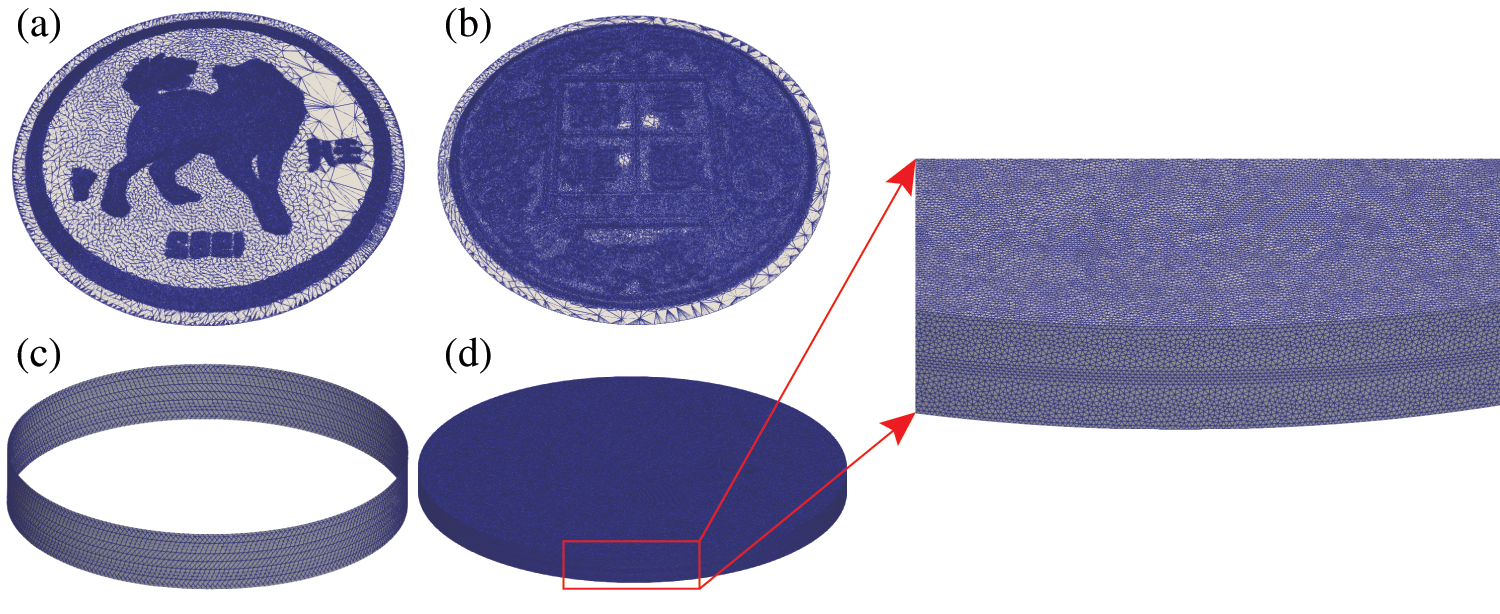
Figure 6: The zodiac dog finite element model of imprint forming. Discretizations of the upper die (a), the lower die (b), the collar (c), and the initial workpiece (d)

σy=(A+Bε¯nh)(26)

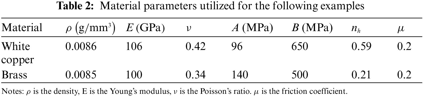
where σy represents the effective stress, ε¯ denotes the effective plastic strain. A and B are the initial yield stress and strength coefficient, respectively. nh is the hardening index.

Fig. 7 presents the results of this simulation example, where panels (a) and (b) show the stress of the coin obtained by using CoinFEM, while panels (c) and (d) display the deformed coin after being subjected to a 100-ton press force in an experimental setting. The black color observed in panels (c) and (d) is a consequence of mirror reflection in the flat area. However, if the black color appears in the regions of reliefs, it signifies insufficient filling of cavities in those areas. As illustrated in panel (a), the simulated stresses of region A are relatively small. This is caused by the fact that the reliefs in region A are the highest. Thus, the cavities would be filled at the last stage of the coining process. In this example, there is not enough material to fill the highest cavities sufficiently that both are captured by CoinFEM (see region A of the panel (a)) and the experiment (see region D of the panel (c)). Similarly, other insufficient regions also are found by the numerical and experiment methods (see region B of panel (a) and C of panel (B)) and the experiment (see region E of panel (c) and region F of panel (d)).

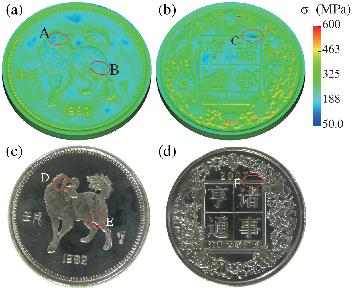
Figure 7: Numerical and experimental simulation results with embossing force of 100 tons. Predicted stress distributions on the positive side (a) and negative side (b) deformed positive side (c) and negative side (d) by experiment

4.2 Chinese Zodiac Cow Commemorative Coin

Fig. 8 illustrates the finite element model used for the zodiac cow commemorative coin, comprising of the upper die, lower die, collar, and workpiece. During the process, the upper die moves downwards with a constant velocity of ν=6 m/s, while the lower die and collar remain stationary. The stroke of the upper die is set to 0.6 mm. The workpiece is created by extruding a height of 2 mm through a square, which is discretized into 6.53 million tetrahedral meshes. The upper die, lower die, and collar are discretized into 244936, 244875, and 4656 triangular elements, respectively. The material of the workpiece is brass, and its parameters are shown in Table 2.

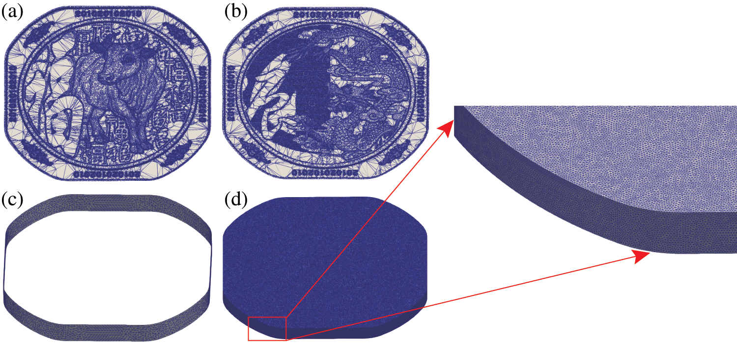
Figure 8: The zodiac cow finite element model of imprint forming. Discretizations of the upper die (a), the lower die (b), the collar (c), and the initial workpiece (d)

To evaluate the case of the Chinese zodiac cow commemorative coin, simulations are conducted using pure MPI, pure OpenMP, and hybrid MPI/OpenMP parallel solvers, and their findings are compared with the results obtained by the serial solver, whose performance was validated in our previous publications [1,19,34,35]. The comparison of the forming forces obtained from the three solvers is presented in Fig. 9. The serial curve in the figure is used as a reference, which shows an overall upward trend as the stroke of the upper die increases, reaching a maximum value of 11.0×105 N at a stroke of 0.14 mm. Curves of forming forces over the stroke are then plotted in the cases of parallel calculations. As we can see, the curves of pure MPI, pure OpenMP, and hybrid MPI/OpenMP closely coincide with the serial one. The maximum relative error of the forming forces between the parallel solvers and serial solvers is about 0.3%, thereby verifying the correctness of the parallel codes.

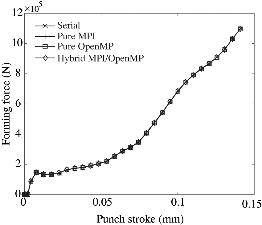
Figure 9: Comparison of curves of forming forces predicted by the serial, pure MPI, pure OpenMP, and hybrid MPI/OpenMP solvers

The stress-strain and Z-displacement distributions from the four solvers are presented in Fig. 10. The panels (a)–(d) in the first row display the results of effective stress for the serial, pure MPI, pure OpenMP, and hybrid MPI/OpenMP solvers, respectively. Meanwhile, panels (e)–(h) in the second row depict the effective plastic strain obtained from the four solvers, respectively. The third row, represented by panels (i)–(l), illustrates the corresponding displacement in the Z-direction.

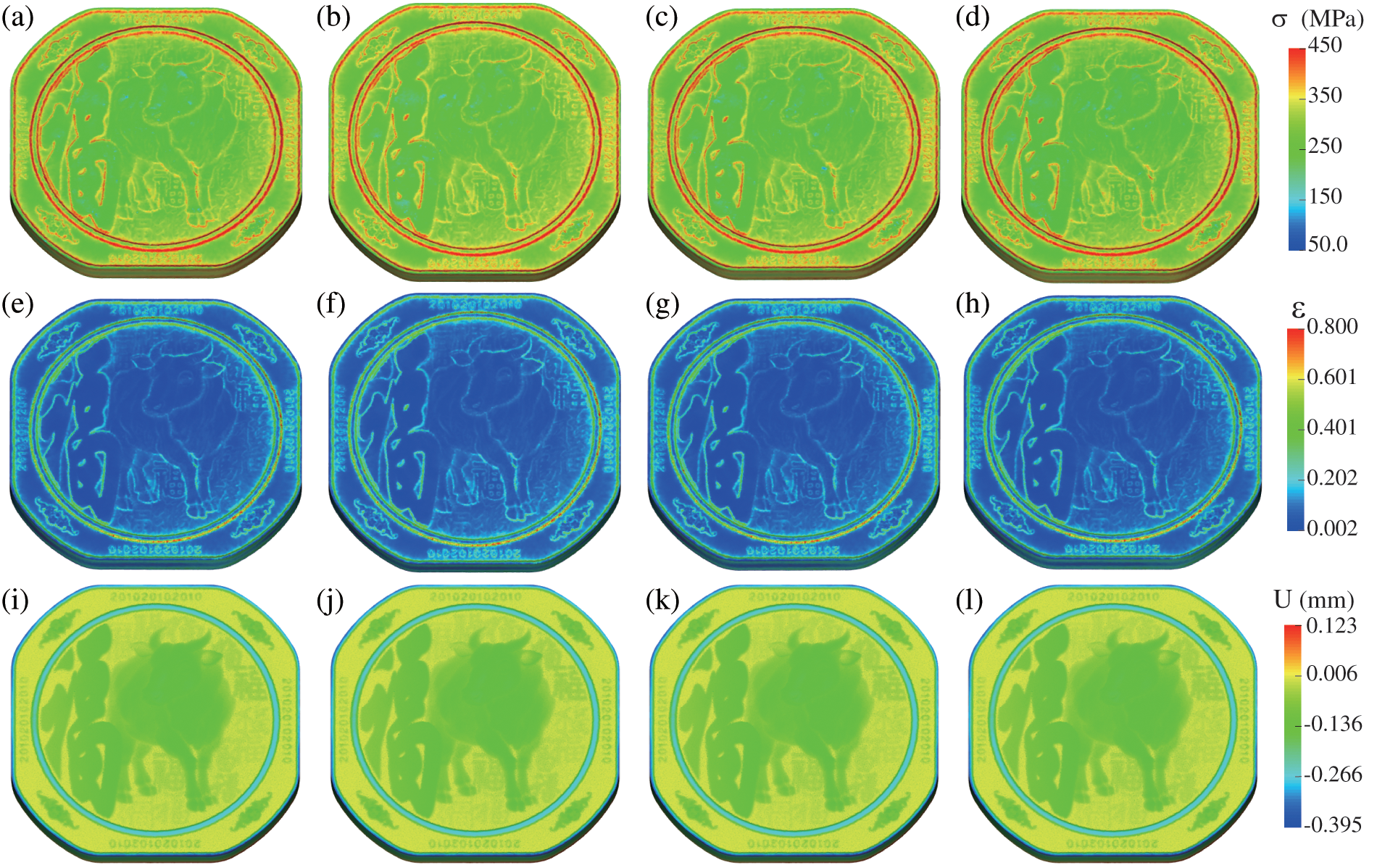
Figure 10: Effective stresses of the serial (a), pure MPI (b), pure OpenMP (c), and hybrid MPI/OpenMP (d), solvers. Effective strains of the serial (e), pure MPI (f), pure OpenMP (g), and hybrid MPI/OpenMP (h) solvers. Displacement in the Z-direction of the serial (i), pure MPI (j), pure OpenMP (k), and hybrid MPI/OpenMP (l) solvers

Contour plots illustrating the differences in Z-displacements obtained through three parallel solving methods, as compared to the serial results, are presented in Fig. 11. The plots in the first row, panels (a)–(c), depict the displacement differences on the positive side, while panels (e)–(h) in the second row illustrate the differences on the negative side. These subplots clearly show that the three solvers produce almost the same effective stresses and strains. Once again, the correctness of the parallel solvers is verified.

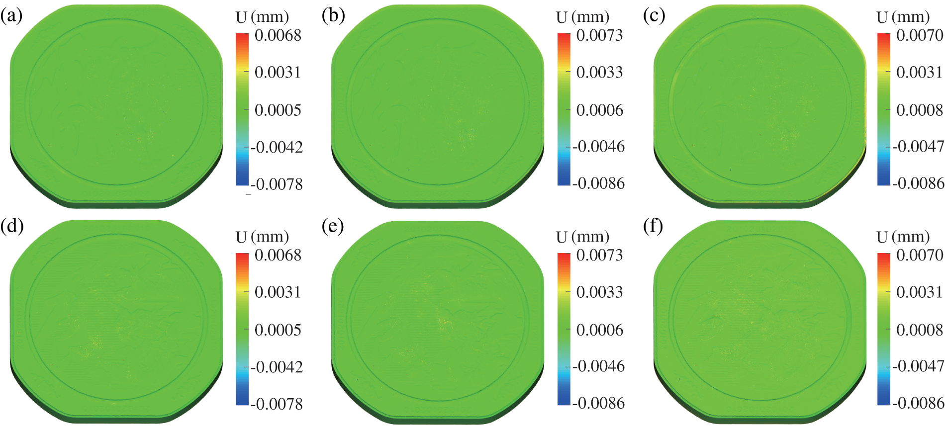
Figure 11: Displacement differences of the pure MPI (a), pure OpenMP (b), and hybrid MPI/OpenMP (c) solvers on the positive side of the coin. Displacement differences of the pure MPI (d), pure OpenMP (e), and hybrid MPI/OpenMP (f) solvers on the negative side of the coin

The quality of a parallel algorithm is typically measured by its speedup ratio Sp and parallel efficiency ep [36] which are defined as follows:

Sp=TsTp,ep=SpNc(27)

where Ts is the CPU time taken by a serial program to solve the problem on a single core; Tp is the computational time from multiple cores (or threads) to solve the same problem by parallel solver; Nc is the number of cores (or threads) used for the calculation.

All the above simulations in this example are carried out by an Intel i7-10700 processor with 8 cores and 16 threads (named Computer 1), and an Intel Xeon Silver 4310 processor with 12 cores and 24 threads (named Computer 2). The computational CPU times over cores/threads obtained by the two parallel solvers with the two different computers are plotted in Fig. 12. With the increasing of cores/threads, all CPU times in panels (a) and (b) tend to decrease faster initially, and then converge to a steady computational time even with the maximum cores/threads adopted. According to Eq. (27), the performances of pure MPI and pure OpenMP on two computers are compared, as shown in Fig. 13.

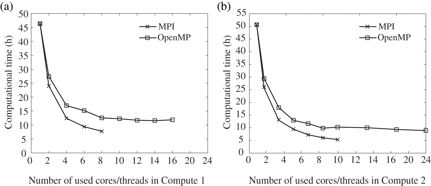
Figure 12: The CPU times consumed by MPI and OpenMP parallel solvers with Computer 1 (a), and Computer 2 (b)

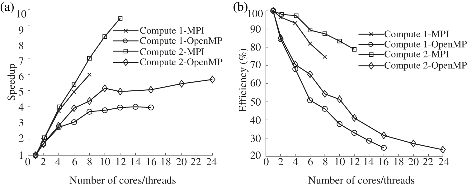
Figure 13: Comparison of speedup ratio (a) and parallel efficiency (b) of two different computers

According to Fig. 13, we can observe the influence of different computer performances on the serial/parallel solvers. When the same solver is adopted to solve the same example in serial mode, the time required by Computer 1 is 10%–15% less than that of Computer 2 (detailed CPU calculation times in serial cases are not listed). In parallel mode, the parallel performance of Computer 2 is always better than that of Computer 1 regardless of which parallel scheme is used. In panel (a) of Fig. 13, the speedup ratios of the two computers in MPI mode are both better than those in OpenMP mode. Moreover, the Computer 2 processor performs better than the Computer 1 processor in both parallel modes. We also notice that the parallel efficiency of MPI illustrated in panel (b) is less than 100%. This is due to the communication time between different cores and the uneven distribution of calculation load among cores. In the case of OpenMP, the main reason for parallel efficiency less than 100% is the occurrence of data races between different threads.

4.3 Testing of Hybrid MPI/OpenMP Solver

For testing the hybrid parallel solver, we utilize the Tianhe-2 cluster, which offers high-performance computing capability. The compute nodes in this cluster are equipped with Intel Xeon E5-2692 CPUs, each containing 24 threads.

In this cluster, we have implemented the hybrid solver for both the Chinese zodiac dog commemorative coin (referred to as Example 1) discussed in Section 4.1, and the Chinese zodiac cow commemorative coin (referred to as Example 2) examined in Section 4.2. Since the correctness of the parallel solver has already been verified in the previous section, we will now focus on showcasing the parallel efficiency of the hybrid solver. Fig. 14 presents the acceleration ratio and parallel efficiency achieved by Example 1 and Example 2 using the hybrid MPI/OpenMP parallel solver in the cluster.

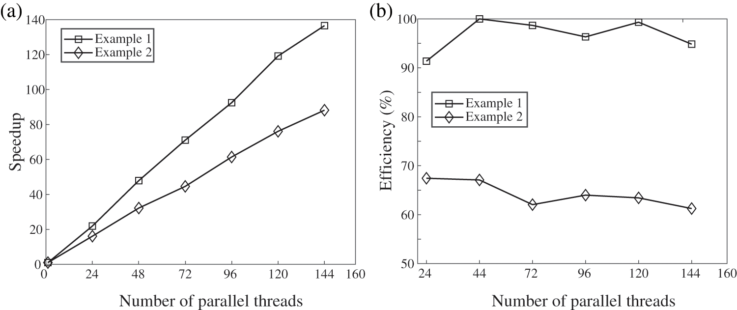
Figure 14: Comparison of speedup ratio (a) and parallel efficiency (b) of two examples in the cluster

Based on the observations from Fig. 14, it is evident that the speedup ratio of the hybrid MPI/OpenMP parallel solver exhibits a linear increase, while the parallel efficiency fluctuates within a specific range. These results indicate that the hybrid MPI/OpenMP parallel solver possesses favorable scalability. Notably, Example 1 achieves a maximum acceleration ratio of 136 when utilizing 144 parallel cores, further highlighting the effectiveness of the hybrid MPI/OpenMP approach. Furthermore, from Fig. 14, we can also observe that the acceleration effect of Example 1 is better than that of Example 2, mainly for two reasons. First, because the partitioning method used for parallel regions in the text cannot achieve complete load balance in a meaningful sense, the symmetry of the physical structure of Example 1 is better than that of Example 2, resulting in better performance of the former’s partitions. Second, the number of tetrahedral elements in Example 1 is 7.46 million, while in Example 2, it is 6.53 million. Thus, the former case requires more computational power, leading to better parallel performance.

5  Conclusions

The goal of this study is to address the challenge of prolonged simulation times associated with the intricate relief patterns found in traditional serial programs for commemorative coins. To tackle this issue, we parallelize a dynamic explicit finite element solver designed for simulating commemorative coins within both a single computer and a computer cluster environment. We develop parallel algorithm solvers utilizing pure MPI, pure OpenMP, and hybrid MPI/OpenMP approaches to replicate the coining process. Implementation examples are carried out on a single computer with multiple cores/threads using pure MPI and pure OpenMP parallel environments. Additionally, simulations are also performed on the Tianhe-2 cluster with multiple cores using hybrid MPI/OpenMP environments. This research focuses on addressing the following five key points:

•   The CoinFEM programs for commemorative coining simulation incorporate three parallel schemes: pure MPI, pure OpenMP, and hybrid MPI/OpenMP, to enhance its performance. The correctness of the parallel solvers is verified by comparing the obtained results with the serial results and experimental data using the same finite element model.

•   During testing on a single computer environment, the pure MPI and pure OpenMP parallel solvers exhibit notable speedup ratios. Specifically, on the Intel i7-10700 hardware configuration, the pure MPI parallel solver achieves a speedup ratio of 6, while the pure OpenMP parallel solver achieves a speedup ratio of 3.5. On the other hand, when utilizing the Intel Xeon Silver 4310 hardware configuration, the pure MPI parallel solver achieves a speedup ratio of 9.5, while the pure OpenMP parallel solver achieves a speedup ratio of 5.7. These results demonstrate the effectiveness of both pure MPI and pure OpenMP parallelization techniques in improving computational efficiency on different hardware configurations.

•   When employing the hybrid MPI/OpenMP parallel solver for testing purposes in clusters, remarkable acceleration ratios are achieved for the two examples. Specifically, Example 1 achieves an acceleration ratio of 136, while Example 2 achieves an acceleration ratio of 88. These significant acceleration ratios demonstrate the capability of the hybrid MPI/OpenMP parallel solver to meet the simulation requirements for accurately capturing intricate relief patterns on commemorative coins.

•   The pure MPI parallel algorithm is highly suitable for parallelizing the dynamic explicit codes of the imprint forming solver, leading to reduced resource wastage and improved computing efficiency, especially on a single computer. In comparison, the pure OpenMP parallel algorithm may not provide the same level of efficiency. The hybrid MPI/OpenMP parallel algorithms exhibit a fluctuating parallel efficiency within a certain range, while the acceleration ratio shows a consistent linear improvement. These results provide evidence of the good scalability and effectiveness of the parallel algorithm.

Acknowledgement: We thank anonymous reviewers and journal editors for assistance. We also appreciate the financial assistance provided by the funding agencies.

Funding Statement: This work was supported by the fund from Shenyang Mint Company Limited (No. 20220056), Senior Talent Foundation of Jiangsu University (No. 19JDG022) and Taizhou City Double Innovation and Entrepreneurship Talent Program (No. Taizhou Human Resources Office [2022] No. 22).

Author Contributions: YL (Yang Li) performed all of the modelings, collected the research literature and wrote the draft. JX was responsible for organizing and finalizing the paper. YL (Yun Liu) performed simulations and made figures. WZ and FW provided experiment data and suggestions. All the authors discussed the results and contributed to the final paper.

Availability of Data and Materials: All data included in this study are available upon request by contacting the corresponding author.

Conflicts of Interest: The authors declare that they have no known competing financial interests or personal relationships that could have appeared to influence the work reported in this paper. The authors also declare that they do not have any financial interests/personal relationships, which may be considered as potential competing interests.

References

1. Xu, J., Liu, Y., Li, S., Wu, S. (2008). Fast analysis system for embossing process simulation of commemorative coin-coinform. Computer Modeling in Engineering & Sciences, 38(3), 201–215. https://doi.org/10.3970/cmes.2008.038.201 [Google Scholar] [CrossRef]

2. Zhong, W., Liu, Y., Hu, Y., Li, S., Lai, M. (2012). Research on the mechanism of flash line defect in coining. The International Journal of Advanced Manufacturing Technology, 63, 939–953. https://doi.org/10.1007/s00170-012-3952-3 [Google Scholar] [CrossRef]

3. Li, Q., Zhong, W., Liu, Y., Zhang, Z. (2017). A new locking-free hexahedral element with adaptive subdivision for explicit coining simulation. International Journal of Mechanical Sciences, 128, 105–115. https://doi.org/10.1016/j.ijmecsci.2017.04.017 [Google Scholar] [CrossRef]

4. Alexandrino, P., Leitão, P. J., Alves, L. M., Martins, P. (2018). Finite element design procedure for correcting the coining die profiles. Manufacturing Review, 5, 3. https://doi.org/10.1051/mfreview/2018007 [Google Scholar] [CrossRef]

5. Alexandrino, P., Leitão, P. J., Alves, L. M., Martins, P. (2017). Numerical and experimental analysis of coin minting. Proceedings of the Institution of Mechanical Engineers, Part L: Journal of Materials: Design and Applications, 233(5), 842–849. https://doi.org/10.1177/1464420717709833 [Google Scholar] [CrossRef]

6. Afonso, R. M., Alexandrino, P., Silva, F. M., Leitão, P. J., Alves, L. M. et al. (2019). A new type of bi-material coin. Proceedings of the Institution of Mechanical Engineers, Part B: Journal of Engineering Manufacture, 233(12), 2358–2367. https://doi.org/10.1177/0954405419840566 [Google Scholar] [CrossRef]

7. Peng, Y., Xu, J., Wang, Y. (2022). Predictions of stress distribution and material flow in coining process for bi-material commemorative coin. Materials Research Express, 9(6), 066505. https://doi.org/10.1088/2053-1591/ac7515 [Google Scholar] [CrossRef]

8. Bova, S. W., Breshears, C. P., Gabb, H., Kuhn, B., Magro, B. et al. (2001). Parallel programming with message passing and directives. Computing in Science and Engineering, 3(5), 22–37. https://doi.org/10.1109/5992.947105 [Google Scholar] [CrossRef]

9. Witkowski, T., Ling, S., Praetorius, S., Voigt, A. (2015). Software concepts and numerical algorithms for a scalable adaptive parallel finite element method. Advances in Computational Mathematics, vol. 41, pp. 1145–1177. https://doi.org/10.1007/s10444-015-9405-4 [Google Scholar] [CrossRef]

10. Gabriel, E., Fagg, G. E., Bosilca, G., Angskun, T., Dongarra, J. J. et al. (2004). Open MPI: Goals, concept, and design of a next generation MPI implementation. In: Lecture notes in computer science, vol. 3241, pp. 97–104. Budapest, Hungary. https://doi.org/10.1007/978-3-540-30218-6_19 [Google Scholar] [CrossRef]

11. Devietti, J., Lucia, B., Ceze, L., Oskin, M. (2010). DMP: Deterministic shared-memory multiprocessing. Institute of Electrical and Electronics Engineers Micro, 30(1), 40–49. https://doi.org/10.1109/MM.2010.14 [Google Scholar] [CrossRef]

12. Dagum, L., Menon, R. (1998). OpenMP: An industry standard API for shared-memory programming. Institute of Electrical and Electronics Engineers Computational Science and Engineering, 5(1), 46–55. https://doi.org/10.1109/99.660313 [Google Scholar] [CrossRef]

13. Sato, M. (2002). OpenMP: Parallel programming API for shared memory multiprocessors and on-chip multiprocessors. Proceedings of the 15th International Symposium on System Synthesis, pp. 109–111. Kyoto, Japan. https://doi.org/10.1145/581199.581224 [Google Scholar] [CrossRef]

14. Pantalé, O. (2005). Parallelization of an object-oriented FEM dynamics code: Influence of the strategies on the speedup. Advances in Engineering Software, 36(6), 361–373. https://doi.org/10.1016/j.advengsoft.2005.01.003 [Google Scholar] [CrossRef]

15. Fialko, S. (2021). Parallel finite element solver for multi-core computers with shared memory. Computers and Mathematics with Applications, 94, 1–14. https://doi.org/10.1016/j.camwa.2021.04.013 [Google Scholar] [CrossRef]

16. Jin, H., Jespersen, D., Mehrotra, P., Biswas, R., Huang, L. et al. (2011). High performance computing using MPI and OpenMP on multi-core parallel systems. Parallel Computing, 37(9), 562–575. https://doi.org/10.1016/j.parco.2011.02.002 [Google Scholar] [CrossRef]

17. Song, K., Liu, P., Liu, D. (2021). Implementing delay multiply and sum beamformer on a hybrid CPU-GPU platform for medical ultrasound imaging using OpenMP and CUDA. Computer Modeling in Engineering & Sciences, 128(3), 1133–1150. https://doi.org/10.32604/cmes.2021.016008 [Google Scholar] [CrossRef]

18. Khaleghzadeh, H., Fahad, M., Shahid, A., Manumachu, R. R., Lastovetsky, A. (2020). Bi-objective optimization of data-parallel applications on heterogeneous HPC platforms for performance and energy through workload distribution. IEEE Transactions on Parallel and Distributed Systems, 32(3), 543–560. https://doi.org/10.1109/TPDS.2020.3027338 [Google Scholar] [CrossRef]

19. Xu, J., Chen, X., Zhong, W., Wang, F., Zhang, X. (2021). An improved material point method for coining simulation. International Journal of Mechanical Sciences, 196, 106258. https://doi.org/10.1016/j.ijmecsci.2020.106258 [Google Scholar] [CrossRef]

20. Kawka, M., Olejnik, L., Rosochowski, A., Sunaga, H., Makinouchi, A. (2001). Simulation of wrinkling in sheet metal forming. Journal of Materials Processing Technology, 109(3), 283–289. https://doi.org/10.1016/S0924-0136(00)00813-X [Google Scholar] [CrossRef]

21. Browne, S., Dongarra, J., Garner, N., Ho, G., Mucci, P. (2000). A portable programming interface for performance evaluation on modern processors. The International Journal of High Performance Computing Applications, 14(3), 189–204. https://doi.org/10.1177/109434200001400303 [Google Scholar] [CrossRef]

22. Nielsen, F. (2016). Introduction to MPI: The message passing interface. In: Introduction to HPC with MPI for data science, pp. 21–62. Switzerland: Springer Cham. https://doi.org/10.1007/978-3-319-21903-5_2 [Google Scholar] [CrossRef]

23. Sairabanu, J., Babu, M., Kar, A., Basu, A. (2016). A survey of performance analysis tools for OpenMP and MPI. Indian Journal of Science and Technology, 9(43), 1–7. https://doi.org/10.17485/ijst/2016/v9i43/91712 [Google Scholar] [CrossRef]

24. Zhang, R., Xiao, L., Yan, B., Wei, B., Zhou, Y. et al. (2019). A source code analysis method with parallel acceleration for mining MPI application communication counts. 2019 IEEE 21st International Conference on High Performance Computing and Communications, Zhangjiajie, China. https://doi.org/10.1109/HPCC/SmartCity/DSS.2019.00034 [Google Scholar] [CrossRef]

25. Oh, S. E., Hong, J. W. (2017). Parallelization of a finite element fortran code using OpenMP library. Advances in Engineering Software, 104, 28–37. https://doi.org/10.1016/j.advengsoft.2016.11.004 [Google Scholar] [CrossRef]

26. Ayub, M. A., Onik, Z. A., Smith, S. (2019). Parallelized RSA algorithm: An analysis with performance evaluation using OpenMP library in high performance computing environment. 2019 22nd International Conference on Computer and Information Technology (ICCIT), Dhaka, Bangladesh. https://doi.org/10.1109/ICCIT48885.2019.9038275 [Google Scholar] [CrossRef]

27. Sefidgar, S. M. H., Firoozjaee, A. R., Dehestani, M. (2021). Parallelization of torsion finite element code using compressed stiffness matrix algorithm. Engineering with Computers, 37, 2439–2455. https://doi.org/10.1007/s00366-020-00952-w [Google Scholar] [CrossRef]

28. Zhang, H., Liu, Y., Liu, L., Lai, X., Liu, Q. et al. (2022). Implementation of OpenMP parallelization of rate-dependent ceramic peridynamic model. Computer Modeling in Engineering & Sciences, 133(1), 195–217. https://doi.org/10.32604/cmes.2022.020495 [Google Scholar] [CrossRef]

29. Atzeni, S., Gopalakrishnan, G., Rakamaric, Z., Ahn, D. H., Laguna, I. et al. (2016). ARCHER: Effectively spotting data races in large OpenMP applications. 2016 Institute of Electrical and Electronics Engineers International Parallel and Distributed Processing Symposium (IPDPS), pp. 53–62. Chicago, IL, USA, Institute of Electrical and Electronics Engineers. https://doi.org/10.1109/IPDPS.2016.68 [Google Scholar] [CrossRef]

30. Sziveri, J., Seale, C., Topping, B. H. V. (2000). An enhanced parallel sub-domain generation method for mesh partitioning in parallel finite element analysis. International Journal for Numerical Methods in Engineering, 47(10), 1773–1800. [Google Scholar]

31. Jiao, Y. Y., Zhao, Q., Wang, L., Huang, G. H., Tan, F. (2019). A hybrid MPI/OpenMP parallel computing model for spherical discontinuous deformation analysis. Computers and Geotechnics, 106, 217–227. https://doi.org/10.1016/j.compgeo.2018.11.004 [Google Scholar] [CrossRef]

32. Guo, X., Lange, M., Gorman, G., Mitchell, L., Weiland, M. (2015). Developing a scalable hybrid MPI/OpenMP unstructured finite element model. Computers & Fluids, 110, 227–234. https://doi.org/10.1016/j.compfluid.2014.09.007 [Google Scholar] [CrossRef]

33. Velarde Martínez, A. (2022). Parallelization of array method with hybrid programming: OpenMP and MPI. Applied Sciences, 12(15), 7706. https://doi.org/10.3390/app12157706 [Google Scholar] [CrossRef]

34. Xu, J., Khan, K., El Sayed, T. (2013). A novel method to alleviate flash-line defects in coining process. Precision Engineering, 37(2), 389–398. https://doi.org/10.1016/j.precisioneng.2012.11.001 [Google Scholar] [CrossRef]

35. Li, J., Yan, T., Wang, Q., Xu, J., Wang, F. (2023). Isogeometric analysis based investigation on material filling of coin cavities. AIP Advances, 13(3), 035311. https://doi.org/10.1063/5.0139826 [Google Scholar] [CrossRef]

36. Jarzebski, P., Wisniewski, K., Taylor, R. L. (2015). On parallelization of the loop over elements in FEAP. Computational Mechanics, 56(1), 77–86. https://doi.org/10.1007/s00466-015-1156-z [Google Scholar] [CrossRef]