The Lambert-G Family: Properties, Inference, and Applications

1  Introduction

Many approaches have been suggested to propose new families of distributions or to generalize some of the classical distributions. These families and generalized distributions provide more flexibility in modeling real-life data in different applied fields. The most common feature of the new families and generalized distributions is represented by having one or more extra shape parameters. Hence, the statistical literature contains many families to generate new distributions by adding one or more shape parameters. Some examples include the Kumaraswamy-G by Cordeiro et al. [1], exponentiated T-X by Alzaghal et al. [2], Weibull-G by Bourguignon et al. [3], odd moment exponential-G by Haq et al. [4], Burr XII-G by Cordeiro et al. [5], generalized odd Burr III-G by Haq et al. [6], generalized odd half-logistic-G by Altun et al. [7], Marshall–Olkin alpha power by Nassar et al. [8], new exponential-X by Ahmad et al. [9], new extended heavy-tailed family by Aljohani et al. [10], and modified generalized-G by Shama et al. [11].

One of the most notable approaches to generating new distributions is constructed by using the Lambert-W (LW) function which is also known as the product logarithm function. This approach is discussed by Corless [12]. It is defined (for z∈[0,∞)) as the roots of the following function:

W(z)eW(z)=z;z∈C.(1)

The above equation contains only one real-valued solution. Recently, the LW function has been used in the distribution of prime numbers as discussed by Visser [13]. Goerg [14] adopted the LW function to introduce new families of distributions in the context of random variable transformations. Iriarte et al. [15] generated the Lambert-F class as an alternative family for positive data analysis.

This study introduces a new wider class based on the LW function called the Lambert-G (LG) family, in which the baseline distribution is a continuous distribution with positive support. The proposed approach applies a transformation to a baseline cumulative distribution function (cdf), as illustrated in Definition 1. The newly generated cdf of the LG family, with two extra shape parameters, has the quantile function (qf), which is expressed in a closed form in terms of the LW function; hence, the proposed generator is called the LG family.

The LG family has some desirable properties and it can be justified as follows. (i) The three-parameter special sub-models of the LG family are capable of modeling all important hazard rate (hr) shapes including increasing, decreasing, unimodal, J-shape, reversed J-shape, bathtub, and modified-bathtub failure rates; (ii) Moreover, the densities of its sub-models accommodate reversed J shaped, right-skewed, symmetric, left-skewed, decreasing-increasing-decreasing densities; (iii) The LG special sub-models generalize some well-known distributions in the distribution theory literature such as the modified Weibull model [16]; (iv) The LG special models provide better fit than other generalized models under the same baseline distribution as shown in case of the Lambert-Lomax (LL) model.

The paper is organized in the following sections. In Section 2, the LG family is presented. In Section 3, we provide three special sub-models of the LG family. The properties of the LL distribution along with its analytical shapes are explored in Section 4. In Section 5, the parameters of the LL distribution are estimated via six classical estimation methods. Section 6 presents simulation results to address the behavior of different estimators. To show the empirical importance of the LL distribution, two real-life data sets are analyzed in Section 7. Final remarks are given in Section 8.

2  The LG Family

Definition 1. A random variable X is said to follow the LG family, denoted by X∽LG (x;υ,ω,ξ), if its cdf is given by

F(x;υ,ω,ξ)=1−exp⁡(−{−ln⁡[G¯(x;ξ)]}υexp⁡{−ωln⁡[G¯(x;ξ)]}),x>0,υ,ω,ξ>0,(2)

where υ and ω are additional shape parameters and G¯(x;ξ) is a baseline survival function (sf) with a vector of unknown parameters ξ.

The probability density function (pdf) corresponding to Eq. (2) reduces to

f(x;υ,ω,ξ)={υ−ωln⁡[G¯(x;ξ)]}h(x;ξ){−ln⁡[G¯(x;ξ)]}1−υexp⁡{−ωln⁡[G¯(x;ξ)]}F¯(x;υ,ω,ξ),(3)

where F¯(x;υ,ω,ξ) is the sf of the LG family and h(x;ξ) is the hr function (hrf) of a baseline distribution.

The hrf of the LG family becomes

φ(x;υ,ω,ξ)={υ−ωln⁡(G¯(x;ξ))}h(x;ξ){−ln⁡[G¯(x;ξ)]}υ−1exp⁡{−ωln⁡[G¯(x;ξ)]}.(4)

According to Eq. (4), the hrf of the LG family has a flexible property because it depends on the value of the extra parameter υ and the baseline hrf. Furthermore, the importance of the proposed family follows from its ability to generate new flexible distributions without adding new extra parameters by letting υ=ω=1 in Eq. (2). Then, Eq. (2) reduces to

F(x;ξ)=1−exp⁡{−G¯(x;ξ)ln⁡[G¯(x;ξ)]}=1−[G¯(x;ξ)]1G¯(x;ξ).(5)

Eq. (5) is called the reduced Lambert-G (RLG) family.

The pdf and hrf of the RLG are given, respectively, by

f(x;ξ)=h(x;ξ){1−ln⁡[G¯(x;ξ)]}[G¯(x;ξ)]−F¯(x;ξ)(6)

and

φ(x;ξ)=h(x;ξ)1−ln⁡[G¯(x;ξ)]G¯(x;ξ).(7)

3  Special Models of the LG Family

In this section, we provide three specific models of the LG family. These special distributions provide modified flexible forms of some standard distributions namely the exponential, Pareto, and Lomax distributions. The special sub-models of the LG family are called the Lambert-exponential (LE), Lambert-Pareto (LP), and LL distributions. These special models are capable of modeling all important hrf shapes including increasing, decreasing, unimodal, J-shape, reversed J-shape, bathtub, and modified bathtub failure rates. Moreover, the densities of these sub-models can also provide reversed J-shaped, right-skewed, symmetric, left-skewed, decreasing-increasing-decreasing densities.

3.1 The LE Distribution

The LE cdf follows from Eq. (2) by setting G¯(x;θ)=exp⁡(−θx). Then, the LE cdf becomes

F(x;υ,α,λ)=1−exp⁡(−αxυeλx),x>0,υ,α,λ>0,(8)

where α=θυ and λ=ωθ are scale parameters and υ is a shape parameter.

The corresponding pdf and hrf of the LE distribution take the forms

f(x;υ,α,λ)=α[υ+λx]xυ−1exp⁡(λx−αxυeλx)(9)

and

φ(x;υ,α,λ)=α[υ+λx]xυ−1exp⁡(λx).(10)

The hrf shapes of the LE distribution depend only on the value of υ and can be increasing or bathtub shaped. The LE distribution is also known in the literature as the modified Weibull distribution (see Lai et al. [16]). Hence, the LE model reduces to type I extreme-value distribution for υ=0 and reduces to the Weibull distribution for λ=0.

3.2 The LP Distribution

Consider the sf of the Pareto distribution G¯(x;α)=(1/x)α, x≥1 and α>0. Substituting G¯(x;α)=(1/x)α in (2) yields the cdf of the LP distribution

F(x;υ,λ,β)=1−exp⁡(−λxβ[ln⁡(x)]υ),x>1,υ,λ,β>0,(11)

where λ=αυ is a scale parameters and β=ωα and υ are shape parameters. The corresponding pdf and hrf are given by

f(x;υ,λ,β)=λ[υ+βln⁡(x)]xβ−1[ln⁡(x)]υ−1exp⁡(−λxβ[ln⁡(x)]υ)(12)

and

φ(x;υ,λ,β)=λ[υ+βln⁡(x)]xβ−1[ln⁡(x)]υ−1.(13)

The shape of the LP hrf depends on the values of β and υ and it can provide increasing or bathtub shapes. The Weibull and Pareto distributions are special cases from the LP distribution. The Weibull distribution follows when υ=0 and the Pareto model is obtained for υ=1 and β=0. Fig. 1 provides some possible shapes of the density and hazard functions of the LE and LP distributions.

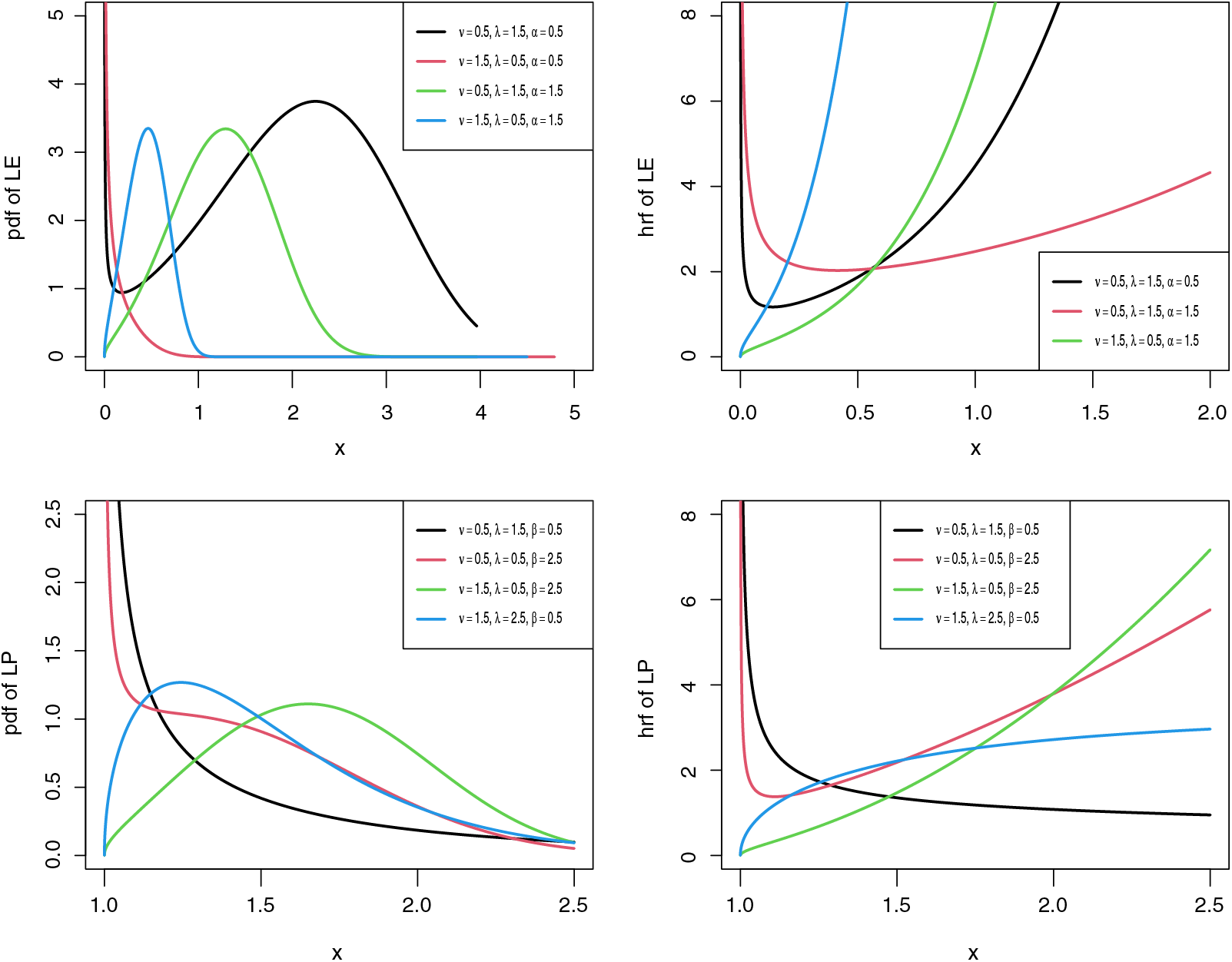
Figure 1: Possible shapes for the density and hazard functions of the LE and LP distributions

3.3 The LL Distribution

By taking the sf of the Lomax distribution, G¯(x;α)=(1+xα)−1, α>0, as a baseline sf in (2). The cdf of the LL distribution reduces to

F(x;υ,ω,α)=1−exp⁡{−(1+xα)ω[ln⁡(1+xα)]υ},x>0,υ,ω,α>0,(14)

where υ>0 and ω>0 are two extra shape parameters.

The corresponding pdf and hrf are

f(x;υ,ω,α)=1α[υ+ωln⁡(1+xα)](1+xα)ω−1[ln⁡(1+xα)]υ−1F¯(x;υ,ω,α)(15)

and

φ(x;υ,ω,α)=1α[υ+ωln⁡(1+xα)][1+xα]ω−1[ln⁡(1+xα)]υ−1.(16)

The Lomax distribution follows as a special case of the LL distribution with υ=1 and ω=0. The behavior of the LL density is plotted in Fig. 2. The hrf plots of the LL model are shown in Fig. 3. These figures show the strong effects of the two shape parameters ω and υ on the shapes of the pdf and hrf of the LL distribution.

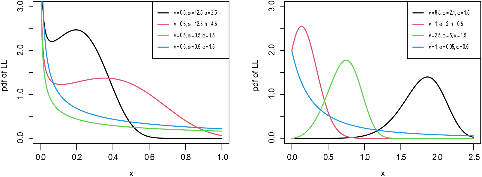
Figure 2: Possible shapes for the pdf of the LL distribution

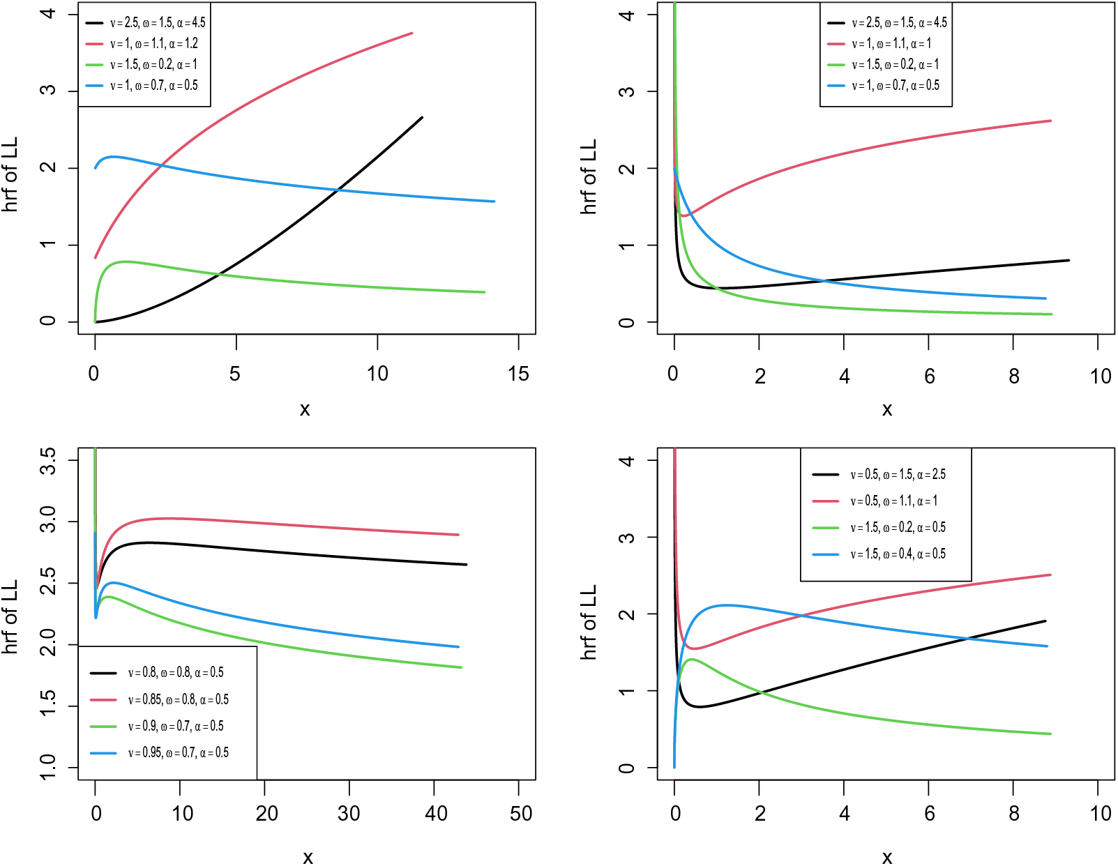
Figure 3: Possible shapes for the hrf of the LL distribution

4  Properties of the LL Distribution

In this section, we provide some basic statistical properties of the LL distribution.

4.1 Behavior of the Density and Hazard Rate Functions

The pdf limits of the LL distribution as x→0 and as x→∞ are

limx→0f(x;υ,ω,α)={∞υ<1,1/αυ=1,0υ>1andlimx→∞f(x;υ,ω,α)=0.

Theorem 4.1. The graph of the pdf of the LL distribution is log-concave if υ≥1 for all x.

Proof. Setting y=ln⁡(1+xα) in the LL pdf (15) and taking the logarithm, we have

ψ(y)=1α(υ+ωy)yυ−1exp((ω−1)y−yυeωy).

Differentiating twice concerning y, we have

ψ″(y)=−ω2(υ+ωy)2−(υ−1)(1+υyυeωy)y2.

Note that y=ln⁡(1+xα) implies that y>0. So, we can conclude that for all values of ω and υ≥1, ψ″(y)<0. Hence, the pdf of the LL distribution is log-concave for all x.

The hrf limits of the LL distribution as x→0 and as x→∞ are

limx→0φ(x;υ,ω,α)={∞υ<1,1/αυ=1,0υ>1andlimx→∞φ(x;υ,ω,α)={0ω<1,∞ω≥1.

Theorem 4.2. The hrf of the LL distribution is

•   Increasing for υ≥1 and ω≥1.

•   Decreasing for υ≤1 and ω<0.5 or for υ<1, 0.5<ω<1 and υ<4ω(1−ω).

•   Unimodal for υ≥1 and 0.5<ω<1.

•   Bathtub for υ<1 and ω≥1.

•   Decreasing-increasing-decreasing for υ<1, 0.5<ω<1 and υ≥4ω(1−ω).

Proof. From Eq. (16), we have

ln⁡[φ(x;υ,ω,α)]=−ln⁡(α)+ln⁡[υ+ωln⁡(1+xα)]+(ω−1)ln⁡[1+xα]+(υ−1)ln⁡[ln⁡(1+xα)].

The derivative of ln⁡[φ(x;υ,ω,α)] follows as

ddxln⁡[φ(x;υ,ω,α)]=Ψ(ln⁡(1+xα))x+α,

where

Ψ(y)=ω(ω−1)y2+υ(2ω−1)y+υ(υ−1),y>0,

where y=ln⁡(1+xα).

Clearly, both the hrf of the LL distribution and Ψ(y) have the same sign, hence the quantity Ψ(y) has the following cases:

Case 1: For ω=1, Ψ(y) reduces to y+υ−1=0, hence the hrf of the LL distribution is increasing in x if υ≥1. Also, if υ<1, the hrf is a bathtub shape with a minimum value at the point y1=1−υ since Ψ′(y1)>0.

Case 2: If υ=1, Ψ(y) reduce to Ψ(y)=ω(ω−1)y2+(2ω−1)y. Hence, the LL hrf is increasing in x for ω≥1. The LL hrf is decreasing in x for ω≤0.5. Moreover, the LL hrf is unimodal with maximum value at the point y1=2ω−1ω(ω−1) for 0.5<ω<1 since Ψ′(y1)<0.

Case 3: If υ>1 and ω>1, then Ψ(y) is positive. Hence, the LL hrf is increasing in x.

Case 4: If υ<1 and ω≤0.5, hence Ψ(y) is negative. Then, the LL hrf is decreasing in x.

To discuss other cases, we have to get two critical values of Ψ(y) which can be written as

y1=υ(1−2ω)−4υω(ω−1)+υ22ω(ω−1)

and

y2=υ(1−2ω)+υ[4ω(ω−1)+υ]2ω(ω−1).

Case 5: For υ>1 and ω<1, Ψ(y) has a critical value at the point y2 which changes the sign from positive to negative. Thus, the LL hrf is unimodal.

Case 6: The function Ψ(y) has two critical values y1 and y2 where the sign is negative on (0,y1)⋃(y2,∞) and positive on (y1,y2) if 4ω(1−ω)<υ<1 and 0.5<ω<1. Hence, the LL hrf is decreasing-increasing-decreasing. Additionally, for υ<4ω(1−ω), the sign is always negative, thus the LL hrf is decreasing.

Case 7: For υ<1 and ω>1, Ψ(y) has a critical value at the point y2 which changes the sign from negative to positive. Thus, the LL hrf is the bathtub.

4.2 Moments

Theorem 4.3. The rth raw moments of the LL distribution can be obtained as

E(Xr)=αr∑i=0r∑j=0∞(ri)ij(−1)r−iAk1,...,kjj!Γ(Sj+1).(17)

Proof. The rth raw moments of the LL distribution can be defined as

E(Xr)=∫0∞xrαf(x;υ,ω,α)dx.

Let Y=ln⁡(1+Xα), y>0, then E(Xr) becomes

E(Xr)=αr∫0∞(ey−1)r[υ+ωy]eωyyυ−1exp⁡(−yυeωy)dy.

By using the binomial and series expansions, the rth raw moments take the form

E(Xr)=αr∫0∞∑i=0r∑j=0∞(ri)ij(−1)r−ij![υ+ωy]eωyyj+υ−1exp⁡(−yυeωy)dy.

Let z=yυeωy, hence y in terms in z becomes y=∑k=1∞akzk/υ, where ak=(−1)k+1kj−2(ω/υ)k−1(k−1)!. Then, the above integral reduces to

E(Xr)=αr∫0∞∑i=0r∑j=0∞(ri)ij(−1)r−ij!(∑k=1∞akzk/υ)jexp⁡(−z)dz.(18)

Let (∑k=1∞akzk/υ)j=∑k1,...,kj=1∞Ak1,...,kjzSj, where Ak1,...,kj=ak1...akj and Sj=j1+...+jj. Hence, the integral in (18) gives

E(Xr)=αr∑i=0r∑j=0∞(ri)ij(−1)r−iAk1,...,kjj!∫0∞zSjexp⁡(−z)dz.

Finally, we have

E(Xr)=αr∑i=0r∑j=0∞(ri)ij(−1)r−iAk1,...,kjj!Γ(Sj+1),

which completes the proof.

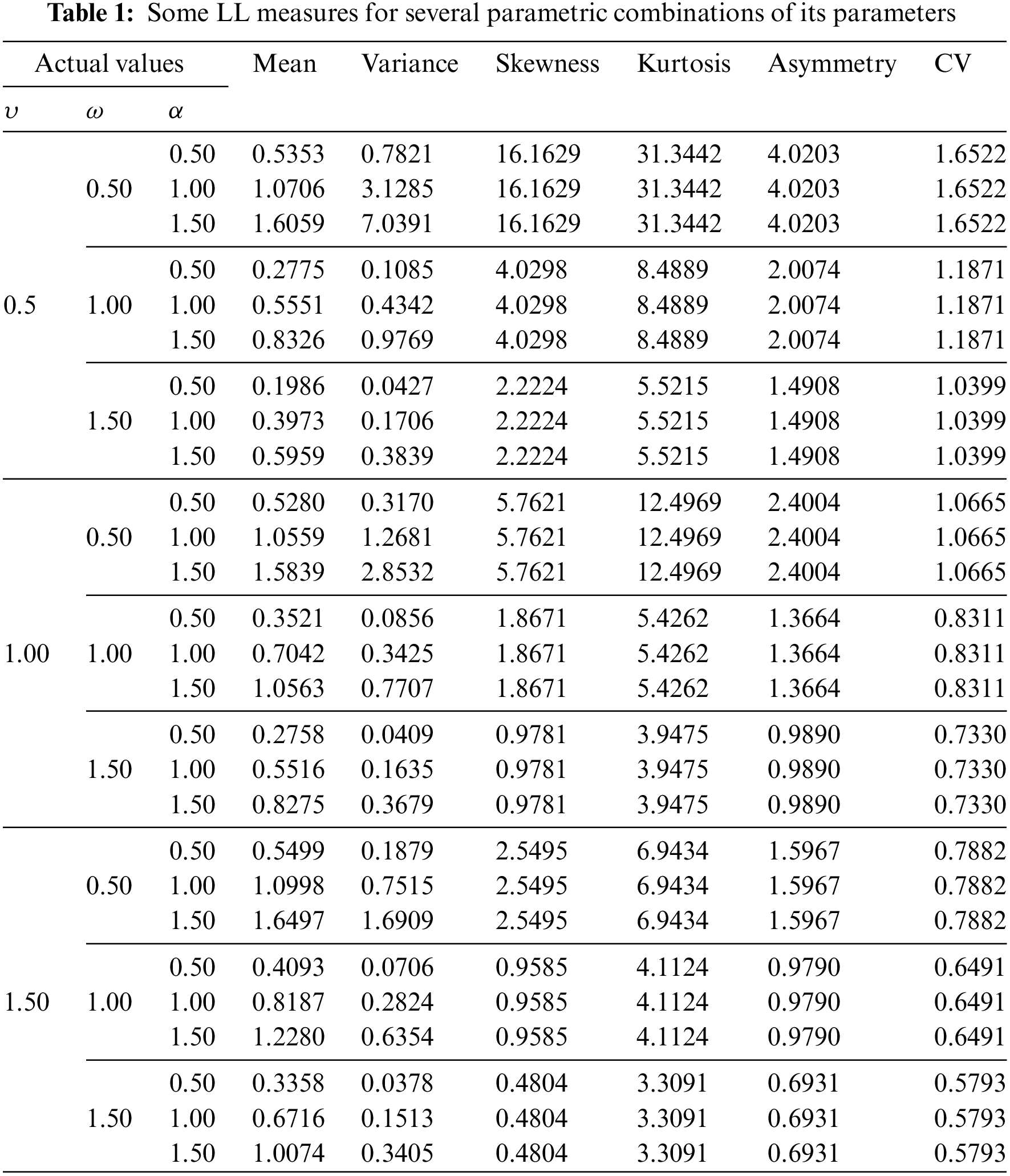
As well as the measures of skewness, kurtosis, and asymmetry of the LL distribution are obtained by the following relations:

β1=(μ3′−3μ2′μ+2μ3)2(μ2′−μ2)3,β2=μ4′−4μ3′μ+6μ2′μ2−3μ4(μ2′−μ2)2andβ3=μ3′−3μ2′μ+2μ3(μ2′−μ2)3/2.

Table 1 provides some important LL measures for various parametric values. The numerical values show that the LL distribution can be right skewed for different values of υ and ω.

4.3 Quantile Function

The qf of the LL distribution follows, by inverting its cdf (15), as

x=Q(u)=α{exp⁡[ek(u)]−1},(19)

where

k(u)=1υ({ln⁡[−ln⁡(1−u)]}−υW(ω[−ln⁡(1−u)]1/υυ))

and W(.) is the LW function. Then, if U has a uniform distribution in (0,1), the solution of nonlinear equation x=Q(u) has the LL distribution. Setting u=0.5 in (19) gives the median (M) of the LL distribution. Additionally, by setting u=0.25 and u=0.75, one can obtain the lower and higher quartiles, respectively. The qf is calculated by using the Maple software.

4.4 Order Statistics

The order statistic for the LL distribution will be discussed in this section. It will also be useful to derive the pdf of the kth order statistic X(k) of the ordered sample X(1),X(2),...,X(n) drawn from the LL with parameters υ, ω and α. The pdf fX(k)(x) of X(k) is given by

fX(k)(x)=n(n−1k−1)f(x)F(x)k−1[1−F(x)](n−k),k=1,2,...,n.(20)

We have

F(x;υ,ω,α)k−1=(1−e−(1+xα)ω[ln⁡(1+xα)]υ)k−1=∑l=0k−1(k−1l)(−1)le−l(1+xα)ω[ln⁡(1+xα)]υ(21)

and

[1−F(x;υ,ω,α)](n−k)=e−(n−k)(1+xα)ω[ln⁡(1+xα)]υ.(22)

Substituting (21) and (22) in (20), one can write

fX(k)(x;υ,ω,α)=n(n−1k−1)∑l=0k−1(k−1l)(−1)l(1α)(1+xα)ω−1[ln⁡(1+xα)]υ−1×(υ+ωln⁡(1+xα))exp⁡(−(n−k+l+1)(1+xα)ω[ln⁡(1+xα)]υ).(23)

Hence, the largest order statistic density follows as

fX(n)(x;υ,ω,α)=n∑l=0n−1(k−1l)(−1)l(1α)(1+xα)ω−1[ln⁡(1+xα)]υ−1(υ+ωln⁡(1+xα))exp⁡(−(l+1)(1+xα)ω[ln⁡(1+xα)]υ).(24)

The smallest order statistic pdf reduces to

fX(1)(x;υ,ω,α)=n(1α)(1+xα)ω−1[ln⁡(1+xα)]υ−1(υ+ωln⁡(1+xα))exp⁡(−(n+l)(1+xα)ω[ln⁡(1+xα)]υ).(25)

5  Estimation of the LL Parameters

In this section, different techniques are used to estimate the LL parameters.

5.1 Maximum Likelihood

The LL parameters are estimated by the maximum likelihood (ML). Consider a random sample from the LL distribution denoted by x1,x2,...,xn. Hence, the log-likelihood function follows as

L(υ,ω,α)=nlog⁡[α]+(υ−1)∑i=1n⁡log⁡[log⁡(δi)]+∑i=1n⁡log⁡[υ+ωlog⁡(δi)]+(ω−1)∑i=1n⁡log⁡(δi)−∑i=1n⁡(δi)ωlog⁡(δi)υ,(26)

where δi=(1+xiα).

The ML estimators (MLE) of υ, ω and α can be obtained by simultaneously solving the following non-linear system:

∂∂υL(υ,ω,α)=∑i=1n⁡log⁡[log⁡(δi)]−∑i=1n⁡(δi)ωlog⁡(δi)υlog⁡[log⁡(δi)]+∑i=1n⁡[υ+ωlog⁡(δi)]−1,(27)

∂∂ωL(υ,ω,α)=∑i=1n⁡{ω+v[log⁡(δi)]−1}−1−∑i=1n⁡log⁡(δi)υ+1(δi)ω+∑i=1n⁡log⁡(δi)(28)

and

∂∂αL(υ,ω,α)=−nα−ω−1α∑i=1n⁡xi(α+xi)−υ+ω−1α2∑i=1n⁡xi[(δi)log⁡(δi)]−1−1α2∑i=1n⁡[xi(δi)ω−1log⁡(δi)υ(−υlog⁡(δi)−1−ω)].(29)

5.2 Least-Squares and Weighted Least-Squares

The least squares (LS) and the weighted LS (WLS) methods are introduced by Swain et al. [17]. The LS estimators (LSE) of the LL parameters are calculated by minimizing the following function concerning υ, ω and α:

B(υ,ω,α)=∑i=1n(1−exp⁡[−(δ(i))ω(ln⁡δ(i))υ]−in+i)2,(30)

where δ(i)=(1+x(i)α). Moreover, the LSE is obtained by simultaneously solving the following non-linear system:

∂B(υ,ω,α)∂υ=∑i=1n(1−exp⁡[−(δ(i))ω(ln⁡δ(i))υ]−in+i)Fυ′(x(i))=0,(31)

∂B(υ,ω,α)∂ω=∑i=1n(1−exp⁡[−(δ(i))ω(ln⁡δ(i))υ]−in+i)Fω′(x(i))=0(32)

and

∂B(υ,ω,α)∂α=∑i=1n(1−exp⁡[−(δ(i))ω(ln⁡δ(i))υ]−in+i)Fα′(x(i))=0,(33)

where

Fυ′(x(i))=(δ(i))ωlog⁡(δ(i))υlog⁡(log⁡δ(i))exp⁡[−(δ(i))ωlog⁡(δ(i))υ],(34)

Fω′(x(i))=(δ(i))ωlog⁡(δ(i))υ+1exp⁡[−(δ(i))ωlog⁡(δ(i))υ](35)

and

Fα′(x(i))=−x(i)α(δ(i))ω−1log⁡(δ(i))υ−1f(x(i);υ,ω,α).(36)

The WLS estimators (WLSE) of the LL parameters follow by minimizing the function

W(υ,ω,α)=∑i=1nφ(i,n)(1−exp⁡[−(δ(i))ω(ln⁡δ(i))υ]−in+i)2,(37)

where φ(i,n)=(n+1)2(n+2)/i(n−i+1).

Also, these estimators are determined by solving the following non-linear system:

∑i=1nφ(i,n)(1−exp⁡[−(δ(i))ω(ln⁡δ(i))υ]−in+i)Fk′(x(i))=0,(38)

where Fk′(x(i))=0 are given in Eqs. (34)–(36) for k=υ,ω,α.

5.3 Cramér–Von Mises

The Cramér–von Mises (CM) method was introduced by Choi et al. [18] depending on the CM statistics (Boos [19]). Then, the CM estimators (CME) of the LL parameters minimize the following function:

C(υ,ω,α)=112n+∑i=1n(1−exp⁡[−(δ(i))ω(ln⁡δ(i))υ]−2i−12n)2,(39)

with respect to υ, α and ω. They also are obtained by solving the following non-linear system:

∑i=1n(1−exp⁡[−(δ(i))ω(ln⁡δ(i))υ]−2i−12n)Fk′(x(i))=0,(40)

where Fk′(x(i))=0 are given in Eqs. (34)–(36) for k=υ,ω,α.

5.4 Anderson–Darling and Right-Tail Anderson–Darling

Depending on the Anderson–Darling (AD) statistic, the AD method was proposed by Anderson et al. [20] and [21]. Hence, the AD estimators (ADE) of the LL parameters are calculated by minimizing the function

A(υ,ω,α)=−n−1n∑i=1n(2i−1){log⁡(1−exp⁡[−(δ(i))ω(ln⁡δ(i))υ])+log⁡(exp⁡[−(δ(i))ω(ln⁡δ(i))υ])}.(41)

Therefore, the ADE is also obtained by solving the following non-linear system:

∑i=1n+1(2i−1)(Fk′(x(i))F(x(i))−Fk′(x(n+1−i))1−F(x(n+1−i)))=0,k=υ,ω,α,(42)

where Fk′(x(i))=0 are given in Eqs. (34)–(36).

Luceno [22] applied some motivations to the AD statistic called the right-tail AD (RAD) statistic. Hence, to obtain the RAD estimators (RADE) of the LL parameters, we minimize the following function:

RA(υ,ω,α)=n2−2∑i=1nF(x(i))−1n∑i=1n(2i−1)log⁡(1−F(x(n+1−i))).(43)

Additionally, the RADE is obtained by solving the non-linear system

∂RA(υ,ω,α)∂υ=−n∑i=0nFk′(x(i))F(x(i))+1n∑i=1n+1(2i−1)Fk′(x(n−i+1))1−F(x(n−i+1))=0,k=υ,ω,α,(44)

where Fk′(x(i))=0 are given in Eqs. (34)–(36).

All above mentioned non-linear systems of equations have no exact solutions, so the optim and nlminb functions in R software can be adopted for this purpose.

6  Simulation Analysis

This section presents numerical simulation results to explore the efficiency and performance of different estimators for the LL parameters. The following algorithm is adopted to evaluate different estimators:

1.   Set different initial values of sample size n and the parameters υ, ω and α.

2.   Generate several random samples of size n from the LL distribution using its qf.

3.   The outcomes in the previous step are used to calculate the parameter estimates, Θ^=(υ^,ω^,α^), by using the MLE, LSE, WLSE, CME, ADE and RADE.

4.   The three above steps are repeated 6,000 times.

5.   Based on Θ^ and Θ, the absolute bias (AB) and root-mean-squared error (RMSE) are determined using the following formulae:

AB(Θ^)=16000∑i=16000|Θ^−Θ|

and

RMSE(Θ^)=16000∑i=16000(Θ^−Θ)2.

From the LL distribution 6,000 samples are generated for n={20,50,100,200} and several parametric values for υ=(0.6,0.4,1.5), ω=(0.8,1.5,0.4) and α=(1.5,0.8,0.6) using different estimation methods.

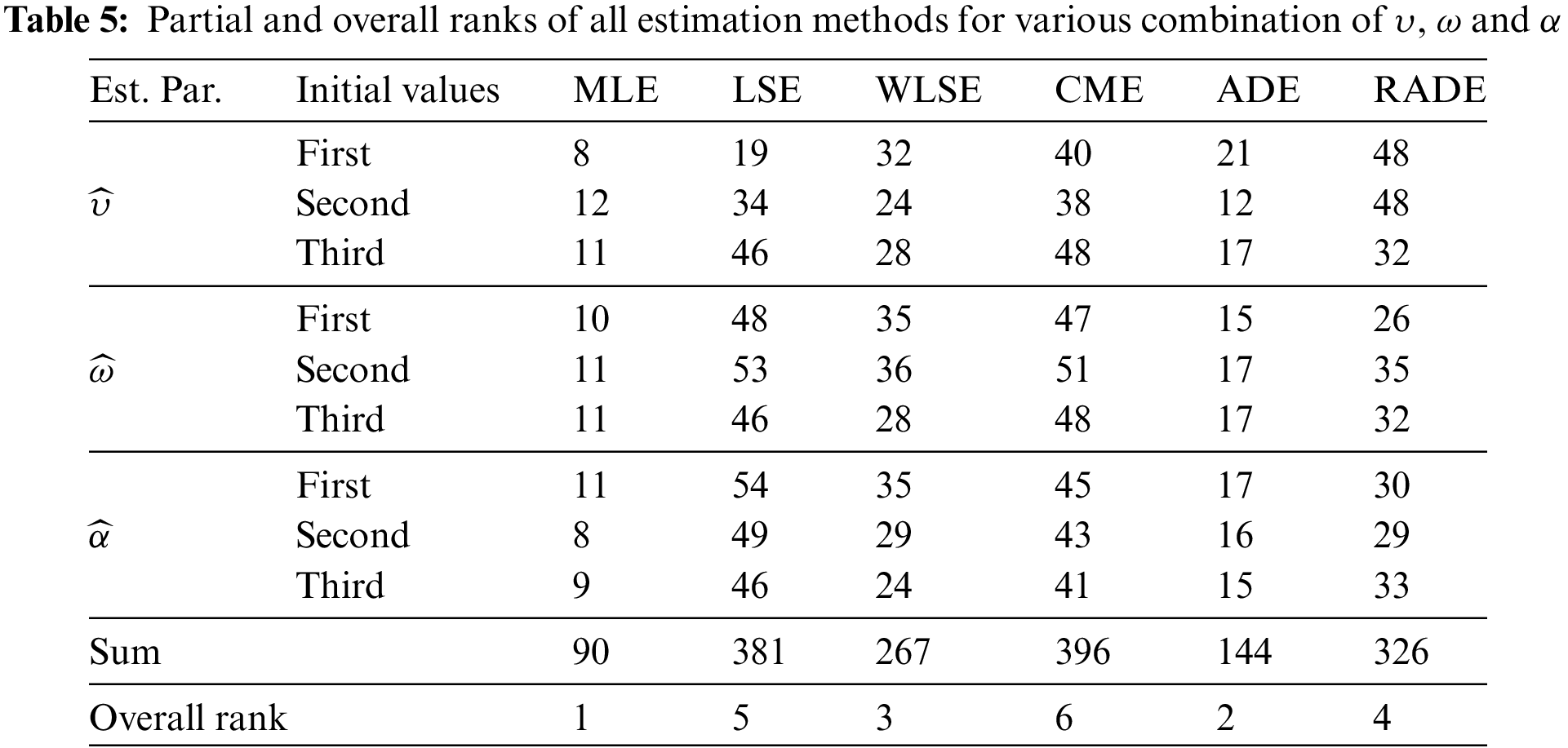
The AB and RMSE of the MLE, CME, LSE, ADE, WLSE, and RADE are presented in Tables 2–4. Moreover, the partial and overall ranks of the estimators are calculated in Table 5. From the values in these tables, one can note that

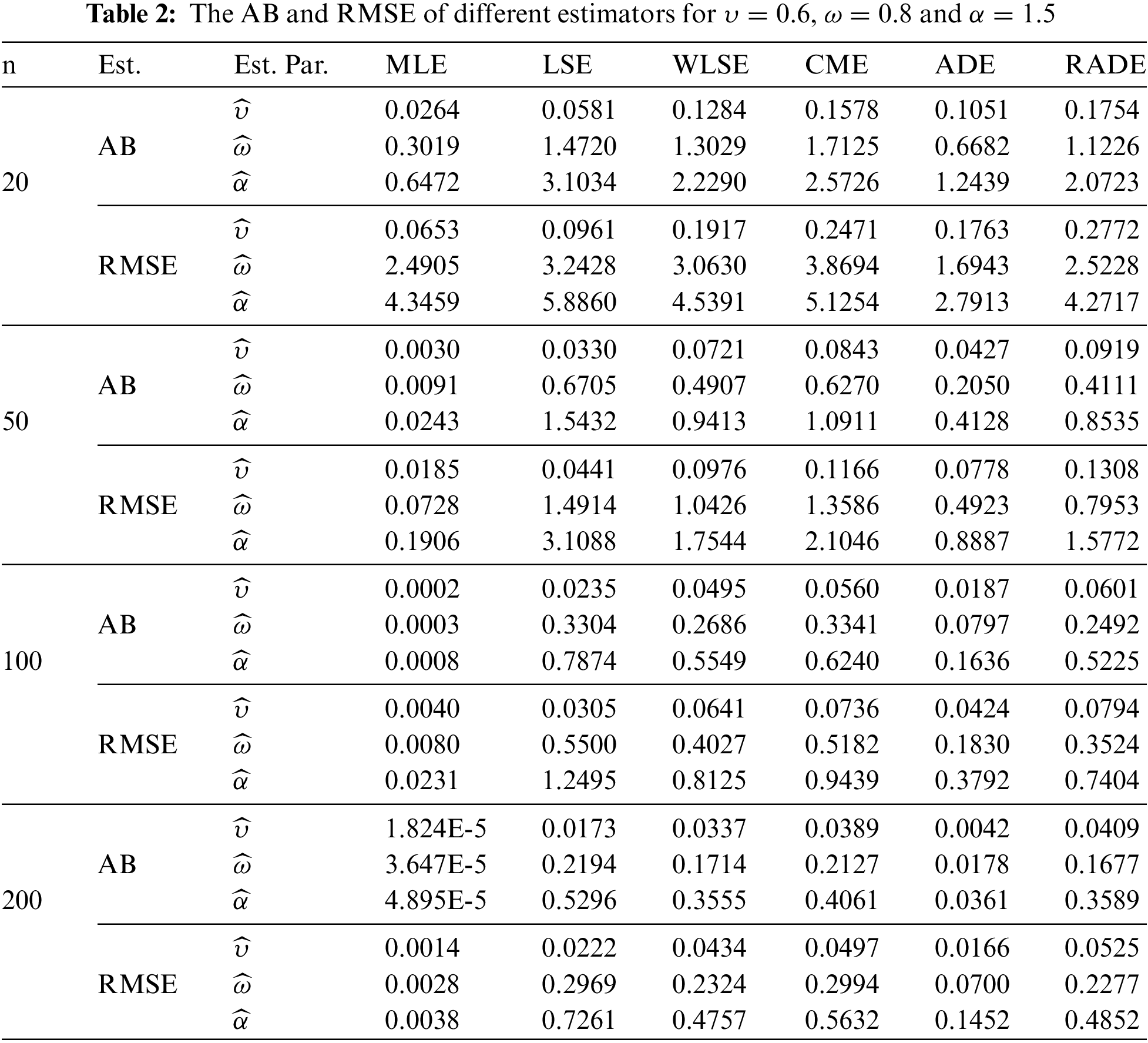
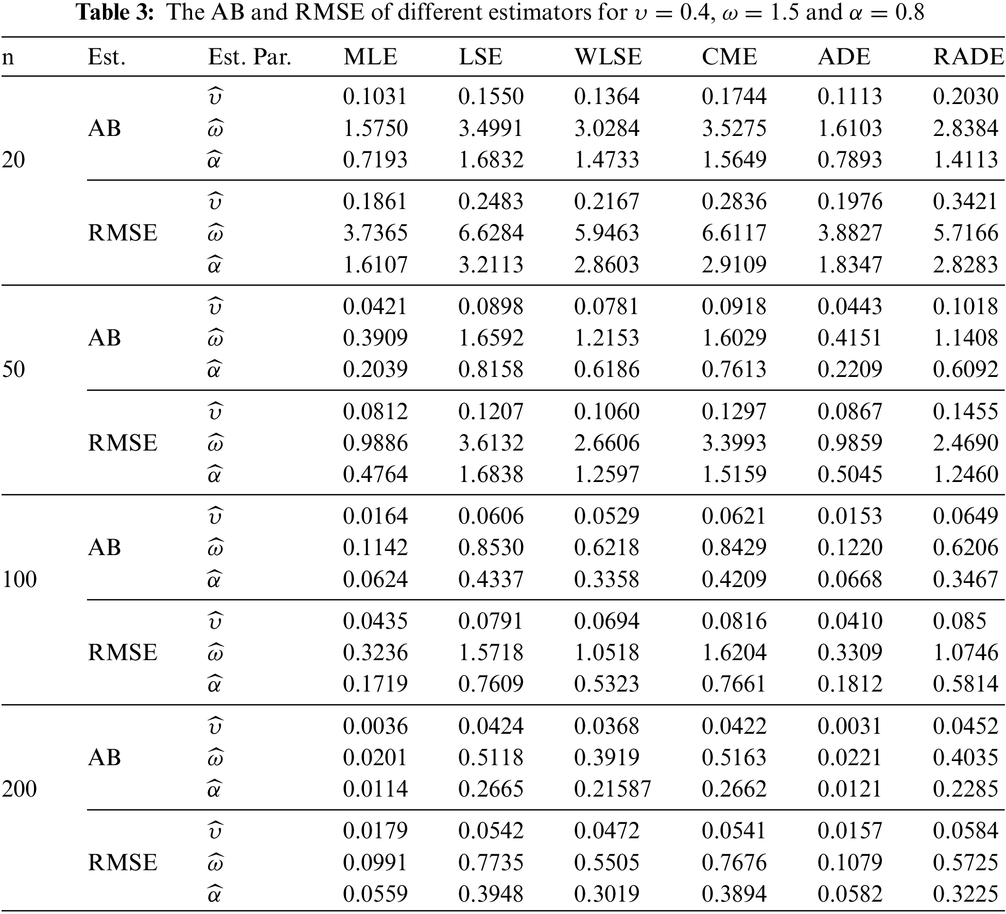
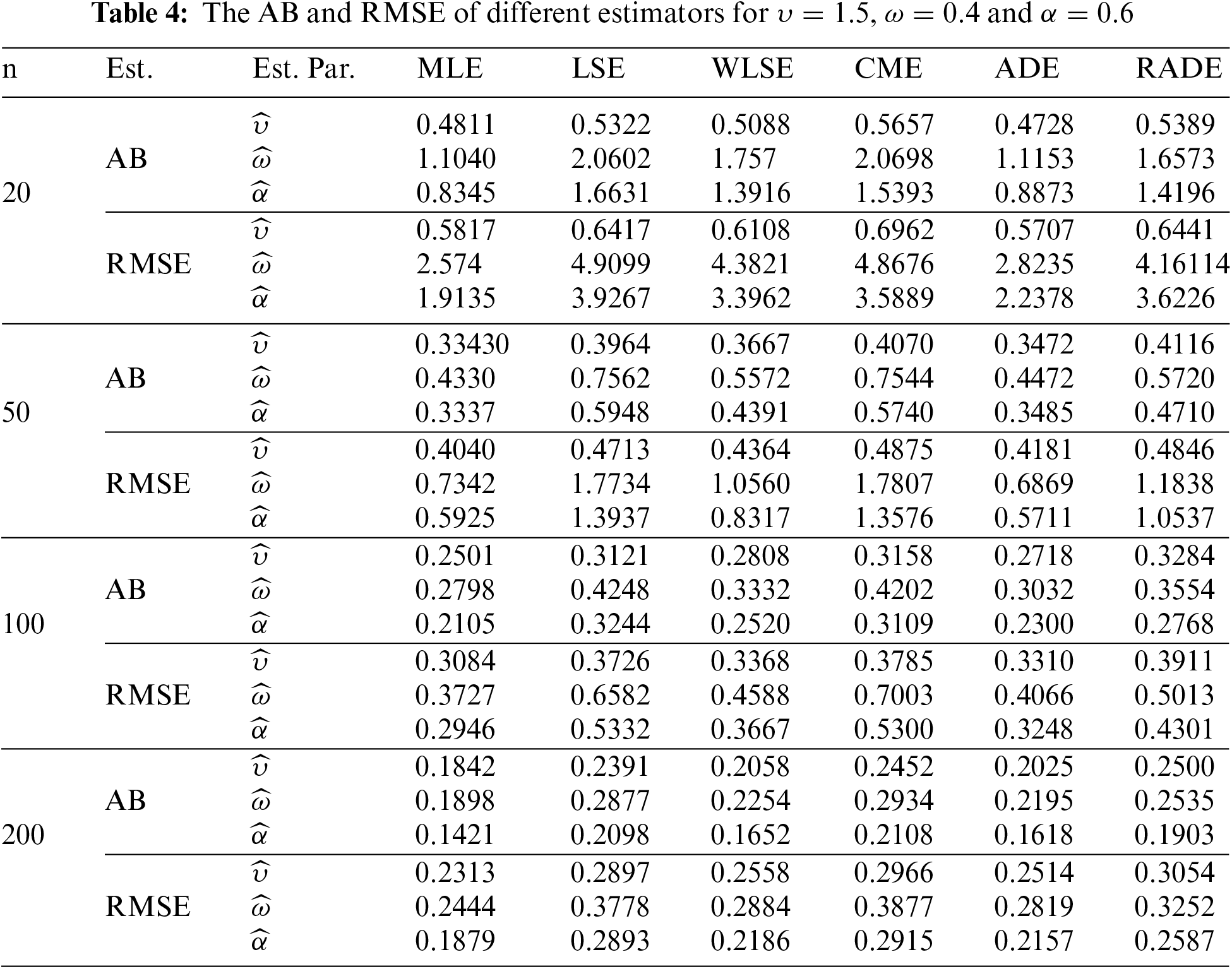
1.   All estimates show the property of consistency, i.e., the AB and RMSE decrease as sample size increases for all parametric combinations.

2.   According to AB and RMSE, the ordering of performance of estimators (from best to worst) for all parameters is the MLE, ADE, WLSE, RADE, LSE and CME.

7  Real-Life Applications

In this section, we analyze two real-life data sets to demonstrate the performance of the LL distribution in practice. Two real-life data sets are fitted to compare the proposed LL model with other five known competitors, namely:

1.   The Exponentiated Lomax (EL) distribution [23] with pdf

g(x;β,λ,α)=λβα(1+xα)−λ−1(1−(1+xα)−λ)β−1,x>0,β,λ,α>0.

2.   The Poisson–Lomax (PoL) distribution [24] with pdf

g(x;β,λ,α)=λαβ1−exp⁡(−λ)(1+βx)−α−1exp⁡[−λ(1+βx)−α],x>0,β,λ,α>0.

3.   The Lomax-Rayleigh (LR) distribution [25] with pdf

g(x;λ,α)=2λαx(1+x2α)−λ−1,x>0,β,λ,α>0.

4.   The power Lomax (PL) distribution [26] with pdf

g(x;β,λ,α)=λβαxβ−1(1+xβα)−λ−1,x>0,β,λ,α>0.

5.   The Lomax (L) distribution [27] with pdf

g(x;λ,α)=λα(1+xα)−λ−1,x>0,λ,α>0.

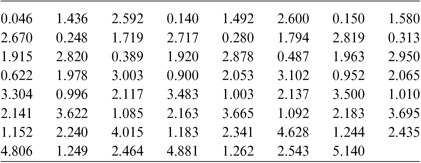
The first data represent 63 service times (thousand hours) of aircraft windshield (unit in thousand hours) as reported in Murthy et al. [28]. The data are as follows:

The second data represents 63 strengths of 1.5 cm glass fibers which are measured by the National Physical Laboratory, in England as reported in Smith et al. [29]. The data are as follows:

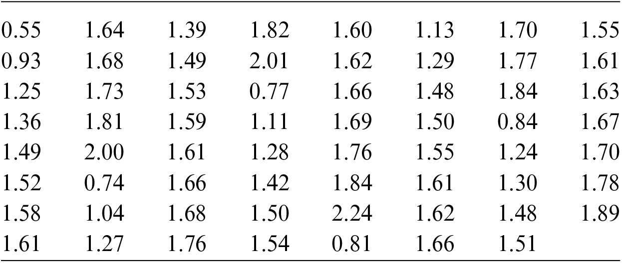
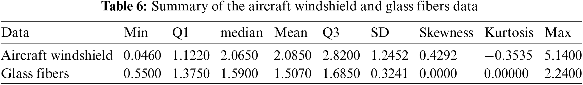
Table 6 provides a brief summary for both data sets.

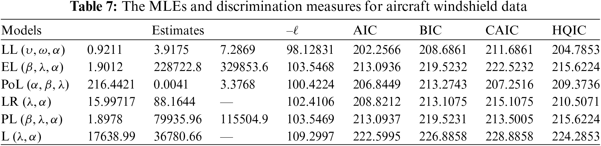
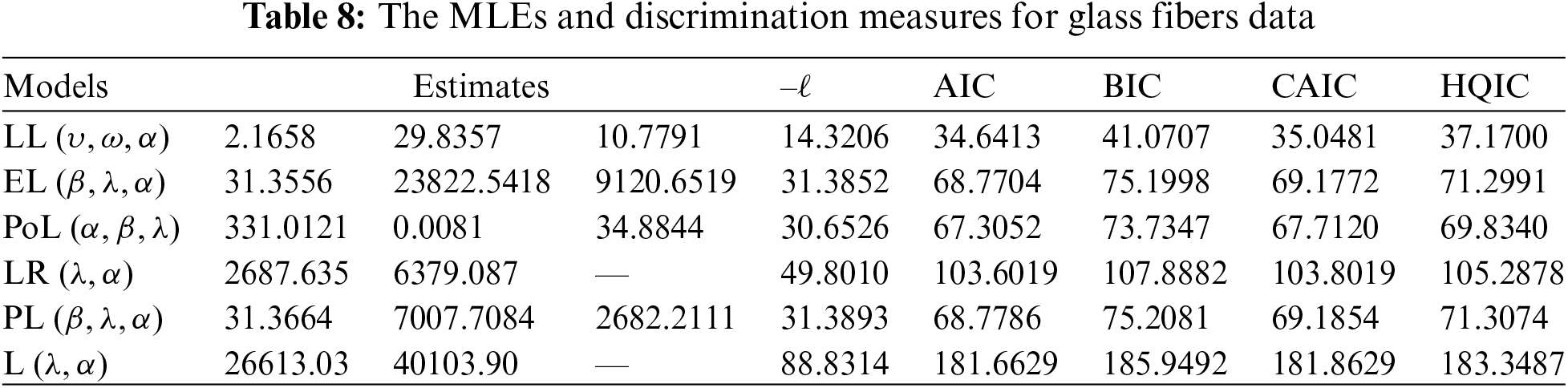
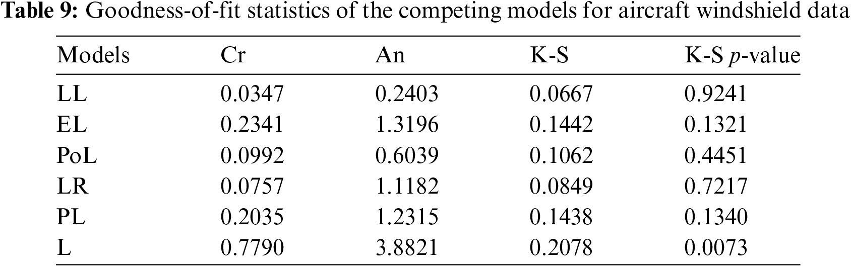
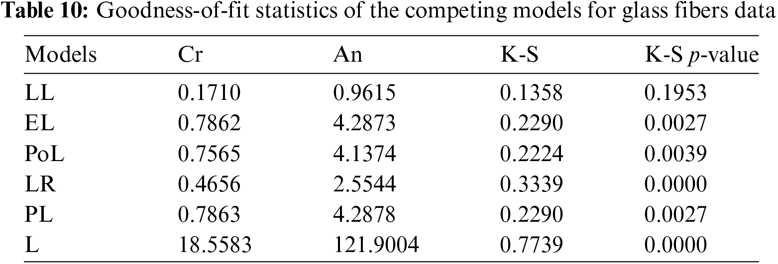
The parameters of the fitted distributions are estimated using the ML method and some discrimination measures are calculated to explore the efficiency of the competing distributions. These measures include the Akaike information criterion (AIC), Bayesian IC (BIC), corrected AIC (CAIC), Hannan–Quinn IC (HQIC), and –ℓ, where ℓ is the maximized log-likelihood. Additionally, goodness-of-fit statistics such as Anderson–Darling (An), Cramér–von Mises (Cr), and Kolmogorov–Smirnov (K-S) with its corresponding p-value (K-S p-value) are also calculated. More details about the goodness-of-fit statistics can be explored by Shama et al. [30].

Tables 7 and 8 present the MLEs of the parameters of the fitted distributions along with their discrimination measures for both data sets, respectively. Based on Tables 7 and 8, we conclude that the LL distribution is the best model as compared to other Lomax extensions. Tables 9 and 10 provide the values of goodness-of-fit measures of the LL model and other models for the two data sets. These results also indicate that the LL model provides a better fit to aircraft windshield and glass fibers data as compared to other Lomax models.

The probability-probability (P-P) plots of the fitted distributions for both data sets are provided in Figs. 4 and 5. The fitted density, cdf, sf, and P-P plots of the LL distribution for both data sets are displayed in Figs. 6 and 7. The plots support the results in Tables 7–10 and illustrate that the LL distribution provides a better approximation between the theoretical and empirical curves. Furthermore, Figs. 8 and 9 present the histograms of aircraft windshield and glass fibers data along with the fitted densities of the LL model and other studied distributions. All plots provide evidence that the LL distribution is the most well-adjusted model for aircraft windshield and glass fibers data.

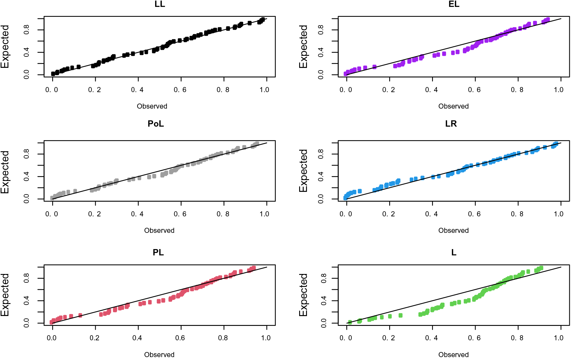
Figure 4: P-P plots for aircraft windshield data

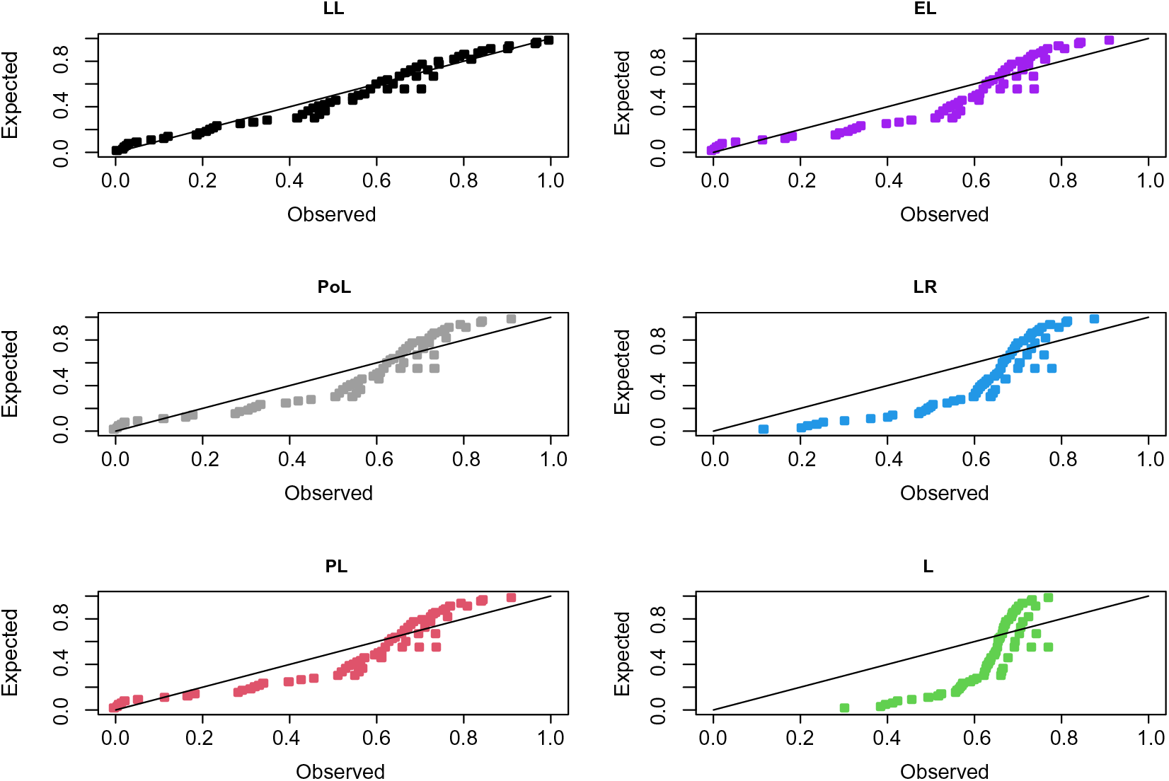
Figure 5: P-P plots for glass fibers data

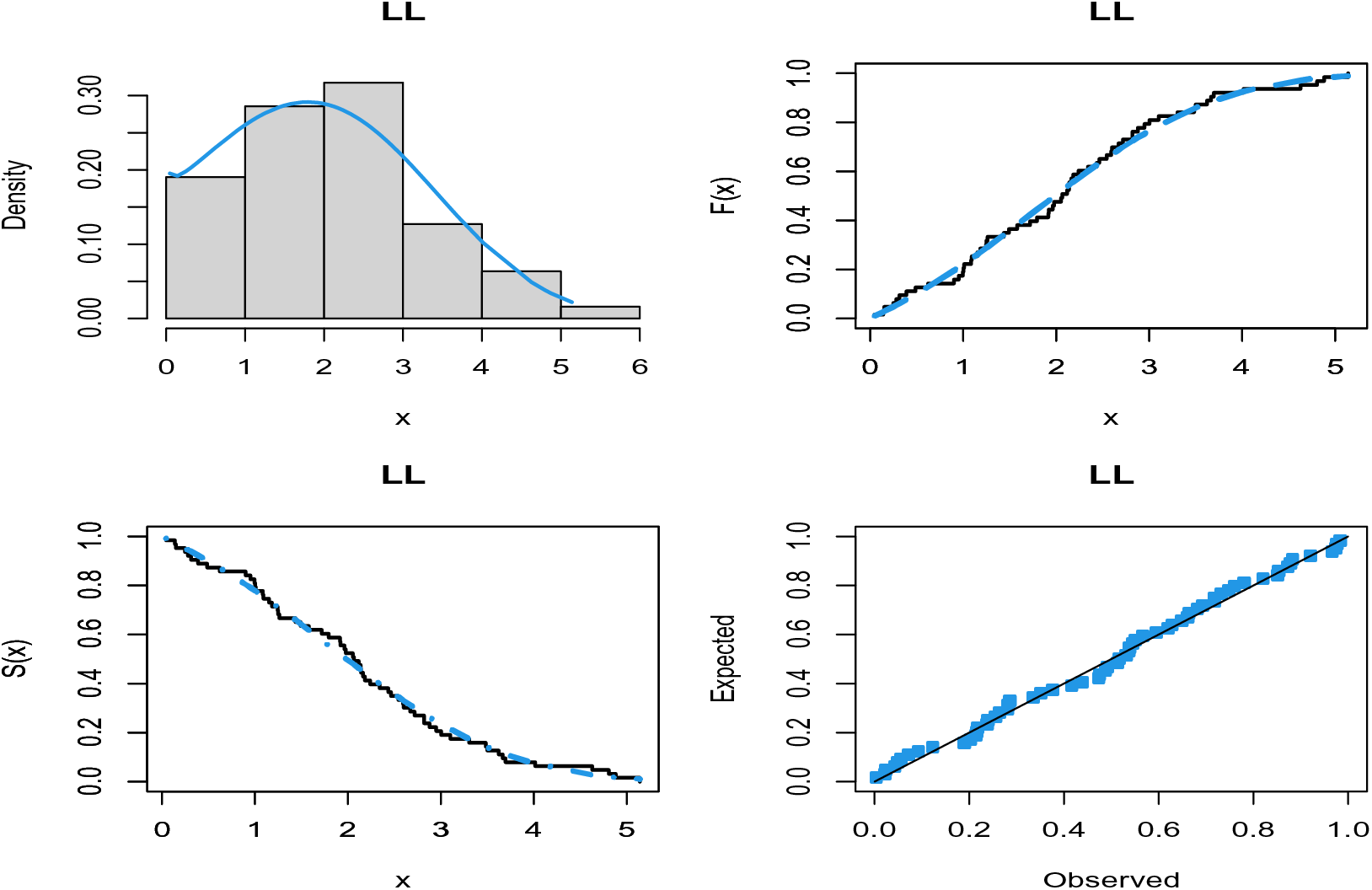
Figure 6: Plots of the fitted functions of the LL model for aircraft windshield data

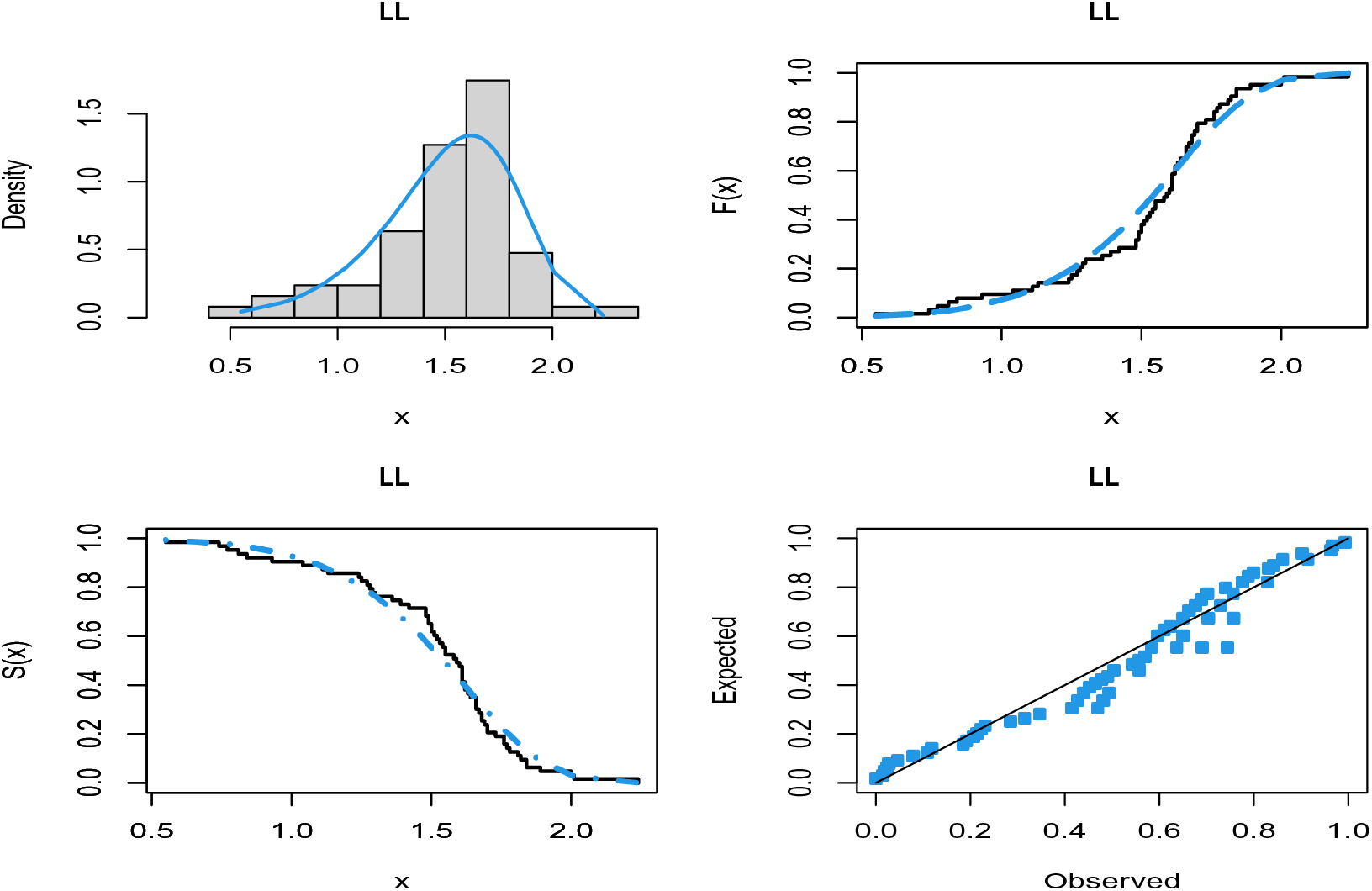
Figure 7: Plots of the fitted functions of the LL model for glass fibers data

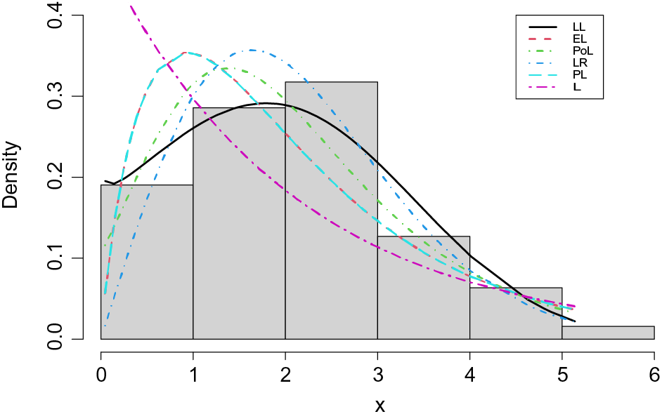
Figure 8: Histogram of aircraft windshield data along with the estimated densities

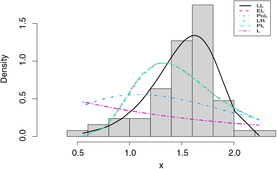
Figure 9: Histogram of glass fibers data along with the estimated densities

8  Conclusions

This study introduces a new flexible family called the LG family. Its special sub-models can represent various shapes of aging failure criteria, including monotonic and non-monotonic failure rates. The densities of the sub-models of the LG family can be reversed-J shaped, right-skewed, symmetric, left-skewed, decreasing-increasing-decreasing densities. One of its special models, namely the LL, is studied in detail. The failure rate shapes of the LL distribution are derived and proved mathematically. In addition, various statistical properties of the LL distribution are investigated. Six estimation methods are employed to estimate the LL parameters, and their performance is explored via simulation results. The numerical experiments illustrate the accuracy of the maximum likelihood; hence, they are recommended for estimating the LL parameters. Two real-life datasets are analyzed, indicating that the LL distribution can provide a better fit for modeling actual data compared to some competing Lomax models.

The perspectives of this study can include the development of a bivariate LL distribution and the construction of a discrete version of the LL model.

Acknowledgement: The authors would like to thank the editor and the referees for valuable comments which greatly improved the paper.

Funding Statement: The authors received no specific funding for this study.

Author Contributions: The authors confirm contribution to the paper as follows: study conception and design: J.N.A.A., A.Z.A., B.A., M.S.S.; data collection: A.Z.A., M.S.S.; analysis and interpretation of results: J.N.A.A., A.Z.A., B.A., M.S.S.; draft manuscript preparation: J.N.A.A. All authors reviewed the results and approved the final version of the manuscript.

Availability of Data and Materials: This work is mainly a methodological development and has been applied on secondary data which are provided in the manuscript.

Conflicts of Interest: The authors declare that they have no conflicts of interest to report regarding the present study.

References

1. Cordeiro, G. M., de Castro, M. (2011). A new family of generalized distributions. Journal of Statistical Computation and Simulation, 81, 883–893. [Google Scholar]

2. Alzaghal, A., Lee, C., Famoye, F. (2013). Exponentiated T-X family of distributions with some applications. International Journal of Probability and Statistics, 2, 31–49. [Google Scholar]

3. Bourguignon, M., Silva, R. B., Cordeiro, G. M. (2014). The Weibull-G family of probability distributions. Journal of Data Science, 12, 53–68. [Google Scholar]

4. Haq, M. A. U., Handique, L., Chakraborty, S. (2018). The odd moment exponential family of distributions: Its properties and applications. International Journal of Applied Mathematics and Statistics, 57, 47–62. [Google Scholar]

5. Cordeiro, G. M., Yousof, H. M., Ramires, T. G., Ortega, E. M. (2018). The Burr XII system of densities: Properties, regression model and applications. Journal of Statistical Computation and Simulation, 88, 432–456. [Google Scholar]

6. Haq, M. A. U., Elgarhy, M., Hashmi, S. (2019). The generalized odd Burr III family of distributions: Properties, applications and characterizations. Journal of Taibah University for Science, 13, 961–971. [Google Scholar]

7. Altun, E., Alizadeh, M., Afify, A. Z., Ozel, G. (2019). The generalized odd half-logistic family of distributions with regression models. International Journal of Statistics & Economics, 20, 88–110. [Google Scholar]

8. Nassar, M., Kumar, D., Dey, S., Cordeiro, G. M., Afify, A. Z. (2019). The Marshall-Olkin alpha power family of distributions with applications. Journal of Computational and Applied Mathematics, 351, 41–53. [Google Scholar]

9. Ahmad, Z., Mahmoudi, E., Roozegar, R., Alizadeh, M., Afify, A. Z. (2021). A new exponential-X family: Modeling extreme value data in the finance sector. Mathematical Problems in Engineering, 2021, 1–14. [Google Scholar]

10. Aljohani, H. M., Bandar, S. A., Al-Mofleh, H., Ahmad, Z., El-Morshedy, M. et al. (2022). A new asymmetric extended family: Properties and estimation methods with actuarial applications. PLoS One, 17, e0275001. [Google Scholar] [PubMed]

11. Shama, M. S., El Ktaibi, F., Al Abbasi, J. N., Chesneau, C., Afify, A. Z. (2023). Complete study of an original power-exponential transformation approach for generalizing probability distributions. Axioms, 12, 67. [Google Scholar]

12. Corless, R. M., Gonnet, G. H., Hare, D. E. G., Jeffrey, D. J., Knuth, D. E. (1996). On the Lambert W function. Advances in Computational Mathematics, 5, 329–359. [Google Scholar]

13. Visser, M. (2018). Primes and the Lambert W function. Mathematics, 6, 56. [Google Scholar]

14. Goerg, G. M. (2011). Lambert W random variables—A new family of generalized skewed distributions with applications to risk estimation. Annals of Applied Statistics, 5, 2197–2230. [Google Scholar]

15. Iriarte, Y. A., de Castro, M., Gómez, H. W. (2020). The Lambert-F distributions class: An alternative family for positive data analysis. Mathematics, 8, 1398. [Google Scholar]

16. Lai, C., Xie, M., Murthy, D. (2003). A modified Weibull distribution. IEEE Transactions on Reliability, 52, 7–33. [Google Scholar]

17. Swain, J., Venkatraman, S., Wilson, J. R. (1988). Least squares estimation of distribution function in Johnsons translation system. Journal of Statistical Computation and Simulation, 29, 271–297. [Google Scholar]

18. Choi, K., Bulgren, W. (1968). An estimation procedure for mixtures of distributions. Journal of the Royal Statistical Society Series B:Methodological, 30, 444–460. [Google Scholar]

19. Boos, D. D. (1981). Minimum distance estimators for location and goodness of fit. Journal of the American Statistical Association, 76, 663–670. [Google Scholar]

20. Anderson, T. W., Darling, D. A. (1952). Asymptotic theory of certain “goodness of fit” criteria based on stochastic processes. The Annals of Mathematical Statistics, 23, 193–212. [Google Scholar]

21. Anderson, T. W., Darling, D. A. (1954). A test of goodness of fit. Journal of the American Statistical Association, 49, 765–769. [Google Scholar]

22. Luceno, A. (2006). Fitting the generalized Pareto distribution to data using maximum goodness-of-fit estimators. Computational Statistics & Data Analysis, 51, 904–917. [Google Scholar]

23. Gupta, R. C., Gupta, P. I., Gupta, R. D. (1998). Modeling failure time data by Lehmann alternatives. Communications in Statistics-Theory and Methods, 27, 887–904. [Google Scholar]

24. Al-Zahrani, B., Sagor, H. (2014). The Poisson-Lomax distribution. Revista Colombiana de Estadística, 37, 225–245. [Google Scholar]

25. Venegas, O., Iriarte, Y. A., Astorga, J. M., Borger, A., Bolfarine, H. et al. (2019). Lomax-Rayleigh distribution with an application. Applied Mathematics & Information Sciences, 13, 741–748. [Google Scholar]

26. Rady, E. A., Hassanein, W. A., Elhaddad, T. A. (2016). The power Lomax distribution with an application to bladder cancer data. Springerplus, 5, 1838. [Google Scholar] [PubMed]

27. Lomax, K. S. (1954). Business failures: Another example of the analysis of failure data. Journal of the American Statistical Association, 49, 847–852. [Google Scholar]

28. Murthy, D. N. P., Xie, M., Jiang, R. (2004). Weibull models, wiley series in probability and statistics. New York: John Wiley and Sons. [Google Scholar]

29. Smith, R., Naylor, J. (1987). A comparison of maximum likelihood and Bayesian estimators for the three-parameter Weibull distribution. Applied Statistics, 36, 358–369. [Google Scholar]

30. Shama, M. S., Dey, S., Altun, E., Afify, A. Z. (2022). The gamma-Gompertz distribution: Theory and applications. Mathematics and Computers in Simulation, 193, 689–712. [Google Scholar]