
 Submit a Paper
 Propose a Special lssue
 Open Access
ARTICLE

Uniaxial Compressive Strength Prediction for Rock Material in Deep Mine Using Boosting-Based Machine Learning Methods and Optimization Algorithms
School of Resources and Safety Engineering, Central South University, Changsha, 410083, China
* Corresponding Author: Diyuan Li. Email:
Computer Modeling in Engineering & Sciences 2024, 140(1), 275-304. https://doi.org/10.32604/cmes.2024.046960
Received 20 October 2023; Accepted 24 January 2024; Issue published 16 April 2024
 View Full Text
 Download PDF
Abstract
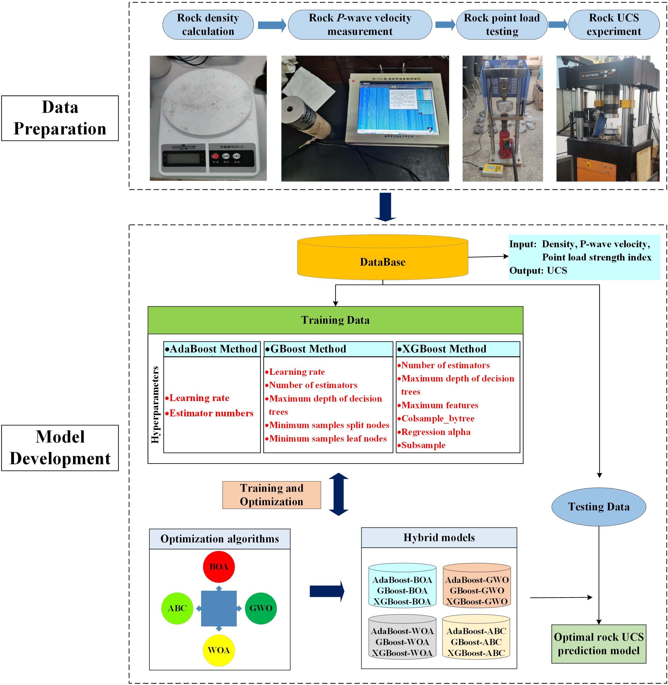
Traditional laboratory tests for measuring rock uniaxial compressive strength (UCS) are tedious and time-consuming. There is a pressing need for more effective methods to determine rock UCS, especially in deep mining environments under high in-situ stress. Thus, this study aims to develop an advanced model for predicting the UCS of rock material in deep mining environments by combining three boosting-based machine learning methods with four optimization algorithms. For this purpose, the Lead-Zinc mine in Southwest China is considered as the case study. Rock density, P-wave velocity, and point load strength index are used as input variables, and UCS is regarded as the output. Subsequently, twelve hybrid predictive models are obtained. Root mean square error (RMSE), mean absolute error (MAE), coefficient of determination (R2), and the proportion of the mean absolute percentage error less than 20% (A-20) are selected as the evaluation metrics. Experimental results showed that the hybrid model consisting of the extreme gradient boosting method and the artificial bee colony algorithm (XGBoost-ABC) achieved satisfactory results on the training dataset and exhibited the best generalization performance on the testing dataset. The values of R2, A-20, RMSE, and MAE on the training dataset are 0.98, 1.0, 3.11 MPa, and 2.23 MPa, respectively. The highest values of R2 and A-20 (0.93 and 0.96), and the smallest RMSE and MAE values of 4.78 MPa and 3.76 MPa, are observed on the testing dataset. The proposed hybrid model can be considered a reliable and effective method for predicting rock UCS in deep mines.Graphic Abstract
Keywords
Nomenclature
| Density | |
| P-wave velocity | |
| Point load strength | |
| UCS | Uniaxial compressive strength |
As one of the most critical parameters of rock strength, uniaxial compressive strength (UCS) is widely used in geotechnical engineering, tunneling, and mining engineering. The reliability of acquiring rock UCS in situ directly influences subsequent operations, such as drilling, digging, blasting, and support. Typically, the UCS value of rock materials can be obtained by following the well-established regulations of the International Society for Rock Mechanics (ISRM) [1] and the American Society for Testing Materials (ASTM) [2]. Laboratory testing has strict requirements for specimen preparation. It is challenging to obtain high-quality rock samples from layered sedimentary rocks, highly weathered rocks, and fractured rock masses [3–6]. Moreover, the accuracy of laboratory testing depends on the professionalism of the operators. For this reason, other highly efficient and straightforward methods for rock UCS prediction have been developed in various studies, such as statistical methods (single regression analysis methods and multiple variable regression methods) and soft computing-based methods.
Several studies have employed statistical equations to investigate the relationship between a single variable and UCS [7,8]. Fener et al. [9] conducted several laboratory tests and developed an equation for rock UCS prediction based on point load test results, achieving better performance with an R2 value of 0.85. Yasar et al. [10] investigated the relationships between hardness (Shore Scleroscope hardness and Schmidt hammer hardness) and UCS, revealing that the hardness property showed a high correlation coefficient with rock UCS. Yilmaz [11] introduced a new testing method to determine the UCS of rock, called the core strangle test (CST). The UCS prediction results obtained from CST were more accurate than those from the point load tests. Basu et al. [12] pointed out that point load strength could be used to predict the UCS of anisotropic rocks, and in their study, the final R2 result reached 0.86. Khandelwal [13] adopted the linear regression method to fit the relationships between P-wave velocity (
However, predicting UCS using a single related factor is not advised because rock strength is determined by a combination of physical and mechanical properties [5]. Multiple regression models have shown better performance in rock UCS prediction than single regression methods. Azimian et al. [5] compared the prediction performance of UCS between the standalone regression model and the multiple regression method. The R2 values of the single regression equations using only
In recent years, artificial intelligence (AI) methods have become widely used in engineering to tackle complex nonlinear problems due to their superior capabilities. They are recommended for solving other complex problems, such as earth pressure calculation and rock profile reconstruction [21,22]. Research reviews have revealed that AI-based methods have been successfully applied in areas such as tunnel squeezing analysis [23,24], rock mass failure mode classification [25], rock lithology classification [26,27], and rock burst prediction and assessment [28–30]. The outstanding results achieved by AI-based methods have garnered significant attention in the prediction of rock mechanical parameters. For example, Ghasemi et al. [31] proposed the M5P model tree method to predict the UCS of carbonate rocks. SHR, n, dry unit weight,
AI-based methods offer distinct advantages over traditional empirical formulas for rock UCS prediction. Traditional approaches to determining UCS through laboratory testing face limitations. These include challenges in obtaining high-quality rock samples from certain geological conditions, such as severely fragmented rock masses, in-situ core disking, and lower efficiency in high-quality rock sample collection. Moreover, few studies have been conducted on predicting the UCS of rock materials in deep mines using boosting-based approaches. Therefore, this study aims to develop a simple and robust rock UCS predictive model tailored for deep mining environments. The Lead-Zinc mine in Southwest China serves as the case study. Three easily accessible parameters
This study considers boosting-based ML methods such as AdaBoost, GBoost, and XGBoost base models for rock UCS prediction. Boosting, an advanced ensemble method, combines several weaker learners to create a strong learner, ensuring improved overall performance of the final model. In addition, four optimization algorithms, namely BOA, ABC, GWO, and WOA, are employed to obtain the optimal parameters for all the base models. These algorithms are renowned for their robustness and efficiency in solving complex optimization problems. They excel in multidimensional and nonlinear search spaces, providing effective solutions in various fields, from engineering to data science. Detailed descriptions of the Boosting-based approaches and the optimization algorithms are provided in the subsequent sections.
2.1 Boosting-Based ML Algorithms
AdaBoost, a typical ensemble boosting algorithm, combines multiple weak learners to form a single strong learner. By adequately considering the weights of all learners, it produces a model that is more accurate and less prone to overfitting. The procedure of the algorithm is outlined below:
(1) Determine the regression error rate of the weak learner.
• Obtain the maximum error;
where
• Estimate the relative error for each sample using the linearity loss function;
• Determine the regression error rate;
where
(2) Determine the weight coefficient
(3) Samples weights updation for the
(4) Build the ultimate learner.
Additionally, the AdaBoost method requires only a few parameter adjustments, such as the decision tree depth, the number of iterations, and the regression loss function. Consequently, it has been extensively used in various fields, including rock mass classification [38], rockburst prediction [39], rock strength estimation [40,41], and tunnel boring machine performance prediction [42].
The GBoost method, another ensemble algorithm, is inspired by gradient descent. It trains a new weak learner based on the negative gradient of the current model loss. This well-trained weak learner is then combined with the existing model. The final model is constructed by repeating these accumulation steps, as shown below:
(1) Initialize the base learner.
where
(2) Calculate the negative gradient. Then, the leaf node region
(3) Obtain the optimal-fitted value
where
(4) Finally, a strong learner could be obtained.
An advantage of GBoost is its flexibility in choosing the loss function, allowing for the use of any continuously differentiable loss function. This characteristic makes the model more resilient to noise. Due to these advantages, GBoost-based methods have achieved considerable success, resulting in many improved versions [43–45].
2.1.3 Extreme Gradient Boosting
XGBoost, an extension of the gradient boosting algorithm, was developed by Chen et al. [46]. This model has robust applications in classification and regression tasks. The primary idea behind the XGBoost approach is to continually produce new trees, with each decision tree being updated based on the difference between the previous tree’s result and the target value, thereby minimizing model bias. Given a dataset
where
where
The XGBoost method combines the loss function and regularization factor into its objective function, resulting in higher generalization than other models, as shown in Eqs. (14), (15). Another distinctive feature of the XGBoost method is its incorporation of a greedy algorithm and an approximation algorithm for searching the split nodes of the tree. The main optimization parameters are the decision tree depth, the number of estimators, and the maximum features. Chang et al. [47] developed an effective model for credit risk assessment using the XGBoost method. Zhang et al. [48] used the XGBoost method to forecast the undrained shear strength of soft clays. In another work, Nguyen-Sy et al. [49] used the XGBoost method to predict the UCS of concrete. The XGBoost model outperforms the artificial neural network (ANN) model, support vector machine (SVM), and other ML methods.
Optimization algorithms are usually designed to automatically find the best global solution within the given search space, shortening the model development cycle and ensuring model robustness. Hence, four well-performing optimization algorithms, i.e., BOA, ABC, GWO, and WOA, were implemented in this study to optimize the parameters of the aforementioned boosting-based ML models for the prediction of rock UCS.
2.2.1 Bayesian Optimization Algorithm
Compared to the commonly used grid search and random search algorithms, the BOA method, proposed by Pelikan et al. [50], fully utilizes prior information to find the parameters that maximize the target function globally. The algorithm comprises two parts: (1) Gaussian process regression, which aims to determine the values of the mean and variance of the function at each point, and (2) constructing the acquisition function, which is employed to obtain the search position of the next iteration, as shown in Fig. 1. BOA has the advantages of fewer iterations and a faster processing speed and has been applied in several fields. Díaz et al. [51] studied the UCS prediction of jet grouting columns based on several ML algorithms and the BOA method. The optimized model obtained significant improvement compared to existing works. Li et al. [26] proposed an intelligent model for rockburst prediction using BOA for hyperparameter optimization. Lahmiri et al. [52] used BOA to obtain the optimal parameters of models for house price prediction. Bo et al. [53] developed an ensemble classifier model to assess tunnel squeezing hazards, with the optimal values of the seventeen parameters obtained utilizing the BOA method. Additionally, Díaz et al. [54] investigated the correlations between activity and clayey soil properties. Thirty-five ML models were introduced in their research to predict the activity using the clayey soil properties, with the BOA method being used to fine-tune the ML models’ hyperparameters, producing promising results.
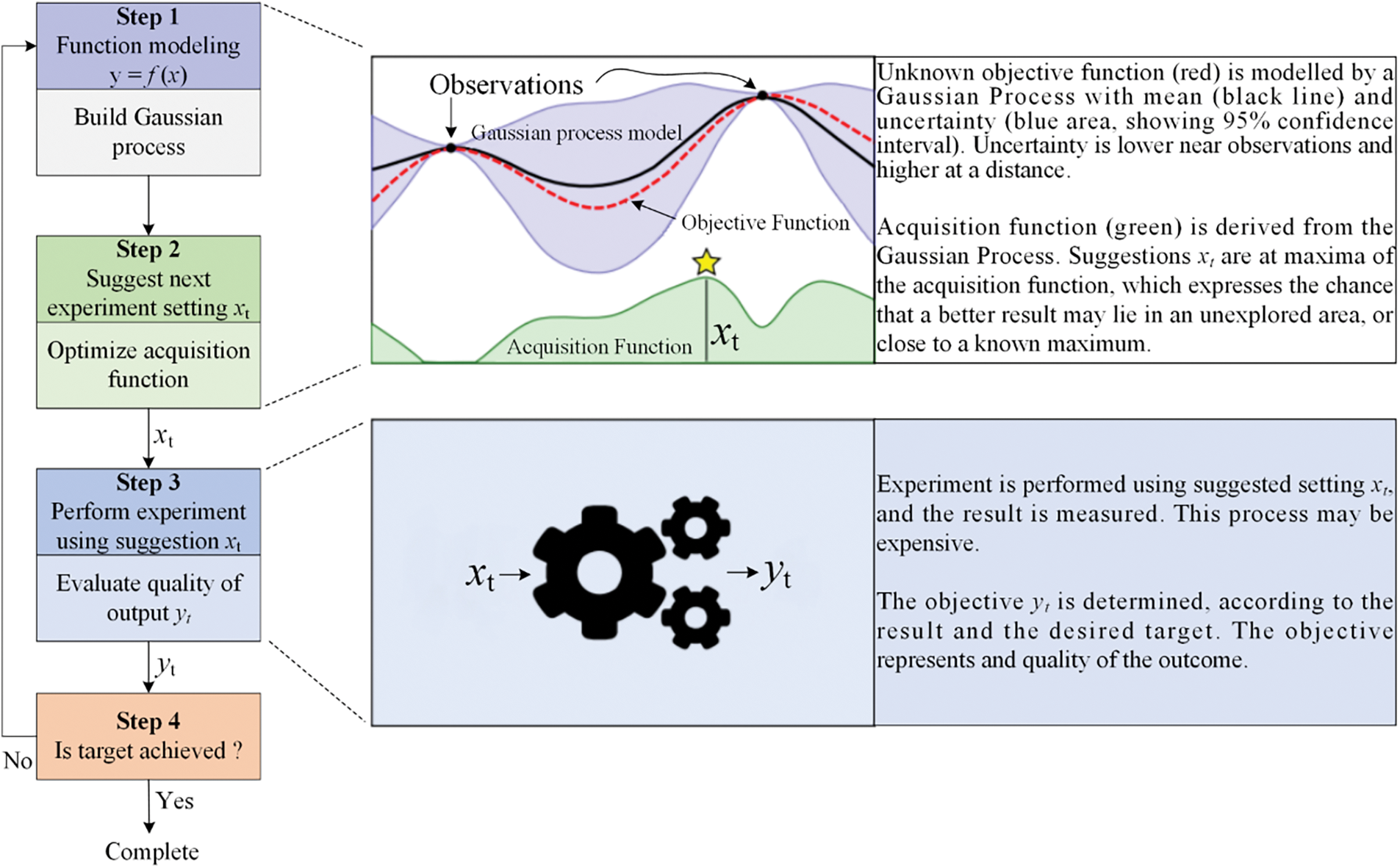
Figure 1: Schematic of the Bayesian optimization algorithm [55]
The ABC method, developed for multivariate function optimization problems by Karaboga [56], divides bees in a colony into three groups (employed, onlookers, and scouts) based on task assignment [57], as illustrated in Fig. 2. Employed bees are tasked with finding available food sources and gathering information. In contrast, onlookers collect good food sources based on data transferred from employed bees and perform further searches for food. Scouts are responsible for finding valuable honey sources around the beehive. In mathematical terms, the food source represents the problem’s solution, and the nectar level equates to the fitness value of the solution [58]. Parsajoo et al. [59] adopted the ABC method to tune and improve the model performance for rock brittleness index prediction. Zhou et al. [60] recommended an intelligent model for rockburst risk assessment and applied the ABC method to obtain optimal hyperparameters for the model. The results revealed ABC to be a valuable and successful strategy.
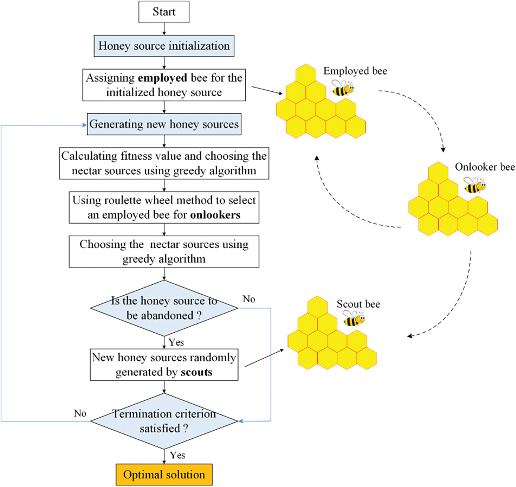
Figure 2: Schematic of the artificial bee colony method
2.2.3 Grey Wolf Optimization Algorithm
GWO is a metaheuristic method developed by Mirjalili et al. [61]. The algorithm simulates grey wolf predation in nature, and wolves are divided into four hierarchies:
where
The constant coefficients
where
During the iteration process, the best solution can be obtained by the head wolves
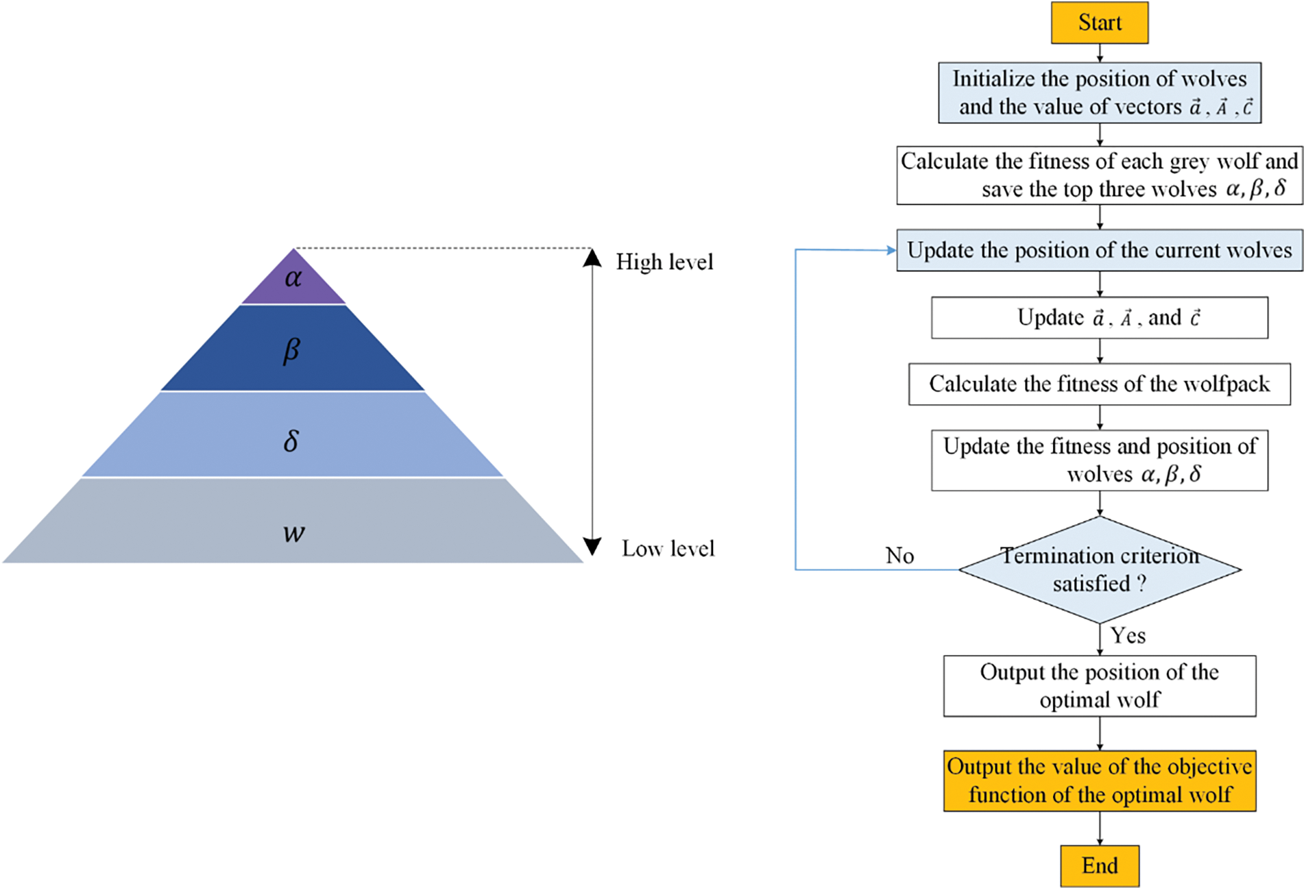
Figure 3: Flowchart of the grey wolf optimization algorithm
2.2.4 Whale Optimization Algorithm
WOA, a unique population intelligence optimization method mimicking whale-feeding behavior, was introduced by Mirjalili et al. [64]. The mathematical modeling process of WOA is comparable to that of the GWO approach. However, a critical distinction between the two algorithms is that humpback whales complete their prey behaviors using either random whale individuals or the ideal individuals, as well as the spiraling bubble-net mode. Zhou et al. [65] applied WOA to obtain optimal parameters for the SVM model for tunnel squeezing classification, achieving higher prediction accuracy. In another study, Tien et al. [66] presented a model for predicting concrete UCS using various optimization techniques, with WOA-based optimization performing the best. Nguyen et al. [67] combined SVM and WOA algorithms to create an intelligent model for predicting fly rock distance, demonstrating that the hybrid WOA-SVM model outperformed standalone models.
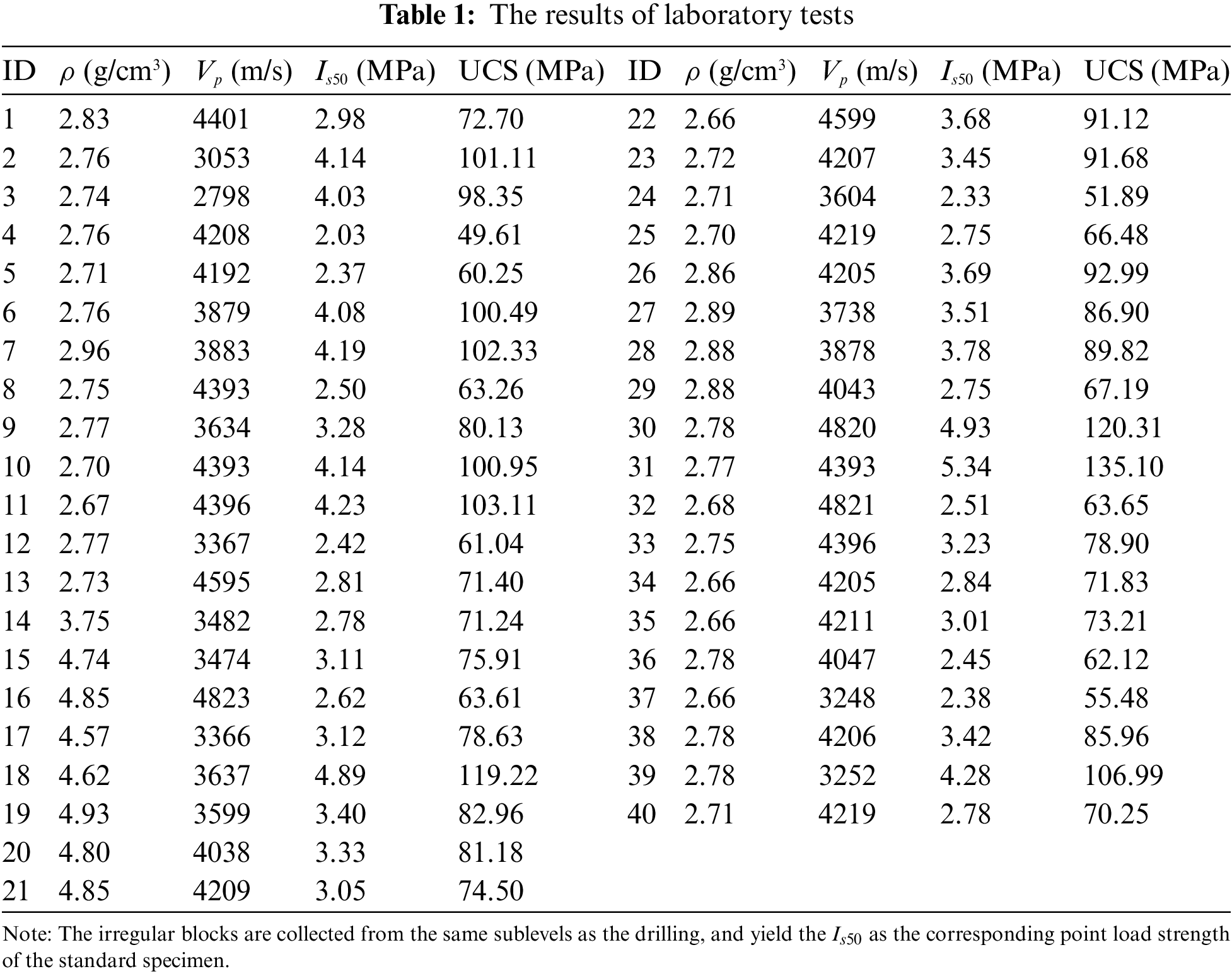
Rock samples collected from a deep lead-zinc ore mine in Yunnan Province, Southwest China, were used as the dataset for developing rock UCS prediction models. The current maximum mining depth of the lead-zinc ore mine has exceeded 1,500 meters, and field rock sample collection operations were conducted at different sublevels, including lower and upper plates surrounding rock and ore, as shown in Fig. 4. All drilling works were done using the KD-100 fully hydraulic pit drilling rig, a small and easy-to-operate machine propelled by compressed air.
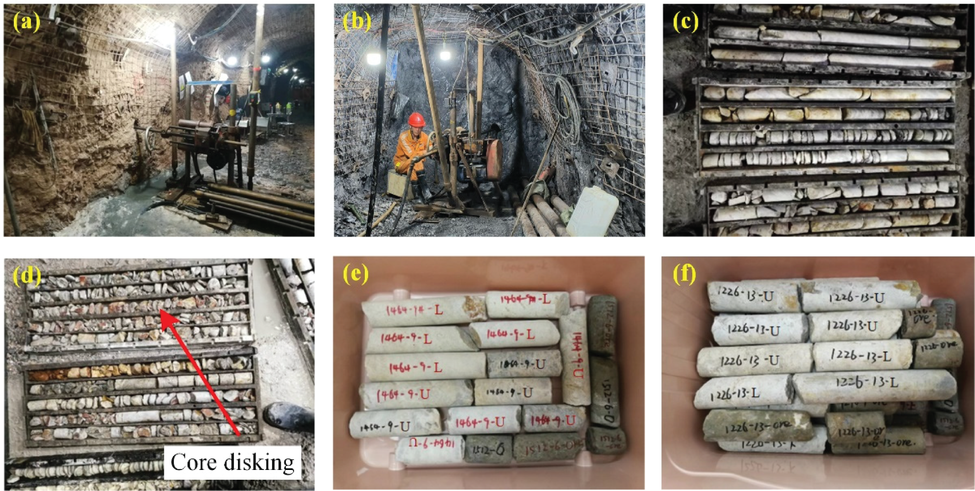
Figure 4: Fieldworks. (a)∼(b) indicate borehole sampling at different sublevels, (c)∼(d) are the collected samples in-situ, (e)∼(f) are the corresponding high-quality samples
After that, all the high-quality samples were made into standard specimens with dimensions of
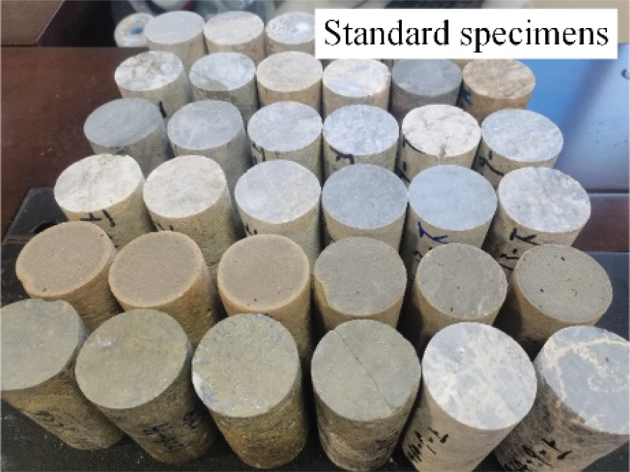
Figure 5: The well-processed standard specimens
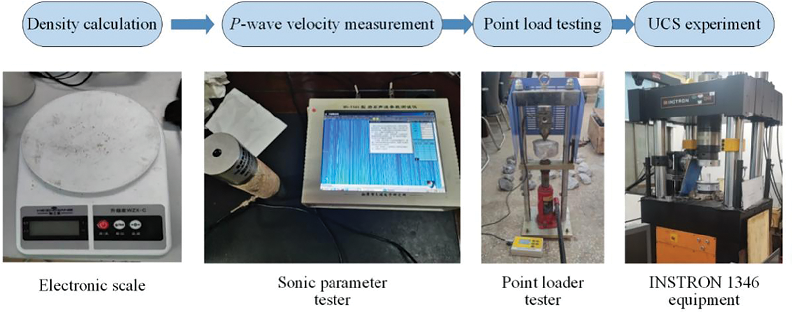
Figure 6: Laboratory tests
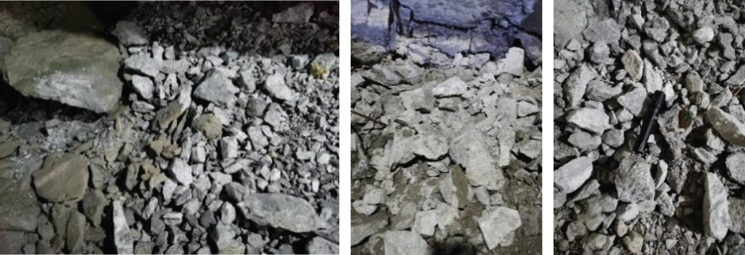
Figure 7: In-situ irregular rock blocks collection for point load testing
For regression prediction problems, correlation analysis between independent and dependent variables is always essential [69]. Fig. 8 shows the analysis results of the correlation between the variables
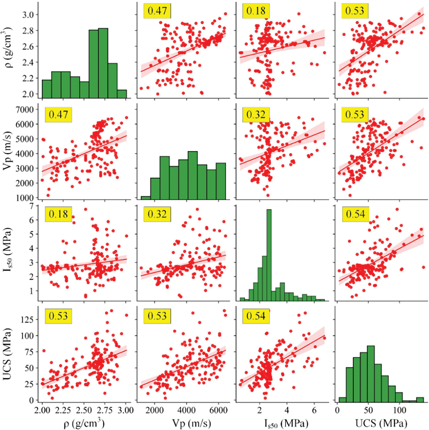
Figure 8: Correlation analysis between input and output variables
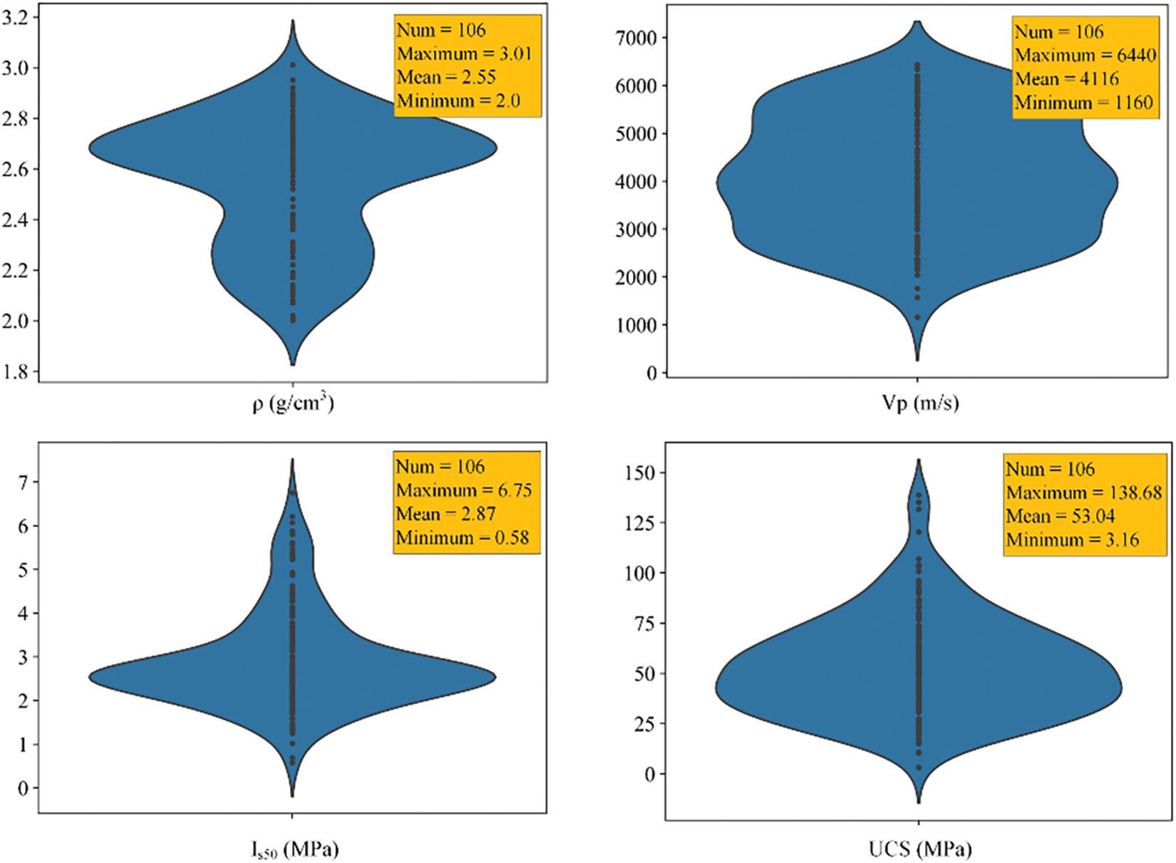
Figure 9: Violin plot of variables
Furthermore, to balance the quantity of training and testing datasets, half of the randomly selected field data and data acquired from the literature were used as training data (86 sets of data), while the remaining field data were used as testing data (20 sets of data). The final ratio between the training and testing data is approximately 8:2.
Simultaneously, all data were normalized prior to model training due to the different magnitudes of the variables. The standardization process was as follows:
where x is the input variables;
The performance of all hybrid models was evaluated using four evaluation indices: root mean square error (RMSE), mean absolute error (MAE), R2, and A-20. Typically, lower values of RMSE and MAE indicate a better model, suggesting that the model’s predictions are closer to the actual values. Conversely, a larger R2 value signifies a more robust model, with a maximum value of 1. The value of A-20 equals the proportion of samples where the mean absolute percentage error between the predicted and actual values is less than 20 percent, as shown in Eq. (25). A larger A-20 value indicates more accurate model predictions.
where
5 Development of the Prediction Models
This study used boosting-based ML algorithms, including AdaBoost, GBoost, and XGBoost, to predict rock UCS. In addition, four optimization approaches, BOA, ABC, GWO, and WOA, were employed to determine the best parameters for all boosting models, ensuring prediction accuracy. The hybrid models were then tested on testing data, providing the optimal rock UCS prediction model. Fig. 10 depicts the flowchart for hybrid model construction.
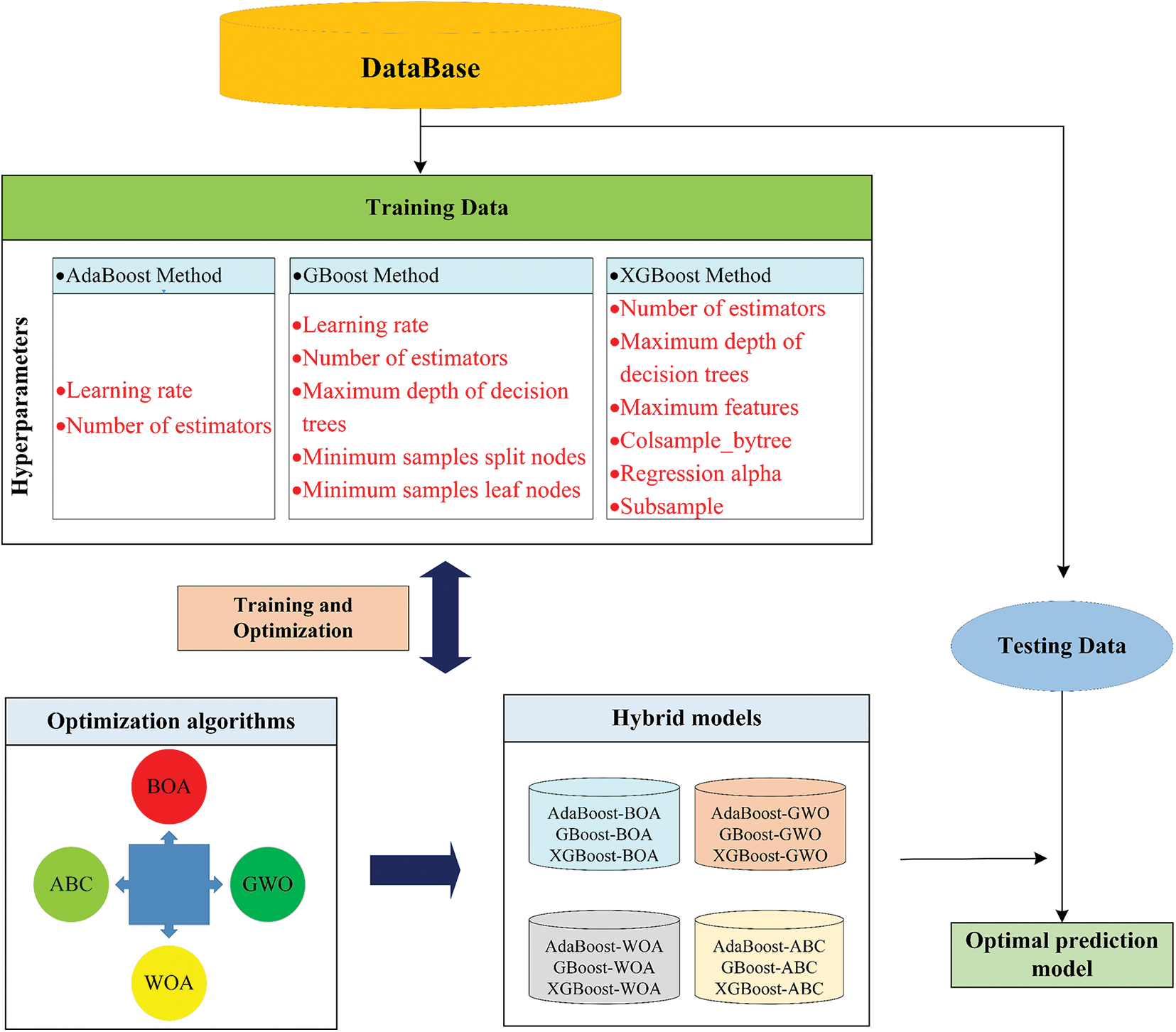
Figure 10: Schematic of the overall framework for rock UCS prediction
5.1 Development of the AdaBoost Model
For the AdaBoost method, the default parameters for regression problems include the base estimator, the number of estimators, the learning rate, and the loss function. The number of estimators and the learning rate were the optimization parameters. However, the base estimator and the loss function were set to their default values (CART decision tree and linear loss function). Additionally, the population size values for the ABC, GWO, and WOA optimization algorithms ranged from 10 to 50, with 5-unit intervals, and the total number of iterations was 100.
To obtain the optimal hyperparameters of the AdaBoost model, the
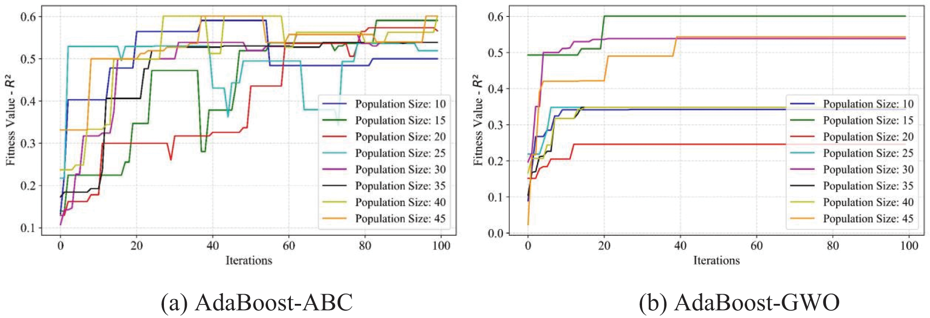
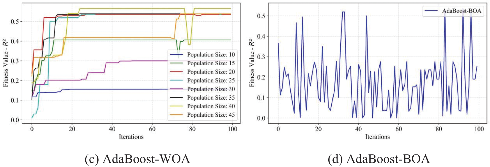
Figure 11: Fitness values of R2 of the AdaBoost model using four optimization methods, ABC, GWO, WOA, and BOA, respectively
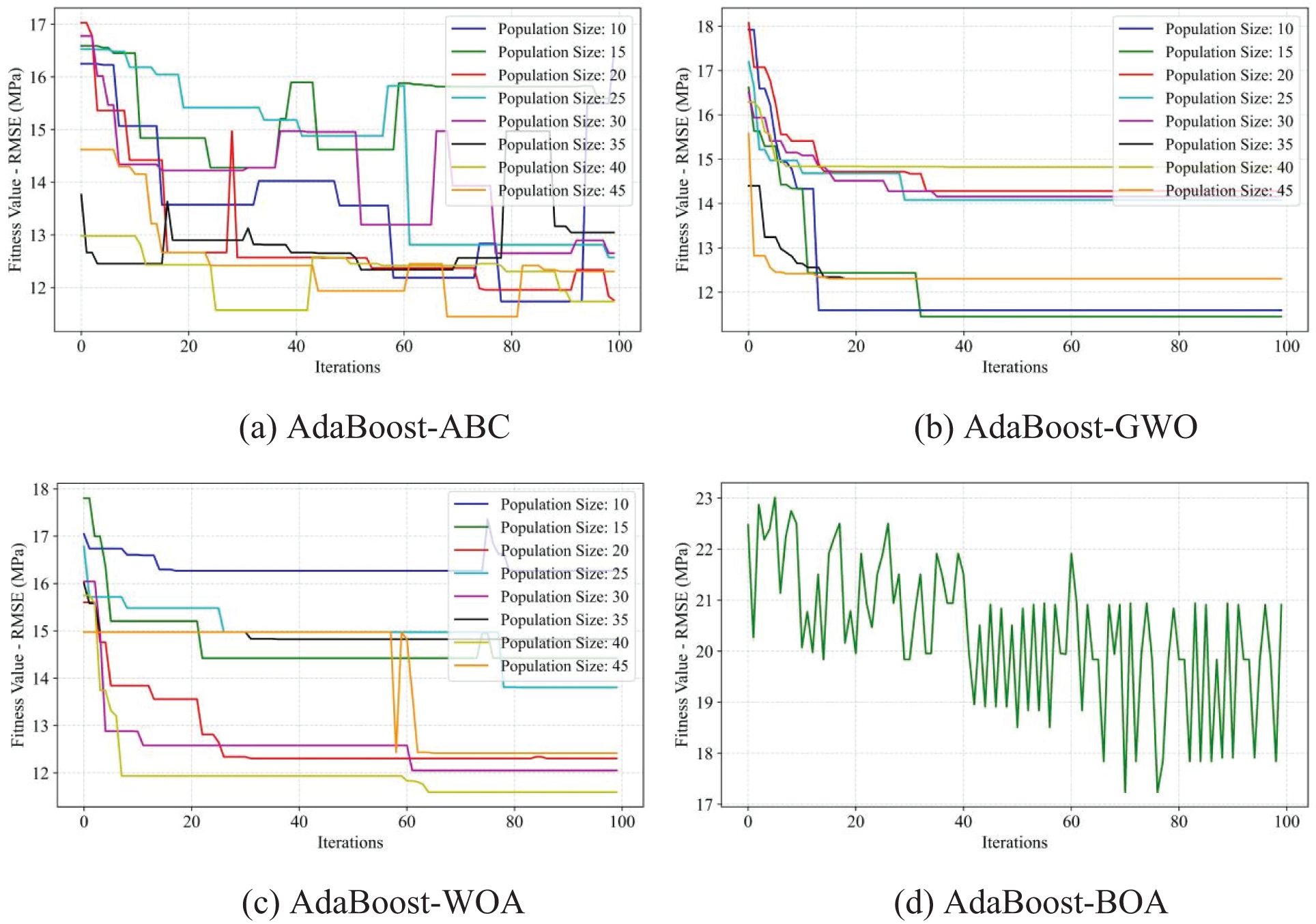
Figure 12: Fitness values of RMSE of the AdaBoost model using four optimization methods, ABC, GWO, WOA, and BOA, respectively
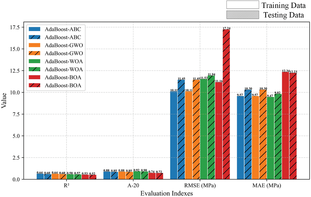
Figure 13: Comparison results of the prediction performance of the AdaBoost hybrid models
5.2 Development of the GBoost Model
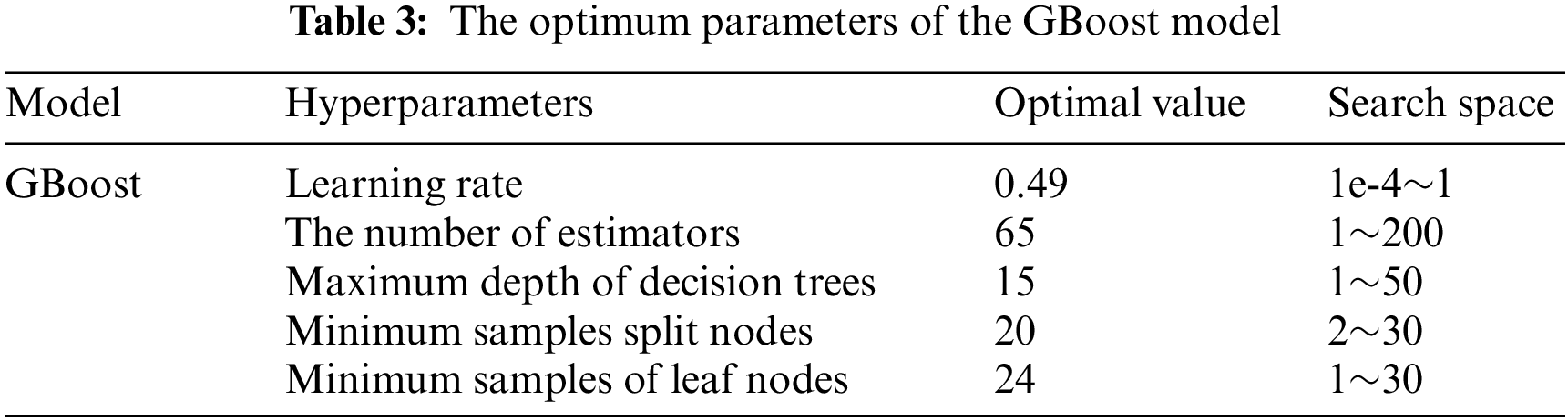
Compared to the AdaBoost model, the GBoost model required fine-tuning of more hyperparameters, including the learning rate, the number of estimators, maximum decision tree depth, minimum sample split node, and minimum sample leaf node. Similarly, the training process and the corresponding results of
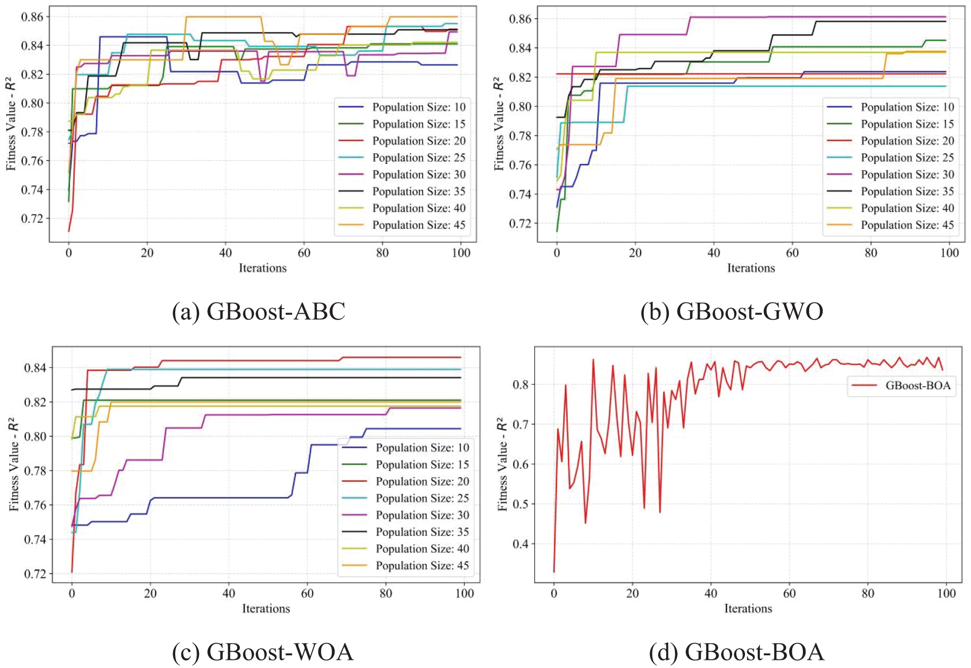
Figure 14: Fitness values of R2 of the GBoost model using four optimization methods, ABC, GWO, WOA, and BOA, respectively
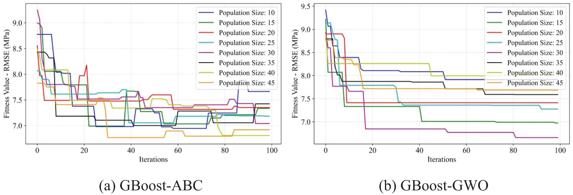
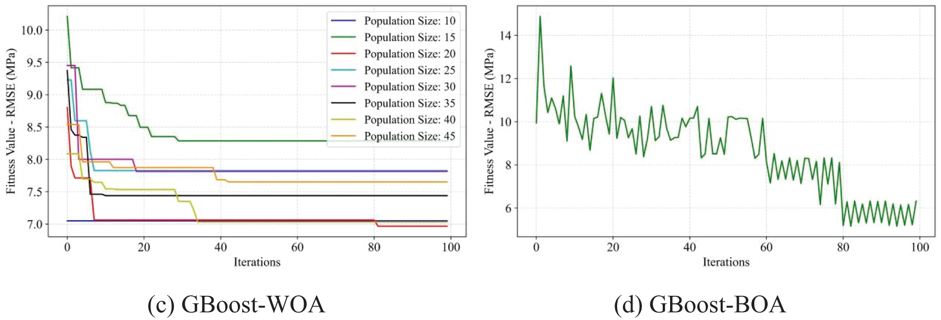
Figure 15: Fitness values of RMSE of the GBoost model using four optimization methods, ABC, GWO, WOA, and BOA, respectively
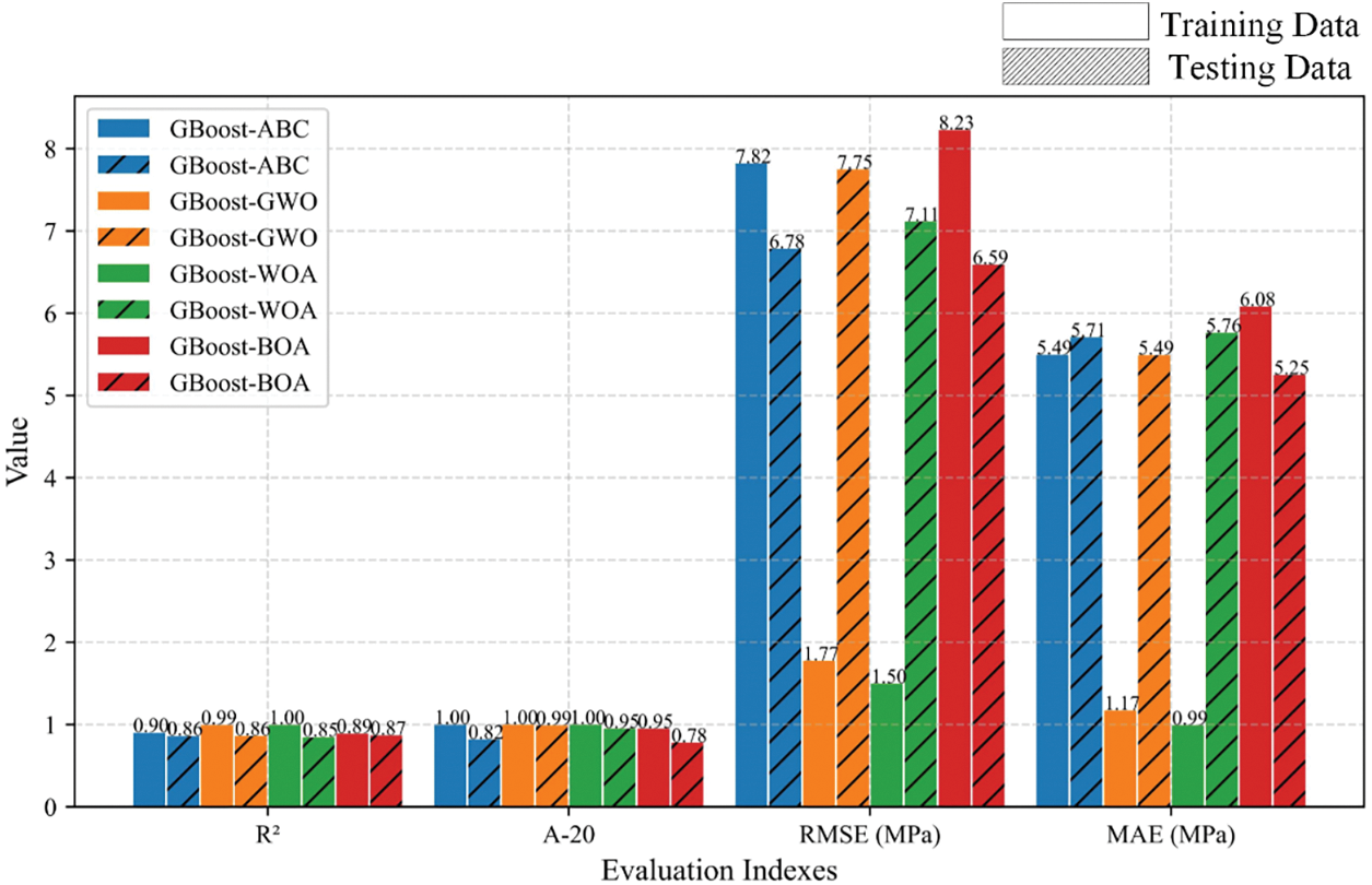
Figure 16: Comparison results of the prediction performance of the AdaBoost hybrid models
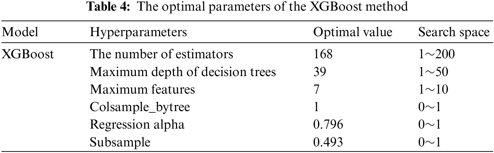
5.3 Development of the XGBoost Model
Finally, the hyperparameters of the XGBoost method, such as the number of estimators, maximum decision tree depth, maximum features, tree colsample, regression alpha, and subsample, were confirmed by using the four optimization methods. Figs. 17 and 18 show the corresponding training results for the hybrid models. The hybrid models XGBoost-ABC, XGBoost-GWO, and XGBoost-WOA obtained the best results at 35, 30, and 15 population sizes, respectively. The hybrid model XGBoost-BOA also performed robustly during the training process. Fig. 19 presents the prediction performance of each hybrid model on the training and testing datasets. The hybrid model XGBoost-ABC exhibited the strongest robustness on both training and testing data, with the evaluation index
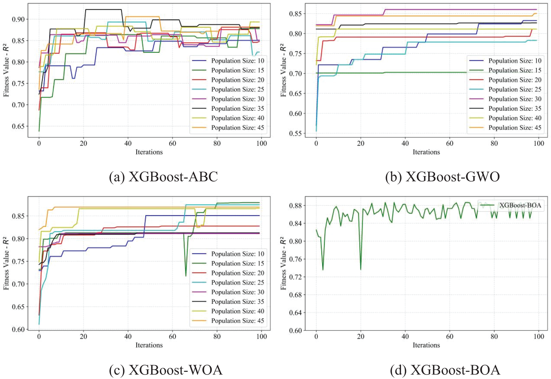
Figure 17: Fitness values of R2 of the XGBoost model using four optimization methods, ABC, GWO, WOA, and BOA, respectively
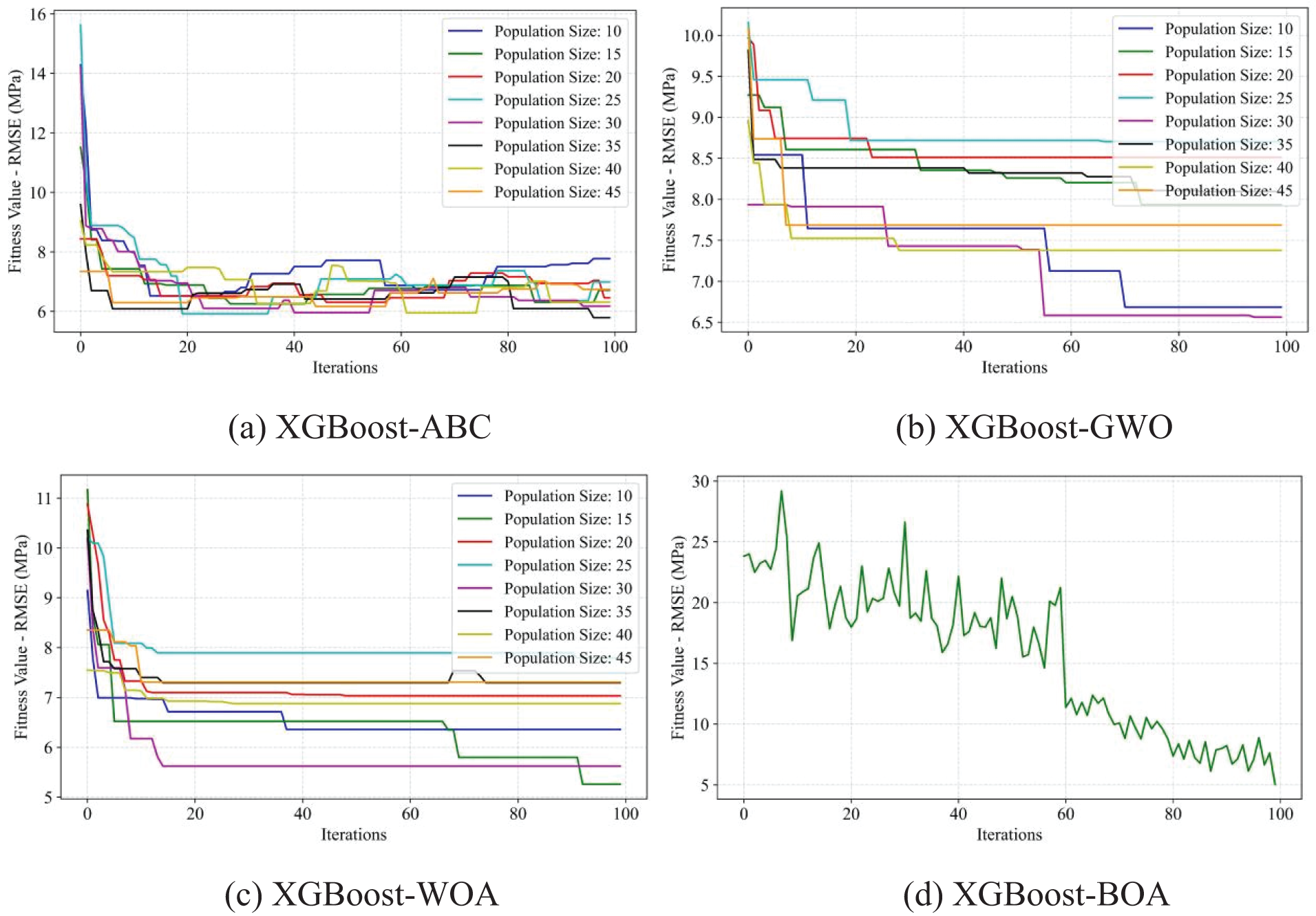
Figure 18: Fitness values of RMSE of the XGBoost model using four optimization methods, ABC, GWO, WOA, and BOA, respectively
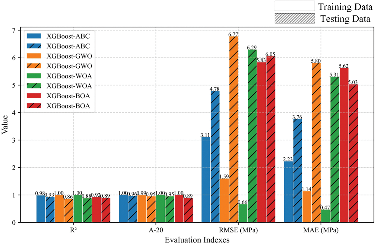
Figure 19: Comparison results of the prediction performance of the AdaBoost hybrid models
6 Model Prediction Performance Analysis and Discussion
Taylor diagrams [70] were employed to discuss the predictive model’s performance on the training and testing datasets. In Fig. 20, the markers indicate different models; the radial direction represents the correlation coefficient; the X-axis indicates the standard deviation, unnormalized; and the green dotted curves reflect the centered RMSE. The reference point with a black Pentastar indicates the actual UCS and other markers closer to this point denote better performance. The hybrid AdaBoost models show poor performance on both training and testing datasets. The hybrid GBoost and XGBoost models achieve acceptable results on the training datasets. However, hybrid XGBoost models perform better in the testing stage than GBoost models. In summary, XGBoost-ABC performs best compared to XGBoost-GWO, XGBoost-WOA, and XGBoost-BOA.
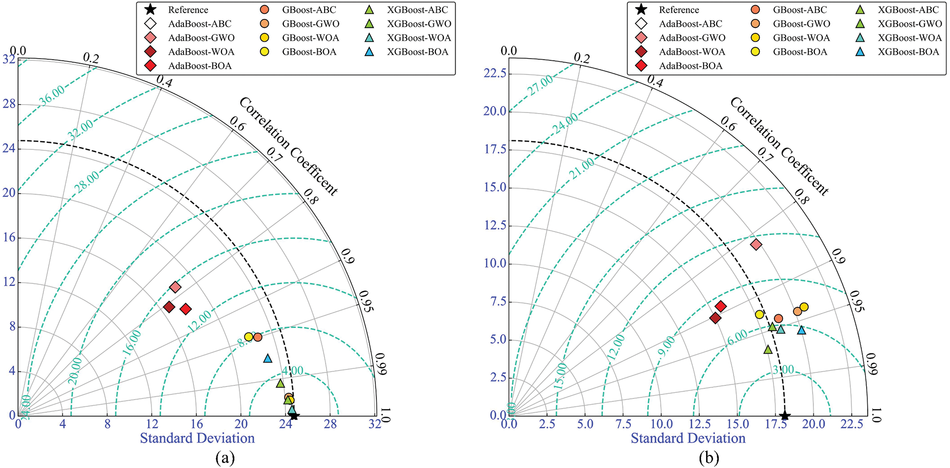
Figure 20: Taylor diagram. (a) Training data, (b) Testing data
Fig. 21 shows the prediction performance comparison of the optimal hybrid model for each boosting method. The results of the three evaluation indices for AdaBoost-ABC and GBoost-BOA are 0.60, 11.45, and 10.30 MPa; 0.87, 6.59, and 5.25 MPa, respectively. The XGBoost-ABC hybrid model achieved the highest R2 = 0.93 and the smallest RMSE and MAE (4.78 MPa and 3.76 MPa). The UCS prediction results of the hybrid model XGBoost-ABC on the testing dataset are shown in Fig. 22, where the red solid line represents the model prediction results, and the blue dotted line indicates the measured values.
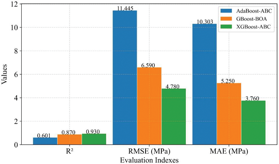
Figure 21: The performance comparison of the optimal hybrid model for each boosting method
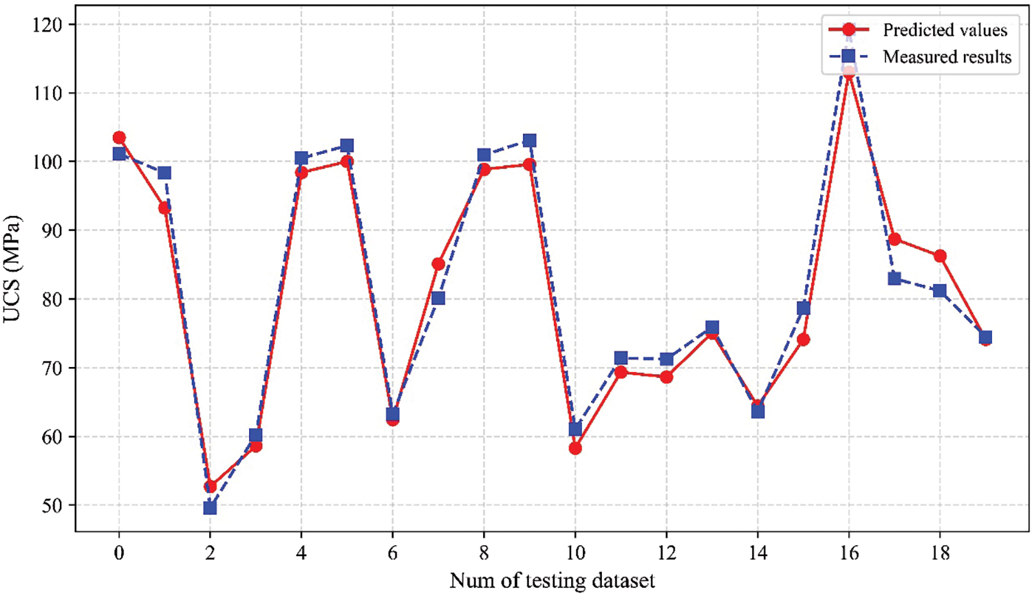
Figure 22: The prediction results of the hybrid XGBoost-ABC model on the testing dataset
Sensitivity analysis was employed to better understand the intrinsic relationships between the selected independent variables and rock UCS. The relevancy factor, a commonly used method to illustrate the sensitivity scale [71,72], was applied in this paper to assess the effect of each variable on UCS. The greater the absolute value of the relevancy factor between the independent and dependent variables, the stronger the influence. The calculation process of the sensitivity relevancy factor (SRF) is as follows:
where
The results showed that the most influential parameter on the UCS is the point load strength index (
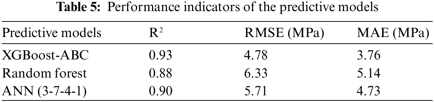
On the other hand, other intelligent algorithms, including random forest and artificial neural network (ANN), were trained with the same datasets to verify the superiority of the XGBoost-ABC model. The ANN model structure was 3-7-4-1, i.e., two hidden layers with 7 and 4 neurons, respectively. The prediction results of the two models are shown in Fig. 23, and the comparison results between the hybrid model XGBoost-ABC are presented in Table 5. The results demonstrate that the hybrid model XGBoost-ABC proposed in this paper performs better.
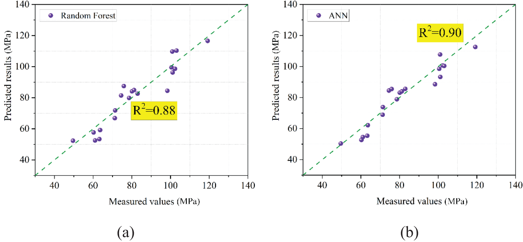
Figure 23: Performance of the random forest and ANN models using testing datasets. (a) is the prediction result of the random forest model, (b) is the prediction result of the ANN model
Based on the findings mentioned above, the proposed model XGBoost-ABC achieved an acceptable UCS prediction result. Fig. 24 presents the developed Graphical User Interface (GUI), which engineers can use as a portable tool to estimate the UCS of rock materials in deep mines. Nevertheless, it is essential to note that the developed model in this study is designed to address UCS prediction of rock in deep mining environments with three parameters: rock density, P-wave velocity, and point load strength.
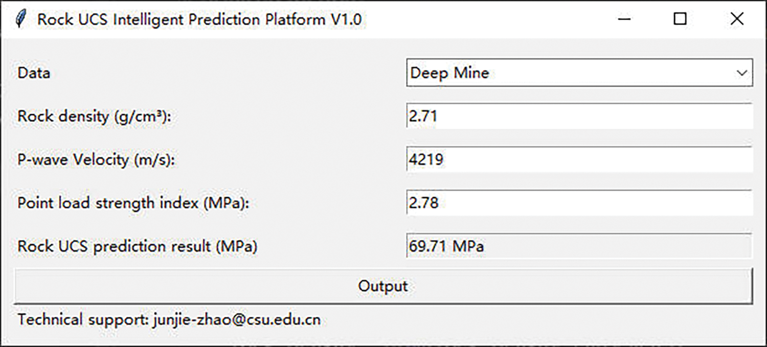
Figure 24: GUI for the prediction of rock UCS
In this research, a total of 106 samples are employed to investigate the mechanical properties of rocks in underground mines. Among them, 40 sets of data are taken from a deep lead-zinc mine in Southwest China, which can be regarded as a valuable database for investigating the mechanical properties of rocks in deep underground engineering. Three boosting-based models and four optimization algorithms are implemented to develop intelligent models for rock UCS prediction based on the established dataset. Based on the comparison results, it was found that the proposed hybrid model XGBoost-ABC exhibited superior prediction performance compared to the other models, with the highest
Overall, the proposed hybrid model achieves promising prediction accuracy on the data presented in this study. However, it is suggested that the model be fine-tuned on other datasets to ensure model prediction accuracy. In addition, more real-world data can be supplemented to enhance the robustness of the model. Finally, other physical and mechanical parameters can also be considered to develop rock strength prediction models in the future.
Acknowledgement: The authors wish to express their appreciation to the reviewers for their helpful suggestions, which greatly improved the presentation of this paper.
Funding Statement: This research is supported by the National Natural Science Foundation of China (Grant No. 52374153).
Author Contributions: Junjie Zhao: Writing–original draft, coding, model training. Diyuan Li: Supervision, writing review. Jingtai Jiang, Pingkuang Luo: Data collection and process. All authors reviewed the results and approved the final version of the manuscript.
Availability of Data and Materials: The datasets are available from the corresponding author upon reasonable request. https://github.com/cs-heibao/UCS_Prediction_GUI.
Conflicts of Interest: The authors declare that they have no conflicts of interest to report regarding the present study.
References
1. ISRM. (1981). Rock characterization testing and monitoring. ISRM suggested methods. Oxford: Pergamon Press. [Google Scholar]
2. ASTM (1986). Standard test method of unconfined compressive strength of intact rock core specimens. ASTM Standard. 04.08 (D 2938). [Google Scholar]
3. Jamshidi, A. (2022). A comparative study of point load index test procedures in predicting the uniaxial compressive strength of sandstones. Rock Mechanics and Rock Engineering, 55(7), 4507–4516. [Google Scholar]
4. Cao, J., Gao, J., Nikafshan Rad, H., Mohammed, A. S., Hasanipanah, M. et al. (2022). A novel systematic and evolved approach based on xgboost-firefly algorithm to predict young’s modulus and unconfined compressive strength of rock. Engineering with Computers, 38(5), 3829–3845. [Google Scholar]
5. Azimian, A., Ajalloeian, R., Fatehi, L. (2014). An empirical correlation of uniaxial compressive strength with P-wave velocity and point load strength index on marly rocks using statistical method. Geotechnical and Geological Engineering, 32, 205–214. [Google Scholar]
6. Barzegar, R., Sattarpour, M., Deo, R., Fijani, E., Adamowski, J. (2020). An ensemble tree-based machine learning model for predicting the uniaxial compressive strength of travertine rocks. Neural Computing and Applications, 32, 9065–9080. [Google Scholar]
7. Yılmaz, I., Sendır, H. (2002). Correlation of schmidt hardness with unconfined compressive strength and Young’s modulus in gypsum from Sivas (Turkey). Engineering Geology, 66(3–4), 211–219. [Google Scholar]
8. Kahraman, S. A. I. R., Gunaydin, O., Fener, M. (2005). The effect of porosity on the relation between uniaxial compressive strength and point load index. International Journal of Rock Mechanics and Mining Sciences, 42(4), 584–589. [Google Scholar]
9. Fener, M. U. S. T. A. F. A., Kahraman, S. A. İ. R., Bilgil, A., Gunaydin, O. (2005). A comparative evaluation of indirect methods to estimate the compressive strength of rocks. Rock Mechanics and Rock Engineering, 38, 329–343. [Google Scholar]
10. Yaşar, E., Erdoğan, Y. (2004). Estimation of rock physicomechanical properties using hardness methods. Engineering Geology, 71(3–4), 281–288. [Google Scholar]
11. Yilmaz, I. (2009). A new testing method for indirect determination of the unconfined compressive strength of rocks. International Journal of Rock Mechanics and Mining Sciences, 46(8), 1349–1357. [Google Scholar]
12. Basu, A., Kamran, M. (2010). Point load test on schistose rocks and its applicability in predicting uniaxial compressive strength. International Journal of Rock Mechanics and Mining Sciences, 47(5), 823–828. [Google Scholar]
13. Khandelwal, M. (2013). Correlating P-wave velocity with the physico-mechanical properties of different rocks. Pure and Applied Geophysics, 170, 507–514. [Google Scholar]
14. Amirkiyaei, V., Ghasemi, E., Faramarzi, L. (2021). Estimating uniaxial compressive strength of carbonate building stones based on some intact stone properties after deterioration by freeze–thaw. Environmental Earth Sciences, 80(9), 352. [Google Scholar]
15. Yagiz, S. (2009). Predicting uniaxial compressive strength, modulus of elasticity and index properties of rocks using the Schmidt hammer. Bulletin of Engineering Geology and the Environment, 68, 55–63. [Google Scholar]
16. Nazir, R., Momeni, E., Armaghani, D. J., Amin, M. F. M. (2013). Prediction of unconfined compressive strength of limestone rock samples using L-type Schmidt hammer. Electronic Journal of Geotechnical Engineering, 18, 1767–1775. [Google Scholar]
17. Wang, M., Wan, W. (2019). A new empirical formula for evaluating uniaxial compressive strength using the schmidt hammer test. International Journal of Rock Mechanics and Mining Sciences, 123, 104094. [Google Scholar]
18. Minaeian, B., Ahangari, K. (2013). Estimation of uniaxial compressive strength based on P-wave and Schmidt hammer rebound using statistical method. Arabian Journal of Geosciences, 6, 1925–1931. [Google Scholar]
19. Farhadian, A., Ghasemi, E., Hoseinie, S. H., Bagherpour, R. (2022). Prediction of rock abrasivity index (RAI) and uniaxial compressive strength (UCS) of granite building stones using nondestructive tests. Geotechnical and Geological Engineering, 40(6), 3343–3356. [Google Scholar]
20. Mishra, D. A., Basu, A. (2013). Estimation of uniaxial compressive strength of rock materials by index tests using regression analysis and fuzzy inference system. Engineering Geology, 160, 54–68. [Google Scholar]
21. Zhu, J., Chang, X., Zhang, X., Su, Y., Long, X. (2022). A novel method for the reconstruction of road profiles from measured vehicle responses based on the Kalman filter method. Computer Modeling in Engineering & Sciences, 130(3), 1719–1735. https://doi.org/10.32604/cmes.2022.019140 [Google Scholar] [CrossRef]
22. Chen, Q., Xu, C., Zou, B., Luo, Z., Xu, C. et al. (2023). Earth pressure of the trapdoor problem using three-dimensional discrete element method. Computer Modeling in Engineering & Sciences, 135(2), 1503–1520. https://doi.org/10.32604/cmes.2022.022823 [Google Scholar] [CrossRef]
23. Ghasemi, E., Gholizadeh, H. (2019). Prediction of squeezing potential in tunneling projects using data mining-based techniques. Geotechnical and Geological Engineering, 37, 1523–1532. [Google Scholar]
24. Kadkhodaei, M. H., Ghasemi, E., Mahdavi, S. (2023). Modelling tunnel squeezing using gene expression programming: A case study. Proceedings of the Institution of Civil Engineers-Geotechnical Engineering, 176(6), 567–581. [Google Scholar]
25. Liu, Z. D., Li, D. Y. (2023). Intelligent hybrid model to classify failure modes of overstressed rock masses in deep engineering. Journal of Central South University, 30(1), 156–174. [Google Scholar]
26. Li, D., Zhao, J., Liu, Z. (2022). A novel method of multitype hybrid rock lithology classification based on convolutional neural networks. Sensors, 22(4), 1574. [Google Scholar] [PubMed]
27. Li, D., Zhao, J., Ma, J. (2022). Experimental studies on rock thin-section image classification by deep learning-based approaches. Mathematics, 10(13), 2317. [Google Scholar]
28. Kadkhodaei, M. H., Ghasemi, E., Sari, M. (2022). Stochastic assessment of rockburst potential in underground spaces using Monte Carlo simulation. Environmental Earth Sciences, 81(18), 447. [Google Scholar]
29. Kadkhodaei, M. H., Ghasemi, E. (2022). Development of a semi-quantitative framework to assess rockburst risk using risk matrix and logistic model tree. Geotechnical and Geological Engineering, 40(7), 3669–3685. [Google Scholar]
30. Ghasemi, E., Gholizadeh, H., Adoko, A. C. (2020). Evaluation of rockburst occurrence and intensity in underground structures using decision tree approach. Engineering with Computers, 36, 213–225. [Google Scholar]
31. Ghasemi, E., Kalhori, H., Bagherpour, R., Yagiz, S. (2018). Model tree approach for predicting uniaxial compressive strength and Young’s modulus of carbonate rocks. Bulletin of Engineering Geology and the Environment, 77, 331–343. [Google Scholar]
32. Wang, M., Wan, W., Zhao, Y. (2020). Prediction of uniaxial compressive strength of rocks from simple index tests using random forest predictive model. Comptes Rendus Mecanique, 348(1), 3–32. [Google Scholar]
33. Jin, X., Zhao, R., Ma, Y. (2022). Application of a hybrid machine learning model for the prediction of compressive strength and elastic modulus of rocks. Minerals, 12(12), 1506. [Google Scholar]
34. Saedi, B., Mohammadi, S. D., Shahbazi, H. (2019). Application of fuzzy inference system to predict uniaxial compressive strength and elastic modulus of migmatites. Environmental Earth Sciences, 78, 1–14. [Google Scholar]
35. Li, J., Li, C., Zhang, S. (2022). Application of six metaheuristic optimization algorithms and random forest in the uniaxial compressive strength of rock prediction. Applied Soft Computing, 131, 109729. [Google Scholar]
36. Mahmoodzadeh, A., Mohammadi, M., Ibrahim, H. H., Abdulhamid, S. N., Salim, S. G. et al. (2021). Artificial intelligence forecasting models of uniaxial compressive strength. Transportation Geotechnics, 27, 100499. [Google Scholar]
37. Skentou, A. D., Bardhan, A., Mamou, A., Lemonis, M. E., Kumar, G. et al. (2023). Closed-form equation for estimating unconfined compressive strength of granite from three nondestructive tests using soft computing models. Rock Mechanics and Rock Engineering, 56(1), 487–514. [Google Scholar]
38. Liu, Q., Wang, X., Huang, X., Yin, X. (2020). Prediction model of rock mass class using classification and regression tree integrated AdaBoost algorithm based on TBM driving data. Tunnelling and Underground Space Technology, 106, 103595. [Google Scholar]
39. Wang, S. M., Zhou, J., Li, C. Q., Armaghani, D. J., Li, X. B. et al. (2021). Rockburst prediction in hard rock mines developing bagging and boosting tree-based ensemble techniques. Journal of Central South University, 28(2), 527–542. [Google Scholar]
40. Liu, Z., Armaghani, D. J., Fakharian, P., Li, D., Ulrikh, D. V. et al. (2022). Rock strength estimation using several tree-based ML techniques. Computer Modeling in Engineering & Sciences, 133(3), 799–824. https://doi.org/10.32604/cmes.2022.021165 [Google Scholar] [CrossRef]
41. Liu, Z., Li, D., Liu, Y., Yang, B., Zhang, Z. X. (2023). Prediction of uniaxial compressive strength of rock based on lithology using stacking models. Rock Mechanics Bulletin, 2(4), 100081. [Google Scholar]
42. Zhang, Q., Hu, W., Liu, Z., Tan, J. (2020). TBM performance prediction with Bayesian optimization and automated machine learning. Tunnelling and Underground Space Technology, 103, 103493. [Google Scholar]
43. Chen, T., Guestrin, C. (2016). Xgboost: A scalable tree boosting system. Proceedings of the 22nd ACM Sigkdd International Conference on Knowledge Discovery and Data Mining, pp. 785–794. San Francisco, CA, USA. [Google Scholar]
44. Ke, G., Meng, Q., Finley, T., Wang, T., Chen, W. et al. (2017). Lightgbm: A highly efficient gradient boosting decision tree. Proceedings of the Advances in Neural Information Processing Systems, pp. 3147–3155. Long Beach, CA, USA. [Google Scholar]
45. Prokhorenkova, L., Gusev, G., Vorobev, A., Dorogush, A. V., Gulin, A. (2018). CatBoost: Unbiased boosting with categorical features. Proceedings of the 32nd International Conference on Neural Information Processing Systems, vol. 31, pp. 6638–6648. Montréal, QC, Canada. [Google Scholar]
46. Chen, T., He, T., Benesty, M., Khotilovich, V., Tang, Y. et al. (2015). xgboost: eXtreme gradient boosting. R Package Version 0.4-2, 1(4), 1–4. [Google Scholar]
47. Chang, Y. C., Chang, K. H., Wu, G. J. (2018). Application of eXtreme gradient boosting trees in the construction of credit risk assessment models for financial institutions. Applied Soft Computing, 73, 914–920. [Google Scholar]
48. Zhang, W., Wu, C., Zhong, H., Li, Y., Wang, L. (2021). Prediction of undrained shear strength using extreme gradient boosting and random forest based on Bayesian optimization. Geoscience Frontiers, 12(1), 469–477. [Google Scholar]
49. Nguyen-Sy, T., Wakim, J., To, Q. D., Vu, M. N., Nguyen, T. D. et al. (2020). Predicting the compressive strength of concrete from its compositions and age using the extreme gradient boosting method. Construction and Building Materials, 260, 119757. [Google Scholar]
50. Pelikan, M., Goldberg, D. E., Cantú-Paz, E. (1999). BOA: The Bayesian optimization algorithm. Proceedings of the Genetic and Evolutionary Computation Conference GECCO-99, vol. 1, pp. 525–532. Orlando, FL, USA. [Google Scholar]
51. Díaz, E., Salamanca-Medina, E. L., Tomás, R. (2023). Assessment of compressive strength of jet grouting by machine learning. Journal of Rock Mechanics and Geotechnical Engineering, 16, 102–111. [Google Scholar]
52. Lahmiri, S., Bekiros, S., Avdoulas, C. (2023). A comparative assessment of machine learning methods for predicting housing prices using Bayesian optimization. Decision Analytics Journal, 6, 100166. [Google Scholar]
53. Bo, Y., Huang, X., Pan, Y., Feng, Y., Deng, P. et al. (2023). Robust model for tunnel squeezing using Bayesian optimized classifiers with partially missing database. Underground Space, 10, 91–117. [Google Scholar]
54. Díaz, E., Spagnoli, G. (2023). Gradient boosting trees with Bayesian optimization to predict activity from other geotechnical parameters. Marine Georesources & Geotechnology, 1–11. [Google Scholar]
55. Greenhill, S., Rana, S., Gupta, S., Vellanki, P., Venkatesh, S. (2020). Bayesian optimization for adaptive experimental design: A review. IEEE Access, 8, 13937–13948. [Google Scholar]
56. Karaboga, D. (2005). An idea based on honey bee swarm for numerical optimization. In: Technical report-TR06, Erciyes University, Engineering Faculty, Computer Engineering Department. [Google Scholar]
57. Bharti, K. K., Singh, P. K. (2016). Chaotic gradient artificial bee colony for text clustering. Soft Computing, 20, 1113–1126. [Google Scholar]
58. Asteris, P. G., Nikoo, M. (2019). Artificial bee colony-based neural network for the prediction of the fundamental period of infilled frame structures. Neural Computing and Applications, 31(9), 4837–4847. [Google Scholar]
59. Parsajoo, M., Armaghani, D. J., Asteris, P. G. (2022). A precise neuro-fuzzy model enhanced by artificial bee colony techniques for assessment of rock brittleness index. Neural Computing and Applications, 34, 3263–3281. [Google Scholar]
60. Zhou, J., Koopialipoor, M., Li, E., Armaghani, D. J. (2020). Prediction of rockburst risk in underground projects developing a neuro-bee intelligent system. Bulletin of Engineering Geology and the Environment, 79, 4265–4279. [Google Scholar]
61. Mirjalili, S., Mirjalili, S. M., Lewis, A. (2014). Grey wolf optimizer. Advances in Engineering Software, 69, 46–61. [Google Scholar]
62. Golafshani, E. M., Behnood, A., Arashpour, M. (2020). Predicting the compressive strength of normal and high-performance concretes using ANN and ANFIS hybridized with grey wolf optimizer. Construction and Building Materials, 232, 117266. [Google Scholar]
63. Shariati, M., Mafipour, M. S., Ghahremani, B., Azarhomayun, F., Ahmadi, M. et al. (2022). A novel hybrid extreme learning machine–grey wolf optimizer (ELM-GWO) model to predict compressive strength of concrete with partial replacements for cement. Engineering with Computers, 38, 757–779. [Google Scholar]
64. Mirjalili, S., Lewis, A. (2016). The whale optimization algorithm. Advances in Engineering Software, 95, 51–67. [Google Scholar]
65. Zhou, J., Zhu, S., Qiu, Y., Armaghani, D. J., Zhou, A. et al. (2022). Predicting tunnel squeezing using support vector machine optimized by whale optimization algorithm. Acta Geotechnica, 17(4), 1343–1366. [Google Scholar]
66. Tien Bui, D., Abdullahi, M. A. M., Ghareh, S., Moayedi, H., Nguyen, H. (2021). Fine-tuning of neural computing using whale optimization algorithm for predicting compressive strength of concrete. Engineering with Computers, 37, 701–712. [Google Scholar]
67. Nguyen, H., Bui, X. N., Choi, Y., Lee, C. W., Armaghani, D. J. (2021). A novel combination of whale optimization algorithm and support vector machine with different kernel functions for prediction of blasting-induced fly-rock in quarry mines. Natural Resources Research, 30, 191–207. [Google Scholar]
68. Momeni, E., Armaghani, D. J., Hajihassani, M., Amin, M. F. M. (2015). Prediction of uniaxial compressive strength of rock samples using hybrid particle swarm optimization-based artificial neural networks. Measurement, 60, 50–63. [Google Scholar]
69. Lei, Y., Zhou, S., Luo, X., Niu, S., Jiang, N. (2022). A comparative study of six hybrid prediction models for uniaxial compressive strength of rock based on swarm intelligence optimization algorithms. Frontiers in Earth Science, 10, 930130. [Google Scholar]
70. Taylor, K. E. (2001). Summarizing multiple aspects of model performance in a single diagram. Journal of Geophysical Research: Atmospheres, 106, 7183–7192. [Google Scholar]
71. Chen, G., Fu, K., Liang, Z., Sema, T., Li, C. et al. (2014). The genetic algorithm based back propagation neural network for MMP prediction in CO2-EOR process. Fuel, 126, 202–212. [Google Scholar]
72. Bayat, P., Monjezi, M., Mehrdanesh, A., Khandelwal, M. (2021). Blasting pattern optimization using gene expression programming and grasshopper optimization algorithm to minimise blast-induced ground vibrations. Engineering with Computers, 38, 3341–3350. [Google Scholar]
Cite This Article
 Copyright © 2024 The Author(s). Published by Tech Science Press.
This work is licensed under a Creative Commons Attribution 4.0 International License , which permits unrestricted use, distribution, and reproduction in any medium, provided the original work is properly cited.
 Downloads
 Citation Tools