Numerical Analysis of Perforation during Hydraulic Fracture Initiation Based on Continuous–Discontinuous Element Method

1  Introduction

Hydraulic fracturing is a pivotal technology to increase oil and gas production [1,2]. In engineering applications, directional hydraulic fracturing techniques are employed to establish the main channels in the wellbore [3]. A commonly used technique is to use a perforating bullet, as shown in Fig. 1. Perforation can not only reduce the injection pressure but also guide the direction of hydraulic fracture propagation, enhancing well production capacity and assisting mechanical excavation for hard rock mass in underground engineering [4–7]. Breakdown pressure signifies the resistance to rock mass fracturing, playing a pivotal role in determining fracture gradients in drilling, designing perforation fracturing schemes, analyzing wellbore pressure evolution, and assessing wellbore compliance [8–10]. Various types of perforating bullets result in distinct perforation channel configurations, which in turn affect breakdown pressures and rock fracture degree.

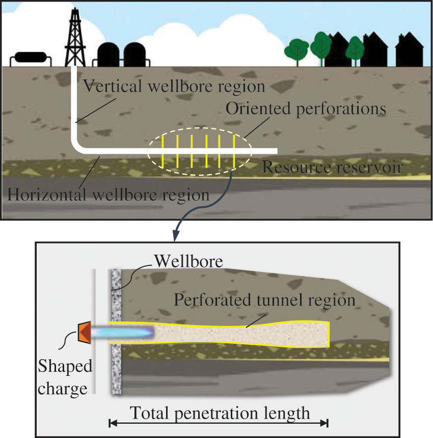
Figure 1: Diagram of directional perforating technique and perforating charge channel

Certain researchers conduct hydraulic fracturing experiments incorporating perforations. For instance, Behrmann et al. [11] acquired perforation geometry by using perforating guns and assessed the breakdown pressures using a triaxial stress cell. Abass et al. [12] induced a single wide fracture through directional perforation testing. Zhang et al. [13] conducted large-scale true triaxial hydraulic fracturing experiments in cubic rock samples, analyzing the fracture distribution of perforations and breakdown pressures. Zheng et al. [14] investigated the effect of pore pressure on breakdown pressure by true triaxial test. Zhai et al. [15] illustrated the effect of in-plane perforation using a large installation. Without the cost and hardware limitations of experiments, numerical studies offer a convenient means of obtaining results for perforating fractures.

Compared to experimental investigations, numerical methods are more efficient and flexible. Various numerical methods have been proposed to simulate the fracture propagation, including the extended finite element method (XFEM) [16–18], generalized finite element method (GFEM) [19], discrete element method (DEM) [20,21], discontinuous deformation analysis (DDA) [22] and cohesive zone method (CZM) [23], displacement discontinuity method (DDM) [24], gradient damage model [25], and phase field model (PFM) [26,27]. These methods represent advancements in traditional finite element or discrete element approaches. Additionally, other methods include the cracking elements method [28–30] based on the finite element method, peridynamics [31,32], the combined finite-discrete element method (FDEM) [33,34], general particle dynamics [35], field enriched finite element method [36] and the continuous–discontinuous element method (CDEM) [37–39], among others. The continuous–discontinuous element method, in comparison with other methods, amalgamates the attributes of finite element and discrete element methodologies, and can better simulate the deformation of solids [40], the expansion of cracks under thermal action [41], and the flow and diffusion of fluid matrix in cracks [42–44].

The simulations on perforation fracturing explore various key factors, such as perforation parameters (perforation angle, density, length), formation mechanical parameters (rock properties, in-situ stress difference), and fracturing parameters (flow rate, fluid viscosity) [45–47]. Some studies simplify wellbore and perforation into two-dimensional models, where perforation channels are substituted by pre-existing fissures [48–52]. Recently, researchers have employed fully three-dimensional models to investigate the perforation process. Zhao et al. [53] utilized FRANC3D to construct a three-dimensional cylindrical perforation model and examined the influence of various spatial arrangements of perforations on hydraulic fracture propagation. Shan et al. [54] developed a three-dimensional model using the finite element method (FEM) to investigate the expansion of horizontal well fractures. Wanniarachchi et al. [55] utilized the COMSOL Simulator to construct a three-dimensional horizontal well model to investigate the impact of perforation spacing. The results indicated that reducing the perforation spacing leads to an increase in overall strain levels. Dong et al. [56] employed the CZM to simulate the multi-angle perforation fracturing process under triaxial stress conditions and pointed out that perforation in vertical orientation was more likely to fracture. Huang et al. [57] studied the stress competition mechanism under three-dimensional multiple perforation conditions using the 3D Lattice Method. In addition to creating 3D physical models, researchers have integrated physical models with data-driven models not only to study the fracturing process but also to optimize pumping schedules [58,59].

Previous studies have primarily simplified perforations as an ideal cylindrical shape, often overlooking the actual non-uniformity of perforation geometries. To the best of our knowledge, no investigation has been carried out to discuss the influence of specific perforation shapes on the effects of hydraulic fracturing while the created perforations are not perfectly regular cylindrical boreholes in practical engineering. In this study, the borehole shape characteristics and dimensions of four commonly used perforations are obtained based on engineering reports. With a hybrid finite-discrete element method known as CDEM [37–39], a model coupling hydraulic fracturing with perforation is created, providing a detailed representation of the four types of perforations, with some simulation parameters calibrated through experimental validation. Then the model was used to select the optimal perforation type. Subsequently, the study explored the impact of perforation shape parameters (cross-sectional diameter and penetration length) on the fracturing effectiveness.

2  Continuous−Discontinuous Element Method (CDEM)

2.1 The Basic Concept of CDEM

The CDEM is an explicit computational method that combines the FEM and the DEM [37–39]. FEM is utilized for computing the stress field, including node velocity and acceleration, node displacement, and node force. DEM is employed for calculating fracture network, which involves calculating spring force, applying fracture criteria for fracture assessment, and calculating fracture aperture. The theoretical foundation of CDEM is Lagrange’s equation, expressed by Eq. (1) [40–43].

ddt(∂L∂u˙i)−∂L∂ui=Qi(1)

where ui is the generalized coordinate, and u˙i is the temporal derivative of the generalized coordinate. Qi is the generalized non-conservative force. L is the Lagrange function, which can be expressed by Eq. (2).

L=Πm+Πe+Πf(2)

where Πm, Πe and Πf are the kinetic energy, elastic energy, and potential energy of the system, respectively.

The governing equations for CDEM are represented by Eq. (3).

Mu¨+Cu˙+Ku+Kcuc+Ccu˙c=Fe(3)

where M represents the concentrated mass matrix. C is the damping matrix. K is the element stiffness matrix. Kc is the element stiffness matrix of the contact surface. Cc is the damping matrix of the contact surface. Fe is the element external force vector, including the solid force and fluid pressure. u¨, u˙ and u are the acceleration, velocity, and displacement matrices of the nodes of block elements. uc and u˙c are relative displacement arrays and relative velocity arrays on virtual interface nodes.

In the time domain, Euler’s forward difference method is used for explicit iterative solutions in CDEM, and the difference form is expressed by Eq. (4).

{u˙n+1=u˙n+u¨nΔtun+1=un+u˙n+1Δt(4)

where n is the number of iteration steps and Δt represents a time step.

CDEM consists of two components: the block model and the contact model. The block model represents the material’s continuous properties, while the contact model encompasses real and virtual contact surfaces to characterize discontinuous behaviors such as material fracture and sliding. The composition of CDEM elements is illustrated in Fig. 2. The interfaces between block elements represent joints and faults within the rock mass and are depicted by real contact surfaces. Each block element consists of one or more units interconnected by virtual contact surfaces, which provide fracture pathways when damage occurs in the continuous part of the rock mass. Virtual normal and tangential contact springs connect the contact surfaces, and the failure of these springs signifies the transition from continuous to discontinuous material failure processes.

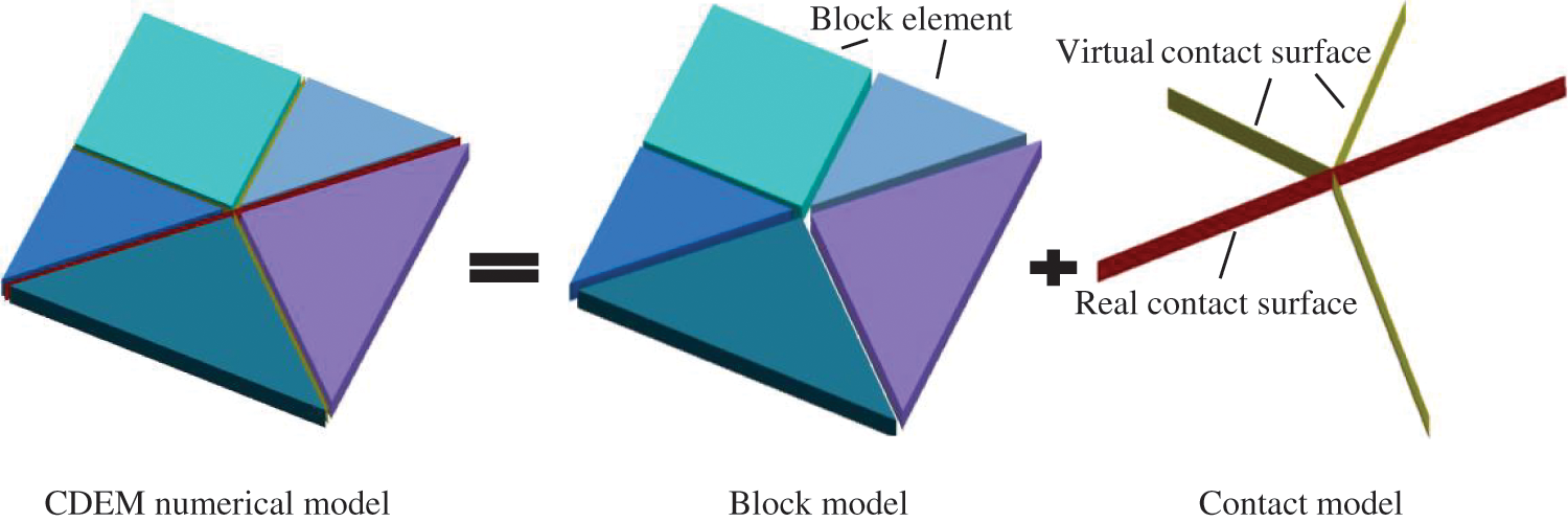
Figure 2: Basic concept of CDEM

The stress-strain relationship and geometric relationship between the blocks are expressed by Eq. (5).

{σ=D:εε=12(u∇+∇u)(5)

where σ is the stress tensor. ε is the strain tensor. D is an elastic matrix.

2.2 Material Constitutive Relation and Failure Criteria

The constitutive behavior of the block elements is characterized by linear elasticity, and an incremental approach [38] is used to calculate the element stresses, representing the linear elastic constitutive model as shown in Eq. (6).

{Δσij=2GΔεij+(K−23G)Δθδijσij(t)=Δσij+σij(t−Δt)(6)

where Δσij denotes the stress increment at the current time step. Δεij represents the strain increment at the current time step. Δθ refers to the volumetric strain increment at the current time step. K is the bulk modulus (Pa). G is the shear modulus (Pa). δij stands for the Kronecker delta symbol. σij(t) represents the stress at the current time step (Pa). σij(t−Δt) represents the stress at the previous time step (Pa).

Mohr-Coulomb constitutive modeling of brittle fracture is employed for these contact surfaces, and the occurrence of failure is determined using the maximum tensile stress criterion. The calculation of contact forces for normal and tangential springs is initially determined using Eq. (7).

{Fn(t+Δt)=Fn(t)−KnΔdnFs(t+Δt)=Fs(t)−KsΔds(7)

where Fn represents the normal contact force (N). Fs stands for the tangential contact force (N). Kn and Ks are the normal and tangential contact stiffness per element area (Pa/m). Δdn and Δds represent the normal and tangential relative displacement increments.

Eqs. (8) and (9) are employed to calculate tensile failure.

If

−Fn(t+Δt)≥T0Ac(8)

then

{Fn(t+Δt)=−T0AcT(t+Δt)=0(9)

Eqs. (10) and (11) are applied to determine shear failure.

If

Fs(t+Δt)≥Fn(t+Δt)tan⁡φc+c0Ac(10)

then

{Fs(t+Δt)=Fn(t+Δt)tan⁡φcC(t+Δt)=0(11)

where Fs(t+Δt) is the tangential contact force at the next time step (N). φc is the internal friction angle of the interface. c0 is the initial interface cohesion at the initial time step (Pa) and it becomes C(t+Δt) after failure.

2.3 Hydraulic Coupling Model

A model that describes fluid flowing along fractures is established. The coupling between solid and fracture seepage is achieved through the interaction between the contact surface and fracture seepage. Fracture seepage applies pressure on the contact surface between adjacent solids, and the deformation of the contact surface affects the fracture opening, which in turn affects fracture seepage. As depicted in Fig. 3, solid element A and the adjacent solid element B are connected by the fracture element. The diffusion of fluid generates fracture pressures on the two solid elements connected by the fracture element.

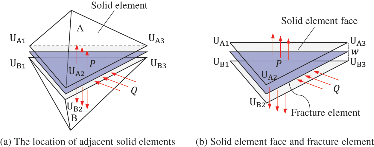
Figure 3: Diagram of hydraulic coupling between solid deformation and fracture seepage

As shown in Fig. 4, crack pressure and node saturation are assigned at the node location, while the flow rate is specified at the cell centroid.

Figure 4: Diagram of planar fracture elements

The change in relative displacement between two solid elements affects the opening of the fracture element. It is assumed that the permeability of the crack or joint follows the cubic law. According to Eq. (12), the fracture permeability varies with the change in fracture aperture, denoted as w. In CDEM, KE is employed as the permeability coefficient (m2/(Pa·s)), representing the permeability characteristics of the fracture.

KE=κμ=w212μ(12)

where κ is the permeability ratio (m2). μ is the dynamic viscosity of fluid (Pa·s).

The seepage in fracture follows Darcy’s law. According to Darcy’s Law, the fluid velocity of a node can be expressed by Eq. (13).

vi=−KEks∂PE∂xi(13)

where xi represents the coordinate component of the direction i of a node. PE represents the total nodal fluid pressure. ks represents the relative permeability coefficient, which can be expressed by Eq. (14).

ks=S¯2(3−2S¯)(14)

where S¯ represents the average saturation of fracture element, S¯=∑i=1nSi. Si represents the saturation of each node.

According to the Gaussian divergence theorem, Eq. (13) can be formulated into Eq. (15).

vi=KEks1V∑j=1MP¯jniΔSj(15)

where M is the total number of faces per fracture element. V is the element volume. ni represents the component of the jth face associated with the node in the direction i. P¯jrepresents the average value of the total pressure PE of the node in the jth face, and ΔSj is the jth face area.

The flow rate of each node is q, which can be calculated by Eq. (16).

q=∑j=1M(v⋅nj)ΔSjNj(16)

where v is the fluid velocity vector of the fracture element. nj is the element outer normal vector of jth face, Nj is the total number of nodes of the jth face.

The flow rate through each node of the fracture element, Q, can be given by Eq. (17).

Q=∑j=1Nqj(17)

where N represents the number of elements connected to this node.

The saturation of each node is calculated by node flow and is expressed by Eq. (18).

S=−∑t=0t(Q+QEnVΔt)(18)

where QE is the external flow boundary condition. n is the total number of nodes of the fracture element. V represents the element volume.

When the saturation of the node accumulates to 1, the total nodal fluid pressure PE can be given by Eq. (19).

PE=−∑t=0t(KwQ+QEnVΔt)−S¯ρw(xgx+ygy+zgz)(19)

where Kw is the bulk modulus of fluid, ρw represents the fluid density. gx, gy, gz are the global component of the acceleration of gravity, respectively. x, y, z represent the three components of the global coordinate of a node, respectively.

Subsequently, by incorporating the fluid pressure PE into Eq. (3), we can calculate the solid stress field and the discontinuous field, resulting in the updated nodal displacements of the solid elements (UAi, UBi, i = 1, 2, 3). The fracture aperture for each node is determined by Eq. (20). The coupling concept between the fluid and solid is shown in Fig. 5.

wi=|UAi−UBi|,i=1,2,3(20)

Figure 5: Mechanism of hydraulic coupling between solid and fluid

3  Numerical Model Validation

3.1 Fluid Driven Fracture Propagation Simulation

To verify the effectiveness of CDEM in simulating hydraulic fracturing processes in rocks, this section conducts simulations of the seepage process in rock matrices containing pre-existing horizontal fissure. The simulation validation scheme is designed based on reference [32], which utilized the peridynamic model to simulate the seepage process. The two-dimensional rock model with a horizontal pre-existing fissure is illustrated in Fig. 6a. The rock specimen is simplified into a two-dimensional square model with a side length of 1 m. A horizontal fissure is pre-set at the middle position of this model, with a length of 0.2 m. Water pressure is applied to the horizontal fissure to simulate the process of fluid expanding the crack. Under the assumption of plane strain, Sneddon et al. [60] proposed that the y-direction displacement uy of a single pre-existing fissure with a length of 2 lc on a two-dimensional plane driven by water pressure p can be expressed by Eq. (21). Consequently, the vertical displacement along the crack direction of the model can be calculated and then the numerical results can be verified against analytical solutions.

uy(x,p)=2plc(1−v2)E(1−x2lc2)12(21)

where x is the distance from the center of the pre-existing fissure (m). E is the elastic modulus of rock (GPa). v is the Poisson ratio of the rock.

Figure 6: Verification diagram of hydraulic driven crack propagation

Due to the low permeability of porous rock, this study only considers fracture seepage. The boundaries of the rock model are set as fixed permeable boundaries. The computational parameters of the rock are listed in Table 1. The model is divided into 5,000 triangular elements. Eleven monitoring points are evenly arranged at the position of the pre-existing fissure to monitor the simulated vertical displacement values. The analytical solution corresponds to a stable fracturing process. In this study, a constant water pressure of 22 MPa is applied over the entire pre-existing fissure. After 150,000 steps, convergence is reached, and displacement results are obtained.

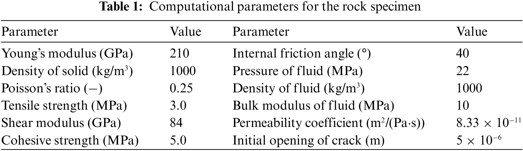
Fig. 6b compares the magnitude of vertical displacement between numerical simulation results and analytical solutions. The simulation results of CDEM closely align with the analytical solution and existing research results [32]. This indicates that CDEM can effectively simulate the process of fluid-driven fracture propagation.

3.2 Validation against Experimental Data

This section entails a comparison between numerical simulations with hydraulic fracturing experimental results, the calibration of distinct simulation parameters concerning distinct stress conditions and material properties, and the validation of the accuracy of the simulation results. Jiang et al. [61] conducted physical tests of directional perforation fracturing on a cubic specimen measuring 300 mm on each side, composed of a mixture of cement and quartz sand. This test simulated the perforation fracturing process under conditions involving three directional in-situ stresses and water pressure, yielding data on fracturing pressure and fracture morphology. Parameters provided by the test include the sample size, wellbore dimensions, perforation size and arrangement, and the three directions of in-situ stresses. These parameters can be used for parameter correction of numerical models. Detailed fracturing test parameters can be found in Table 2. Additionally, to ensure the reliability of the comparisons, a three-dimensional model was constructed based on the experimental parameters, as illustrated in Fig. 7.

Figure 7: Geometric diagram of the test model

A constant flow boundary condition is imposed at the termination of the perforation, a common practice in perforation fracturing simulations [5,51]. Owing to the low permeability of the sample material, the porous permeability of the block elements was disregarded in the simulation, with fluid flowing solely within fractures. Material parameters and the flow rates align with the experimental setup, and specific parameters are detailed in Table 3.

As shown in Fig. 8, a comparison is made between the numerical results (Figs. 8a to 8c) and experimental results (Figs. 8d and 8e) of directional symmetric perforation fracturing at the azimuth angle of 60°. The figure illustrates that the fractures propagate along the direction of perforation and deflect towards the direction of maximum principal stress, resulting in a curved fracture surface. Due to spatial overlap of fracture planes when viewed planarly, the cracks in Fig. 8b exhibit a banded appearance. Fig. 8c displays a fracture surface resembling that in Fig. 8e, clearly indicating the correspondence between numerical and experimental observations.

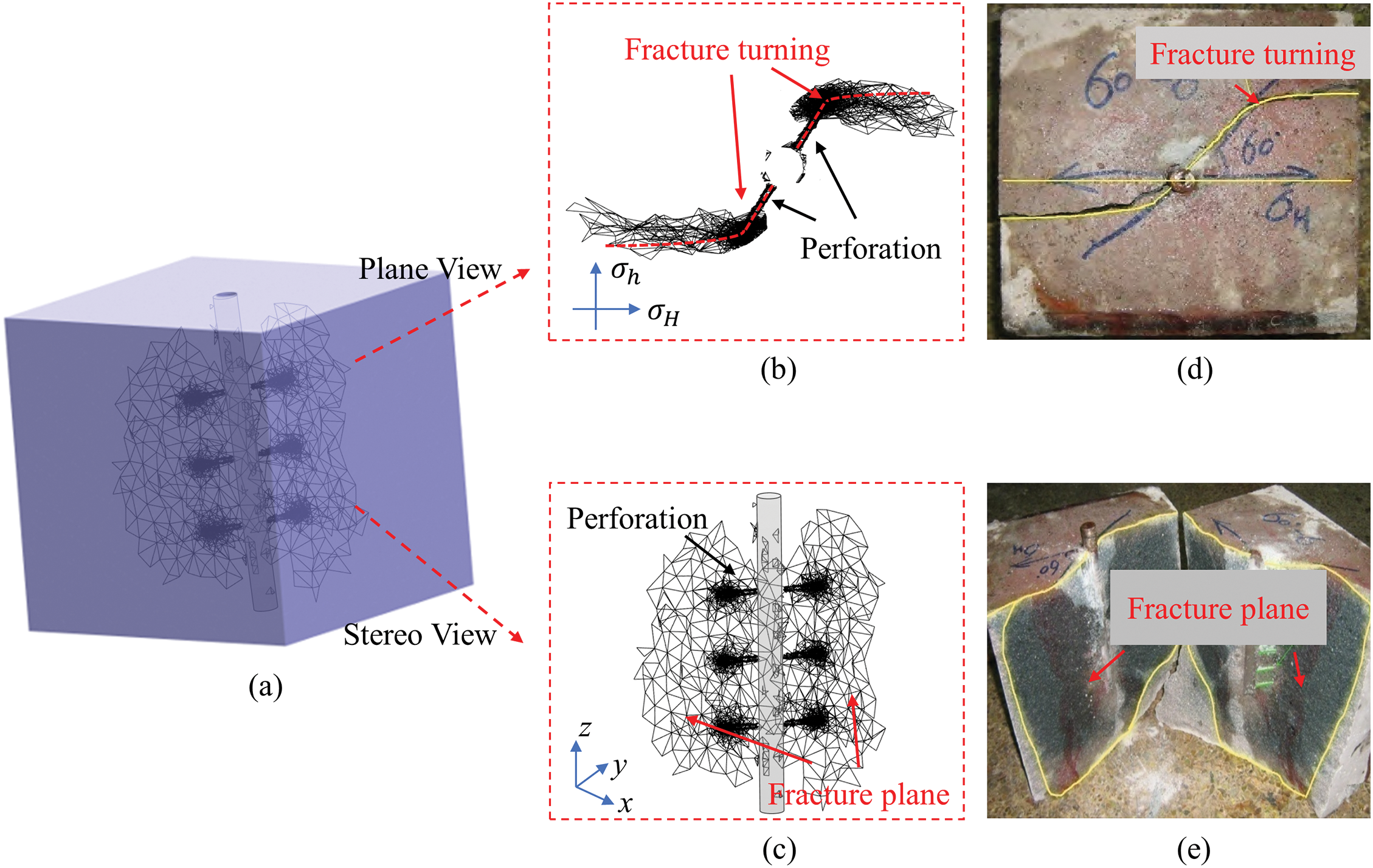
Figure 8: Comparison between simulation and physical test of perforation fracturing at the azimuth angle of 60°: (a)~(c) are simulation results, and (d)~(e) are test results [61]

Fig. 9 presents statistical data on water injection pressure, where the peak pressure at the wellhead signifies the breakdown pressure, which increases with the azimuth angle. When θ is 30°, 45°, and 60°, the simulated values are 10.46, 10.65, and 15.64 MPa, respectively. Correspondingly, the measured breakdown pressures for these angles are 10.39, 10.55, and 15.55 MPa, respectively [61]. The simulated breakdown pressures closely match the measured values, confirming the reliability of the present numerical model.

Figure 9: Validation of the simulation through comparison with experimental data

3.3 Validation against Field Data

This section contrasts the simulation outcomes with engineering data. While the material parameters align with those outlined in Section 3.2, there are notable differences in dimensions and in-situ stresses. Specifically, the specimen and perforation dimensions in the laboratory are considerably smaller than those encountered in the field. To validate the simulation capability, the field’s fracturing perforation results will be employed.

Sun et al. [62] presented field data on the perforation fracturing of Changqing Oilfield (Xi’an, China). In Fig. 10a, a 2 m cube is used to model the underground rock stratum, with a horizontal wellbore located in the center. While Sun et al. [62] did not specify the size of the wellbore, the radius is assumed to be 70 mm. The model features one perforation cluster with 6 perforations. Each perforation has a length of 400 mm, a diameter of 20 mm, and a spacing of 200 mm. The perforation phase angle is 60°, and the direction of the middle two perforations is consistent with that of σH. To accommodate for engineering factors, a larger flow rate is used compared to indoor tests. The simulation utilizes parameters similar to those outlined in Table 3, with discrepancies in other parameters detailed in Table 4.

Figure 10: Simulated fracturing results for engineering data validation

Figs. 10b to 10d present the results of the numerical simulation. In Fig. 10b, the initial crack originates from the base of the perforation at 7 s, consistent with the conclusion of Sun et al. [62]. At this moment, the tensile stress is primarily focused at the base of the perforation. The perforation root is located at the junction of the wellbore and perforation. Due to the large size gradient in the root area, stress concentration and crack initiation are easily produced. As shown in Figs. 10c and 10d, the simulated breakdown pressure of the spiral perforation is 44.26 MPa, compared to Sun’s 44.5 MPa and the field data’s 43.0 MPa, with differences of 2.93% and 3.49%, respectively. This underscores the model’s commendable simulation accuracy when handling high in-situ stresses and large perforation sizes.

4  Fracturing Simulation and Analysis

4.1 Acquisition of Real Perforation Shapes

Before analyzing perforating fracturing, it is essential to establish a perforation model. Real perforation data offer parameters for modeling of perforation, including perforation length, perforation diameter and shape characteristics. According to an engineering technical report, Figs. 11 and 12 illustrate the perforation effects and sizes of four types of penetration bullets in sandstone. These four types of penetrating bullets are: 25g DP3 HMX, 39g DP3 HMX, 89-type deep-penetrating perforating bullet (EH38RDX27-3), and 95-type deep-penetrating perforating bullet (213SD-95R-1HR).

Figure 11: Profile of four kinds of penetrating bullet through sandstone target

Figure 12: Size diagram of four kinds of penetrating bullets

Fig. 11 illustrates that all four types of perforations display different cross-sectional shapes. The evolution of cross-sectional changes is characterized by initial constriction followed by expansion. These perforations can be divided into two sections: a constricted section (near to the wellbore) and an expanded section (away from the wellbore). While the lengths of the constricted sections are similar for all four perforation types, the lengths of the expanded sections vary, leading to variations in penetration lengths. Moreover, there is notable diversity in the far-end radius among different perforations.

The variable cross-sectional dimensions of each perforation are depicted in Fig. 12a. In this figure, the perforations are numbered from left to right as 1, 2, 3, and 4, and the cross-sectional radii are marked at 50 mm intervals along the penetration length. Sections beyond these intervals are considered as separate segments, and detailed data on perforation length are presented in Table 5.

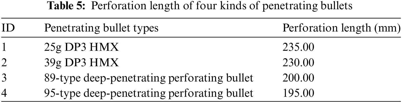
Fig. 12b utilizes Perforation No. 2 as an example. The perforation is divided into two segments by a specific position where the cross-sectional radius transitions from constricted to expanded (position d4). The segment nearer to the wellbore, with a length denoted as lN, is referred to as the near-well section. The segment away from the wellbore, with a length denoted as lD, is referred to as the far-well section. Each segment is subdivided into five subsections, labeled as l1 through l5.

4.2 Model Setup

The section diameter and length of the perforation model can be determined based on the dimensions of various perforations provided in Fig. 12. Fig. 13a displays the geometric model of the rock, which is a 2 m cube with a cylindrical component in the center simulating the wellbore, featuring a radius of 70 mm. The perforations are positioned on one side of the wellbore. In practical engineering applications, perforations are often arranged using multi-angle and high-density configurations. To compare the fracturing behavior of different shapes with a single variable, the model’s perforation arrangement is set as single-hole and along the axis, following the direction of σH. This arrangement helps minimize the mutual interference between perforations. Perforations Nos. 1, 2, 3, and 4 were created using CAD variable cross-section extrusion to generate solid representations, as depicted in Fig. 13b. In this study, the perforation size significantly differs from that of the cube model. To improve the computational efficiency, a fine mesh is employed around the perforation, while a coarse mesh is utilized away from the perforation to decrease the total number of elements and the calculation time. Ultimately, the number of elements for the four models is adjusted to approximately 100,000. This principle is consistently applied in subsequent modeling phases.

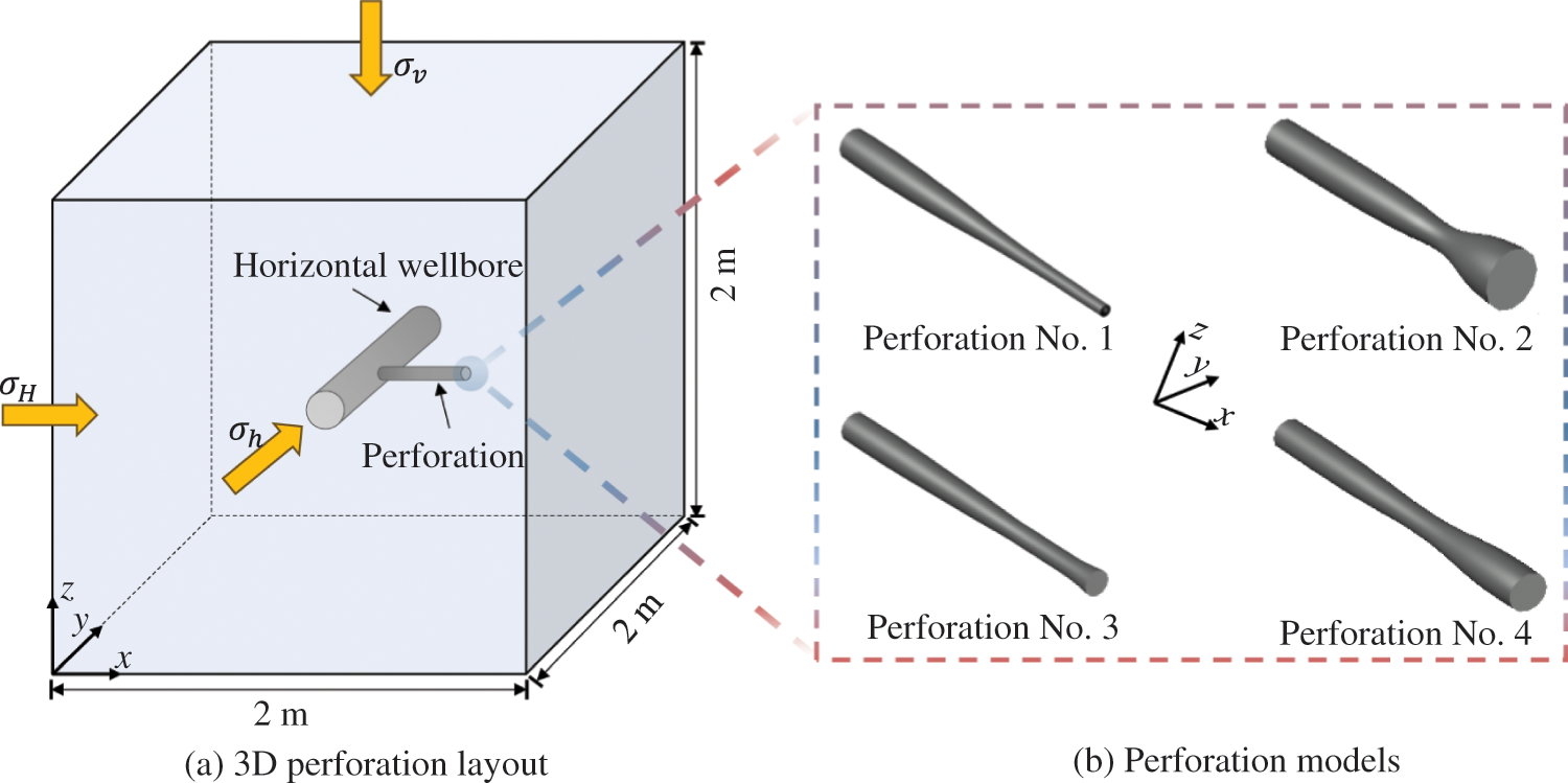
Figure 13: Perforation layout and model establishment

4.3 Parameters Setting

In this study, an ideal homogeneous model is utilized without considering the effect of natural fractures. Porous permeability is not accounted for in the simulation, and constant flow loading is employed to inject water into the fracture joints at the end of perforation. The stress and seepage boundary conditions are applied to the model. Material properties of rock strata and the magnitude of the three-dimensional in-situ stress can be obtained from geological exploration data in the engineering report. The seepage conditions are applied with the same values as in Section 3.3. Based on the geological stress exploration data. Some parameters are calibrated in Table 3, while the remaining parameters are detailed in Table 6.

4.4 Simulation Results

Saturation signifies the extent to which fluid permeates the fracture grid, where a value of 1 denotes complete filling and 0 indicates no fluid flow. Fig. 14 visually illustrates the changes in saturation for the four perforation types. Water pressure is applied around the open-hole perforation wall, and over 1 to 60 s, fluid gradually permeates the surrounding rock formations from the perforation surface. Fig. 14 provides a visual representation of the loading process, indicating the location and shape of the perforations.

Figure 14: Saturation cloud images of four perforations ((a) Perforation No. 1; (b) Perforation No. 2; (c) Perforation No. 3; (d) Perforation No. 4)

Breakdown pressure serves as a crucial indicator of fracturing effectiveness. As illustrated in Fig. 15, the fluid pressure during loading initially increases, then decreases, and eventually stabilizes. The numerical simulation utilizes the cracking of a block element to describe the generation of fluid channels. Owing to the specific volume of the block and the interaction force between the blocks, the pressure curve will not sharply decrease after the fracture. The breakdown pressures for Perforations No. 1 through 4 are 68.02, 64.01, 68.56, and 65.37 MPa, respectively, with Perforation No. 3 exhibiting the highest breakdown pressure and Perforation No. 2 demonstrating the lowest breakdown pressure.

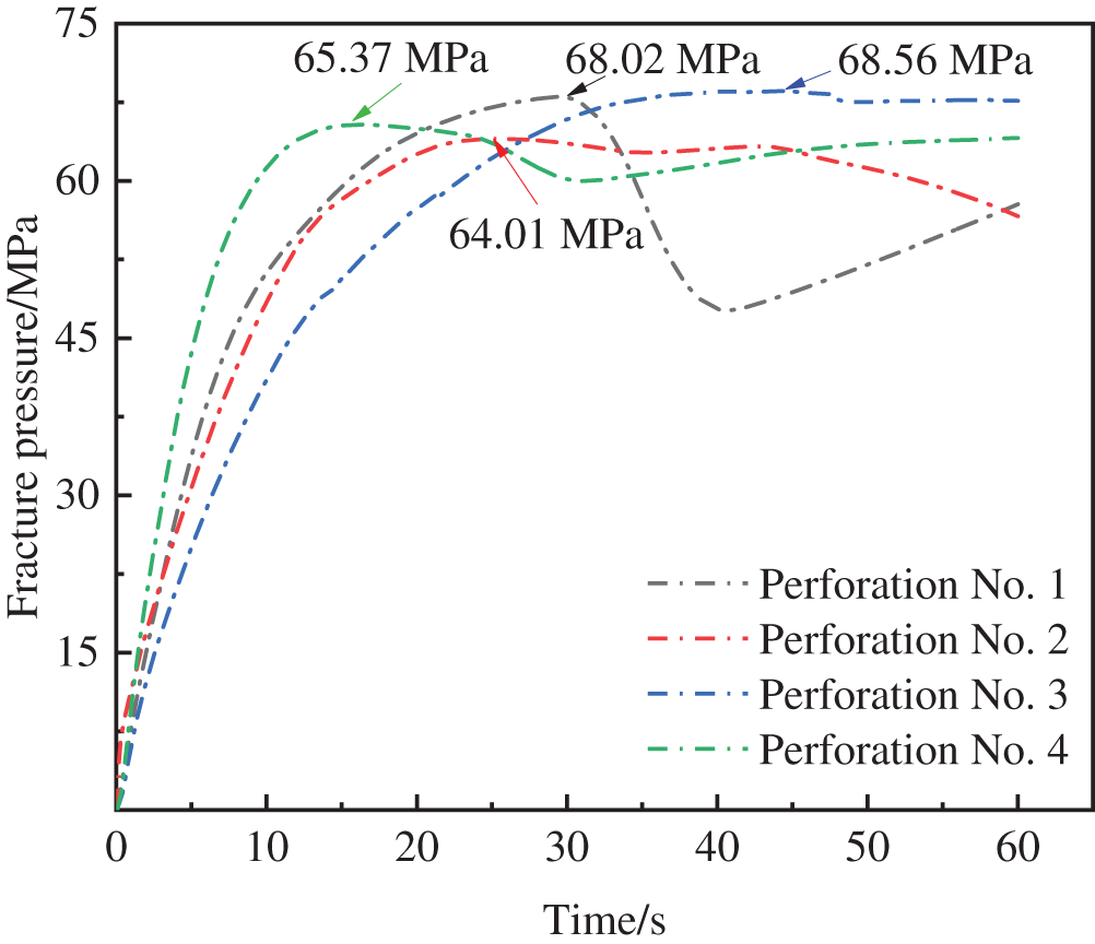
Figure 15: Fracture curves of four perforations

The breakdown pressure determines the difficulty of reservoir cracking, while the fracture network generated by perforation can enhance the reservoir’s permeability. By capturing the dynamic propagation process of hydraulic fractures, the impact of fracturing can be studied. Fig. 16 displays the process of fracture propagation for the four perforations. Initial cracks in the model occurred at 10 s. Due to the drastic change in the interface size of the perforating root, stress concentration and cracks are easily generated, primarily at the junction of the wellbore and perforation during the initial stage. As fracturing progresses, the fracture spreads from the root of the perforation to the middle, forming a complex network around it. By 60 s, the fracture has enveloped the entire perforation channel. Fig. 17 illustrates the failure state of the four perforations, with 0 indicating no damage, 1 indicating tensile damage, and 2 indicating shear damage. Under the influence of fluid pressure, the perforation consistently surpasses the tensile strength of the rock mass, resulting in primarily tensile failure. Fig. 18 shows the stress distribution of the four perforations in x direction. At 10 s, perforation was in the early stage of fracture. At this point, the area with significant tensile stress is at the root of the perforation (the junction of the perforation and the wellbore), where the cross-section undergoes significant changes, making stress concentration likely.

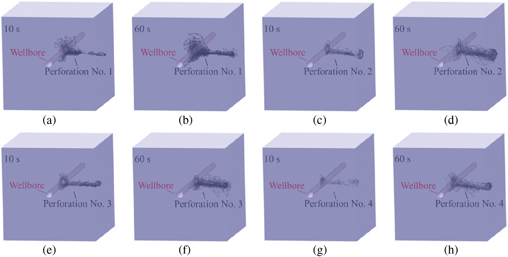
Figure 16: Fracture propagation diagram of four perforations ((a)~(b) Fracture propagation diagram of Perforation No. 1; (c)~(d) Fracture propagation diagram of Perforation No. 2; (e)~(f) Fracture propagation diagram of Perforation No. 3; (g)~(h) Fracture propagation diagram of Perforation No. 4)

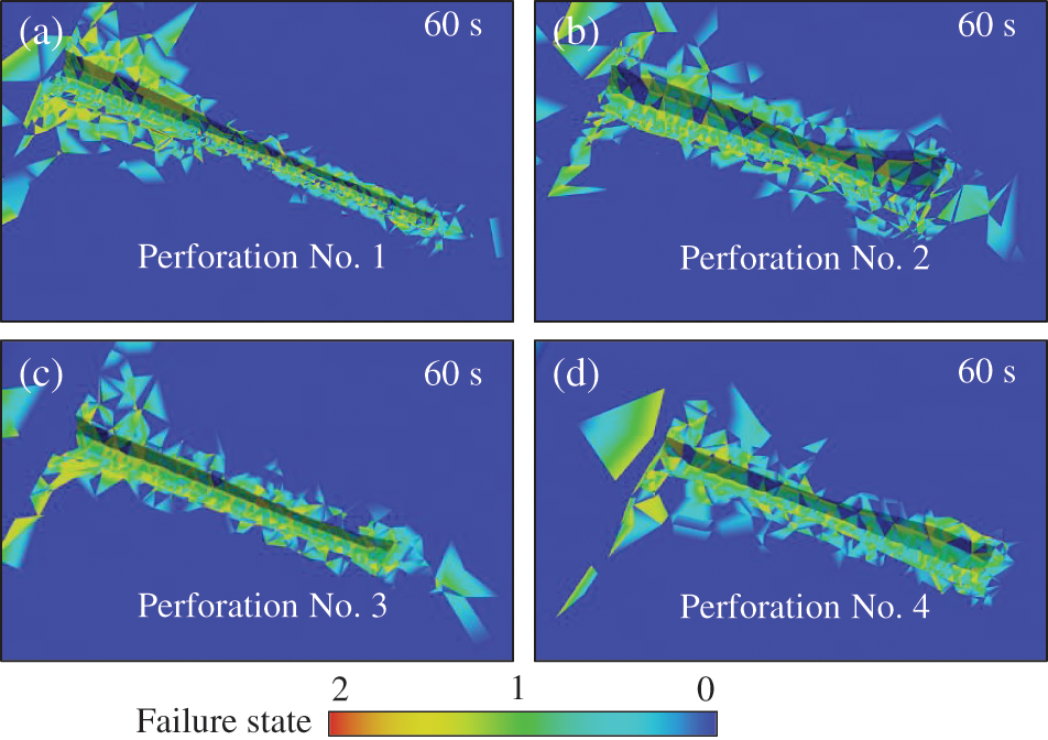
Figure 17: Failure state of four perforations ((a) Perforation No. 1; (b) Perforation No. 2; (c) Perforation No. 3; (d) Perforation No. 4)

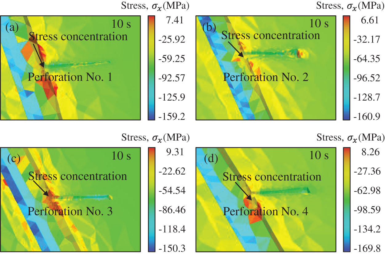
Figure 18: Stress distribution in x direction of four perforations ((a) Perforation No. 1; (b) Perforation No. 2; (c) Perforation No. 3; (d) Perforation No. 4)

The complexity of the fracture network can be quantitatively analyzed by the fracture degree. Fracture degree is defined as the ratio of the area of the contact surface that fractures to the total area of the contact surface that can be fractured [63]. This metric characterizes the complexity of the fracture network in the rock. As depicted in Fig. 19, Perforation No. 3 exhibited the smallest fracture degree, whereas Perforation No. 2 displayed the largest fracture degree. With decreasing the breakdown pressure, the fracture degree of the perforation increases. The relatively large length and section diameter of Perforation No. 2 result in a larger volume, potentially leading to a greater fracture degree due to this initial defect. Ultimately, among the four types of penetrating bullets, the Perforation No. 2 formed by the 39g DP3 HMX perforating bullet exhibited the lowest breakdown pressure and the highest fracture degree.

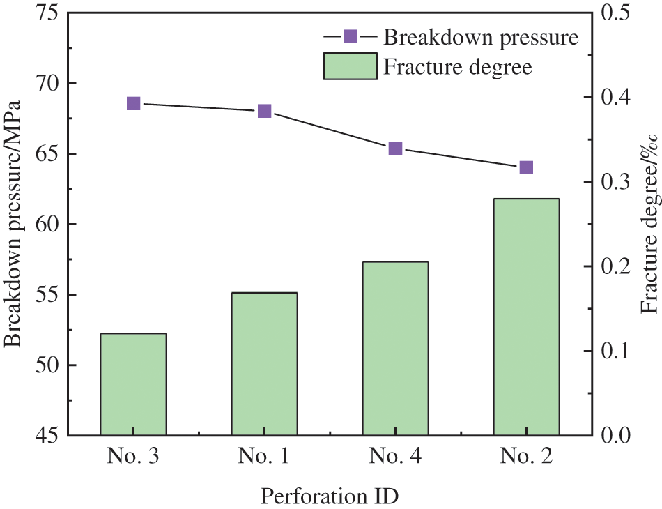
Figure 19: Fracture degree and breakdown pressure of four perforations

5  Influence of Perforation Shape on Hydraulic Fracturing

5.1 Simulation Model Setting

Based on Perforation No. 2, modifications were made to the parameters of the perforation shape to explore their influence on fracturing outcomes, encompassing penetration length and cross-section diameter. To clearly observe the distinct patterns of change, a significant gradient in parameter modification was employed. As depicted in Table 7, “Perforation No. 2” serves as the reference model. Models 1-1, 1-2, and 1-3 compare the variable cross-section column with the equal cross-section cylinder perforation, where the radii of the equal cross-section cylinders 1-1 and 1-2 align with the radii of the ends of Perforation No. 2. Model 1-3 represents a cylindrical perforation of equal section, matching the volume and length of Perforation No. 2, featuring a radius d1−3 of 36.34 mm, as calculated from Eq. (22).

VP2=π(12d1−3)2(lN+lD)(22)

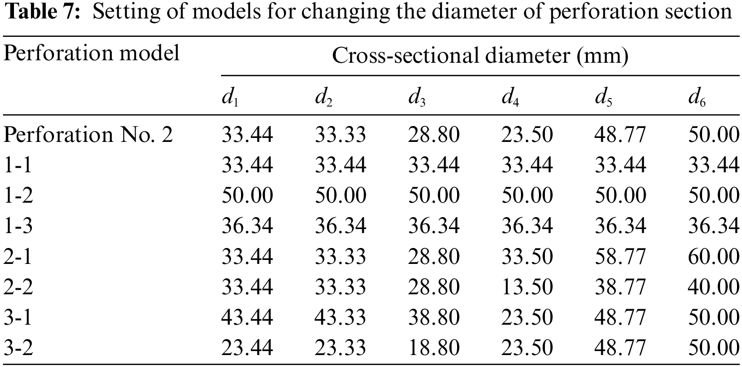
where VP2 represents the volume of Perforation No. 2, which can be calculated by CAD software.

In Models 2-1 and 2-2, the radius of each cross-section in the far-well section was increased (or decreased) by 5 mm, and in Models 3-1 and 3-2, the radius of each near-well section was increased (or decreased) by 5 mm, as detailed in Table 8. Models 4-1 and 4-2 involved changes in the length of Perforation No. 2, with the length of each small section being increased (or decreased) by 10 mm. To visually compare the differences in perforation sizes, Fig. 20 presents the 3D perforation patterns in each model.

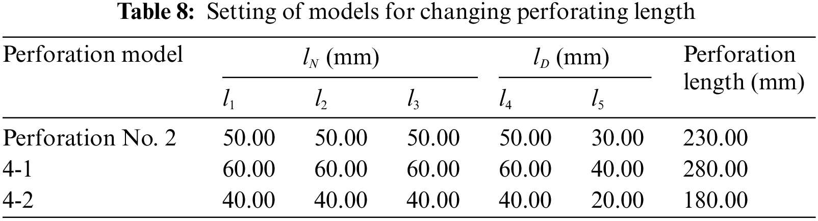
Figure 20: Schematic of the perforation in three dimensions ((a~c) Equal cross-section cylinder; (d~e) Change the diameter of the far-well section; (f~g) Change the diameter of the near-well section; (h~i) Change the perforating length)

5.2 Simulation Results and Analysis

Previous investigations did not specify the method used to simplify the perforation into an equal cross-section cylinder. In Fig. 21a, when the minimum and maximum radius of Perforation No. 2 are used as the radii of equal cross-section cylinders, the breakdown pressures are 66.83 MPa (Model 1-1) and 53.86 MPa (Model 1-2), respectively. The breakdown pressure of Perforation No. 2 falls between these two values, with pressure differences of 2.82 and 10.15 MPa, respectively. With the influence of water pressure, the rock mass primarily overcomes the tensile strength after overcoming the effects of in-situ stress. Comparing the difference of breakdown pressure and tensile strength of different perforations can significantly indicate the difficulty of cracking. The two difference values account for 94.0% and 338.3% of the rock tensile strength (3 MPa), respectively. Under the same volume, the breakdown pressure is 65.35 MPa (Model 1-3), which is 1.34 MPa higher than that of Perforation No. 2 and represents 44.7% of the rock tensile strength (3 MPa). These results suggest that a significant deviation in breakdown pressure may occur when the perforation is simplified into an equal cross-section cylinder.

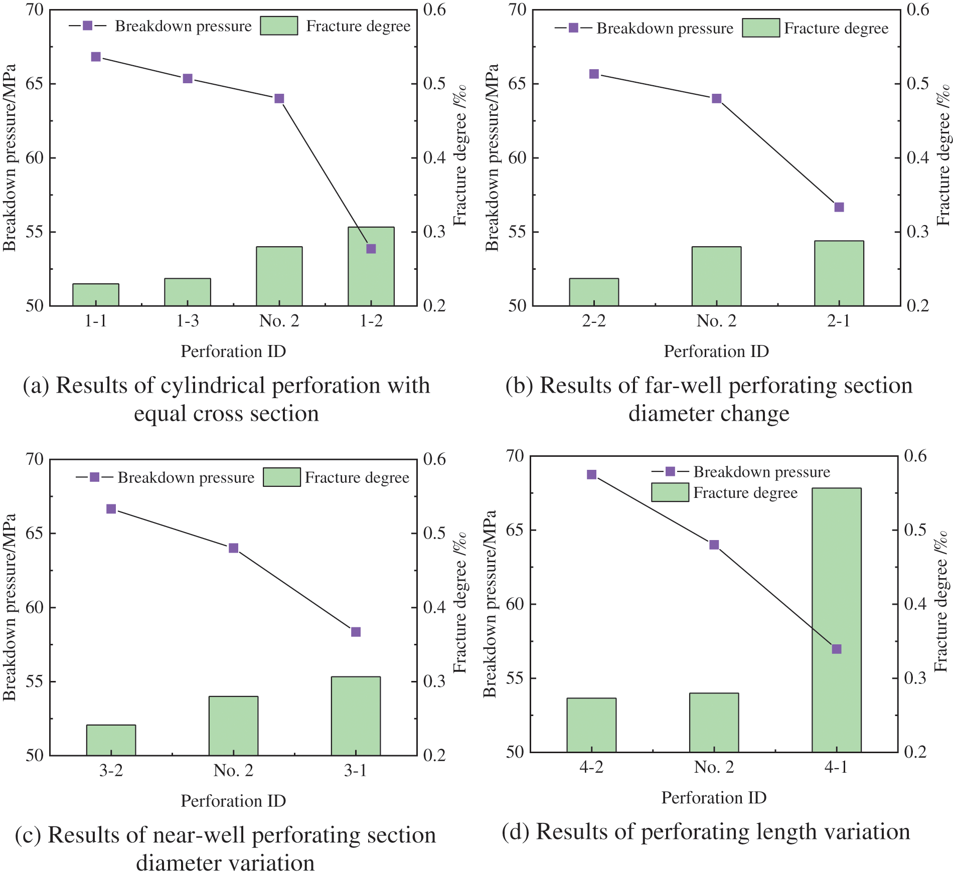
Figure 21: Fracture degree and breakdown pressure of various models

Figs. 21b and 21c illustrate that increasing the cross-section diameter of both the far-well section and near-well section yields breakdown pressures of 56.67 MPa (Model 2-1) and 58.35 MPa (Model 3-1), respectively. Conversely, reducing the perforation cross-section diameter of the far-well section and near-well section leads to breakdown pressures of 65.67 MPa (Model 2-2) and 66.66 MPa (Model 3-2), respectively. Overall, there is a negative correlation between breakdown pressure and perforation diameter, which aligns with findings from research on simplified regular-shaped perforations [23,55]. Increasing the perforation diameter enlarges the size difference around the perforation channel, intensifying the weakening effect on the rock mass and rendering the perforation more susceptible to cracking. Consequently, this results in a decrease in the perforation breakdown pressure.

In Fig. 21d, the breakdown pressures are 68.75 MPa (Model 4-1) and 56.97 MPa (Model 4-2) when the penetration length is increased, respectively. Increasing the penetration length expands the effective area of fluid pressure on the hole wall, resulting in greater fluid energy used to break the rock layer. Consequently, this increases the circumferential stress of the borehole, potentially reducing the breakdown pressure.

Fig. 21 indicates that a decrease in breakdown pressure is associated with an increase in fracture degree when a single parameter is changed. Additionally, when changing the perforation shape, the breakdown pressure and fracture degree of Model 1-2 (large uniform cross-section cylinder, 53.86 MPa, 0.31‰) are lower than those of Model 4-1 (increased perforation length, 56.97 MPa, 0.56‰). This suggests that perforations with irregular sections are more likely to induce crack propagation than those with equal radius sections after perforation initiation.

6  Conclusions

The conclusions of this study can be summarized as follows:

(1)   Perforation geometries demonstrate a pattern of regularity, deviating from ideal cylindrical shapes. These real-world perforations are characterized by an initial constriction followed by an expansion, a trait consistent across the four examined types. The 39g DP3 HMX perforating bullet was found to produce the lowest breakdown pressure and a significant fracture degree. Conversely, the 95-type deep-penetrating perforating bullet resulted in the highest breakdown pressure and the least extent of fracturing.

(2)   Different simplification approaches for the perforation model have distinct impacts on the outcomes. Modeling the perforation as a cylinder with a uniform cross-section can lead to considerable discrepancies in predicted breakdown pressure. Using the diameter of the perforation entry as the basis for the cylinder’s diameter yields a breakdown pressure that diverges from that of a detailed perforation model. Variations in breakdown pressure among cylindrical perforations with equivalent volumes are relatively minor.

(3)   An inverse relationship was identified between breakdown pressure and perforation diameter when variations were restricted to the diameters of the far-well and near-well sections. In a similar vein, breakdown pressure showed a negative correlation with perforation length when adjustments were made solely to the lengths of the far-well and near-well sections. Additionally, an increase in the degree of fracturing corresponded with a decrease in breakdown pressure. Perforations with non-uniform cross-sections were more prone to facilitate crack propagation than those with uniform radii, despite having comparable breakdown pressures.

This research sheds light on the variability of perforation shapes under actual conditions, a notion not previously explored, and provides a numerical approach for optimizing perforation design. It also offers a basis for further investigation into the effects of perforation geometry on fracturing behavior. However, the acquisition of field data remains a challenge, and further experimental validation is necessary to corroborate the findings of this study.

Acknowledgement: The authors acknowledge the assistance of two doctors, Zhiran Gao and Junlin Wang (School of Civil and Transportation Engineering, Hebei University of Technology, China). Dr. Gao provided some necessary textual information to improve the feasibility of the study. Dr. Wang provided guidance and assistance in numerical methods. In addition, the authors thank the anonymous reviewers and journal editors for their constructive comments.

Funding Statement: The authors gratefully acknowledge the financial support from the National Natural Science Foundation of China (Grant Nos. 52178324, 12102059), the China Postdoctoral Science Foundation (Grant No. 2023M743604), the Beijing Natural Science Foundation (Grant No. 3212027), the National Key R&D Program of China (Grant No. 2023YFC3007203), and the 2019 Foreign Experts Plan of Hebei Province.

Author Contributions: The authors confirm their contribution to the paper as follows: Rui Zhang: Software, Writing–original draft. Lixiang Wang: Funding acquisition, Writing–review & editing. Chun Feng: Supervision. Jing Li: Investigation, Conceptualization. Chun Feng and Yiming Zhang: Funding acquisition. All authors reviewed the results and approved the final version of the manuscript.

Availability of Data and Materials: The data that support the findings of this study are available from the corresponding authors on reasonable request.

Conflicts of Interest: The authors declare that they have no conflicts of interest to report regarding the present study.

References

1. Cui Y, Lu C, Wu M, Peng Y, Yao Y, Luo W. Review of exploration and production technology of natural gas hydrate. Adv Geo-Energy Res. 2018;2(1):53–62. doi:10.26804/ager.2018.01.05. [Google Scholar] [CrossRef]

2. Bai Q, Liu Z, Zhang C, Wang F. Geometry nature of hydraulic fracture propagation from oriented perforations and implications for directional hydraulic fracturing. Comput Geotech. 2020;125:103682. doi:10.1016/j.compgeo.2020.103682. [Google Scholar] [CrossRef]

3. Cheng Y, Lu Y, Ge Z, Cheng L, Zheng J, Zhang W. Experimental study on crack propagation control and mechanism analysis of directional hydraulic fracturing. Fuel. 2018;218:316–24. doi:10.1016/j.fuel.2018.01.034. [Google Scholar] [CrossRef]

4. Liu H, Wang F, Wang Y, Gao Y, Cheng J. Oil well perforation technology: Status and prospects. Pet Explor Dev. 2014;41(6):798–804. doi:10.1016/S1876-3804(14)60096-3. [Google Scholar] [CrossRef]

5. Fan Y, Zhu Z, Zhao Y, Zhou C, Zhang X. The effects of some parameters on perforation tip initiation pressures in hydraulic fracturing. J Petrol Sci Eng. 2019;176:1053–60. doi:10.1016/j.petrol.2019.02.028. [Google Scholar] [CrossRef]

6. Chen Z, Qiu J, Chen Q, Li X, Ma B, Huang X. Influence of multi-perforations hydraulic fracturing on stress and fracture characteristics of hard rock mass under excavation condition. Eng Fract Mech. 2022;276:108925. doi:10.1016/j.engfracmech.2022.108925. [Google Scholar] [CrossRef]

7. Qin C, Ma C, Li L, Sun X, Liu Z, Sun Z. Development and application of an intelligent robot for rock mass structure detection: A case study of Letuan tunnel in Shandong China. Int J Rock Mech Min Sci. 2023;169:105419. doi:10.1016/j.ijrmms.2023.105419. [Google Scholar] [CrossRef]

8. Detournay E, Carbonell R. Fracture-mechanics analysis of the breakdown process in minifracture or leakoff test. SPE Prod Facil. 1997;12(3):195–9. doi:10.2118/28076-PA. [Google Scholar] [CrossRef]

9. Zeng Y, Jin X, Ding S, Zhang B, Bian X, Shah S, et al. Breakdown pressure prediction with weight function method and experimental verification. Eng Fract Mech. 2019;214:62–78. doi:10.1016/j.engfracmech.2019.04.016. [Google Scholar] [CrossRef]

10. Chen M, Guo T, Qu Z, Sheng M, Mu L. Numerical investigation into hydraulic fracture initiation and breakdown pressures considering wellbore compliance based on the boundary element method. J Petrol Sci Eng. 2022;211:110162. doi:10.1016/j.petrol.2022.110162. [Google Scholar] [CrossRef]

11. Behrmann LA, Elbel JL. Effect of perforations on fracture initiation. JPT J Pet Technol. 1991;43(5):608–15. doi:10.2118/20661-PA. [Google Scholar] [CrossRef]

12. Abass HH, Meadows DL, Brumley JL, Hedayati S, Venditto JJ. Oriented perforations-a rock mechanics view. In: SPE Annual Technical Conference and Exhibition, 1994 Sep 25–28; New Orleans, Louisiana, USA. doi:10.2118/28555-MS. [Google Scholar] [CrossRef]

13. Zhang R, Hou B, Shan Q, Tan P, Wu Y, Gao J, et al. Hydraulic fracturing initiation and near-wellbore nonplanar propagation from horizontal perforated boreholes in tight formation. J Nat Gas Sci Eng. 2018;55:337–49. doi:10.1016/j.jngse.2018.05.021. [Google Scholar] [CrossRef]

14. Zheng H, Pu C, Wang Y, Sun C. Experimental and numerical investigation on influence of pore-pressure distribution on multi-fractures propagation in tight sandstone. Eng Fract Mech. 2020;230:106993. doi:10.1016/j.engfracmech.2020.106993. [Google Scholar] [CrossRef]

15. Zhai L, Xun Y, Liu H, Qi B, Wu J, Wang Y, et al. Experimental study of hydraulic fracturing initiation and propagation from perforated wellbore in oil shale formation. Fuel. 2023;352:129155. doi:10.1016/j.fuel.2023.129155. [Google Scholar] [CrossRef]

16. Wang LX, Wen LF, Wang JT, Tian R. Implementations of parallel software for crack analyses based on the improved XFEM. Sci Sin Tech. 2018;48(11):1241–58 (In Chinese). doi:10.1360/N092017-00367. [Google Scholar] [CrossRef]

17. Wen LF, Tian R, Wang LX, Feng C. Improved XFEM for multiple crack analysis: Accurate and efficient implementations for stress intensity factors. Comput Methods Appl Mech Eng. 2023;411:116045. doi:10.1016/j.cma.2023.116045. [Google Scholar] [CrossRef]

18. Wang LX, Wen LF, Tian R, Feng C. Improved XFEM (IXFEMArbitrary multiple crack initiation, propagation and interaction analysis. Comput Methods Appl Mech Eng. 2024;421:116791. doi:10.1016/j.cma.2024.116791. [Google Scholar] [CrossRef]

19. Shauer N, Duarte CA. A generalized finite element method for three-dimensional hydraulic fracture propagation: comparison with experiments. Eng Fract Mech. 2020;235:107098. doi:10.1016/j.engfracmech.2020.107098. [Google Scholar] [CrossRef]

20. Cundall PA. A computer model for simulating progressive, large-scale movement in blocky rock system. In: Proceedings of the International Symposium on Rock Mechanics, 1971; Nancy, France. p. 129–36 [Google Scholar]

21. Zhang X, Si G, Bai Q, Xiang Z, Li X, Oh J, et al. Numerical simulation of hydraulic fracturing and associated seismicity in lab-scale coal samples: A new insight into the stress and aperture evolution. Comput Geotech. 2023;160:105507. doi:10.1016/j.compgeo.2023.105507. [Google Scholar] [CrossRef]

22. Ben Y, Xue J, Miao Q, Wang Y, Shi G. Simulating hydraulic fracturing with discontinuous deformation analysis. In: The 46th U.S. Rock Mechanics/Geomechanics Symposium, 2012 Jun 24–27; Chicago, Illinois, USA. [Google Scholar]

23. Zhang H, Chen J, Zhao Z, Qiang J. Hydraulic fracture network propagation in a naturally fractured shale reservoir based on the well factory model. Comput Geotech. 2023;153:105103. doi:10.1016/j.compgeo.2022.105103. [Google Scholar] [CrossRef]

24. Abdollahipour A, Marji MF. A thermo-hydromechanical displacement discontinuity method to model fractures in high-pressure, high-temperature environments. Renew Energy. 2020;153:1488–1503. doi:10.1016/j.renene.2020.02.110. [Google Scholar] [CrossRef]

25. Sun J, Löhnert S. 3D thermo-mechanical dynamic crack propagation with the XFEM and gradient enhanced damage. Proc Appl Math Mech. 2021;20(1):e202000271. doi:10.1002/pamm.202000271. [Google Scholar] [CrossRef]

26. Zhuang X, Zhou S, Huynh GD, Areias P, Rabczuk T. Phase field modeling and computer implementation: A review. Eng Fract Mech. 2022;262:108234. doi:10.1016/j.engfracmech.2022.108234. [Google Scholar] [CrossRef]

27. Zhuang X, Li X, Zhou S. Transverse penny-shaped hydraulic fracture propagation in naturally-layered rocks under stress boundaries: a 3D phase field modeling. Comput Geotech. 2023;155:105205. doi:10.1016/j.compgeo.2022.105205. [Google Scholar] [CrossRef]

28. Zhang Y, Lackner R, Zeiml M, Mang HA. Strong discontinuity embedded approach with standard SOS formulation: element formulation, energy-based crack-tracking strategy, and validations. Comput Methods Appl Mech Eng. 2015;287:335–66. doi:10.1016/j.cma.2015.02.001. [Google Scholar] [CrossRef]

29. Zhang Y, Huang J, Yuan Y, Mang HA. Cracking elements method with a dissipation-based arc-length approach. Finite Elem Anal Des. 2021;195:103573. doi:10.1016/j.finel.2021.103573. [Google Scholar] [CrossRef]

30. Zhang Y, Zhuang X. Cracking elements method for dynamic brittle fracture. Theor Appl Fract Mech. 2019;102:1–9. doi:10.1016/j.tafmec.2018.09.015. [Google Scholar] [CrossRef]

31. Yu H, Chen X, Sun Y. A generalized bond-based peridynamic model for quasi-brittle materials enriched with bond tension-rotation-shear coupling effects. Comput Methods Appl Mech Eng. 2020;372:113405. doi:10.1016/j.cma.2020.113405. [Google Scholar] [CrossRef]

32. Zhou X, Wang Y, Shou Y. Hydromechanical bond-based peridynamic model for pressurized and fluid-driven fracturing processes in fissured porous rocks. Int J Rock Mech Min Sci. 2020;132:104383. doi:10.1016/j.ijrmms.2020.104383. [Google Scholar] [CrossRef]

33. Liu Z, Ma Z, Liu K, Zhao S, Wang Y. Coupled CEL-FDEM modeling of rock failure induced by high-pressure water jet. Eng Fract Mech. 2023;277:108958. doi:10.1016/j.engfracmech.2022.108958. [Google Scholar] [CrossRef]

34. Cui W, Liu Q, Wu Z, Xu X. Fracture development around wellbore excavation: Insights from a 2D thermo-mechanical FDEM analysis. Eng Fract Mech. 2024;295:109774. doi:10.1016/j.engfracmech.2023.109774. [Google Scholar] [CrossRef]

35. Zhou X, Bi J, Qian Q. Numerical simulation of crack growth and coalescence in rock-like materials containing multiple pre-existing flaws. Rock Mech Rock Eng. 2015;48:1097–1114. doi:10.1007/s00603-014-0627-4. [Google Scholar] [CrossRef]

36. Wang L, Zhou X. A field-enriched finite element method for simulating the failure process of rocks with different defects. Comput Struct. 2021;250:106539. doi:10.1016/j.compstruc.2021.106539. [Google Scholar] [CrossRef]

37. Wang LX, Li SH, Zhang GX, Ma ZS, Zhang L. A GPU-based parallel procedure for nonlinear analysis of complex structures using a coupled FEM/DEM approach. Math Prob Eng. 2013;2013:618980. doi:10.1155/2013/618980. [Google Scholar] [CrossRef]

38. Feng C, Li SH, Liu XY, Zhang YN. A semi-spring and semi-edge combined contact model in CDEM and its application to analysis of Jiweishan landslide. J Rock Mech Geotech Eng. 2014;6(1):26–35. doi:10.1016/j.jrmge.2013.12.001. [Google Scholar] [CrossRef]

39. Wang LX, Tang DH, Li SH, Wang J, Feng C. Numerical simulation of hydraulic fracturing by a mixed method in two dimensions. Chin J Theor Appl Mech. 2015;47(6):973–83 (In Chinese). doi:10.6052/0459-1879-15-097. [Google Scholar] [CrossRef]

40. Li SH, Feng C, Zhou D. Mechanical methods in landslide research. Beijing, China: Science Press; 2018 (In Chinese). [Google Scholar]

41. Nie W, Wang J, Feng C, Zhang Y. Continuous-discontinuous element method for three-dimensional thermal cracking of rocks. J Rock Mech Geotech Eng. 2023;15(11):2917–29. doi:10.1016/j.jrmge.2023.02.017. [Google Scholar] [CrossRef]

42. Zhu XG, Feng C, Cheng PD, Wang XQ, Li SH. A novel three-dimensional hydraulic fracturing model based on continuum-discontinuum element method. Comput Methods Appl Mech Eng. 2021;383:113887. doi:10.1016/j.cma.2021.113887. [Google Scholar] [CrossRef]

43. Wang LX, Li SH, Feng C. Lagrange’s equations for seepage flow in porous media with a mixed Lagrangian-Eulerian description. Acta Mech Sin. 2023;39(11):323022. doi:10.1007/s10409-023-23022-x. [Google Scholar] [CrossRef]

44. Li J, Wang LX, Feng C, Zhang R, Zhu XG, Zhang YM. Study on the influence of perforation parameters on hydraulic fracture initiation and propagation based on CDEM. Comput Geotech. 2024;167:106061. doi:10.1016/j.compgeo.2023.106061. [Google Scholar] [CrossRef]

45. Han W, Cui Z, Zhang J. Fracture path interaction of two adjacent perforations subjected to different injection rate increments. Comput Geotech. 2020;122:103500. doi:10.1016/j.compgeo.2020.103500. [Google Scholar] [CrossRef]

46. Cheng S, Wu B, Zhang M, Zhang X, Han Y, Jeffrey RG, et al. Surrogate modeling and global sensitivity analysis for the simultaneous growth of multiple hydraulic fractures. Comput Geotech. 2023;162:105709. doi:10.1016/j.compgeo.2023.105709. [Google Scholar] [CrossRef]

47. Zhang H, Chen J, Gong D, Liu H, Ouyang W. Effects of fracturing parameters on fracture network evolution during multicluster fracturing in a heterogeneous reservoir. Comput Geotech. 2023;159:105474. doi:10.1016/j.compgeo.2023.105474. [Google Scholar] [CrossRef]

48. Sepehri J, Soliman MY, Morse SM. Application of extended finite element method (XFEM) to simulate hydraulic fracture propagation from oriented perforations. In: The SPE Hydraulic Fracturing Technology Conference, 2015 Feb 3–5; Texas, USA. doi:10.2118/SPE-173342-MS. [Google Scholar] [CrossRef]

49. Song C, Chen Y, Wang J. Experiment and simulation for controlling propagation direction of hydrofracture by multi-boreholes hydraulic fracturing. Comput Model Eng Sci. 2019;120(3):779–97. doi:10.32604/cmes.2019.07000. [Google Scholar] [CrossRef]

50. Wang Q, Hu Y, Zhao J, Chen S, Fu C, Zhao C. Numerical simulation of fracture initiation, propagation and fracture complexity in the presence of multiple perforations. J Nat Gas Sci Eng. 2020;83:103486. doi:10.1016/j.jngse.2020.103486. [Google Scholar] [CrossRef]

51. Shi F, Wang D, Chen X. A numerical study on the propagation mechanisms of hydraulic fractures in fracture-cavity carbonate reservoirs. Comput Model Eng Sci. 2021;127(2):575–98. doi:10.32604/cmes.2021.015384. [Google Scholar] [CrossRef]

52. Lu W, He C. Numerical simulation on the initiation and propagation of synchronous perforating fractures in horizontal well clusters. Eng Fract Mech. 2022;266:108412. doi:10.1016/j.engfracmech.2022.108412. [Google Scholar] [CrossRef]

53. Zhao X, Ju Y, Yang Y, Su S, Gong W. Impact of hydraulic perforation on fracture initiation and propagation in shale rocks. Sci China-Tech. 2016;59:756–62. doi:10.1007/s11431-016-6038-x. [Google Scholar] [CrossRef]

54. Shan Q, Zhang R, Jiang Y. Complexity and tortuosity hydraulic fracture morphology due to near-wellbore nonplanar propagation from perforated horizontal wells. J Nat Gas Sci Eng. 2021;89:103884. doi:10.1016/j.jngse.2021.103884. [Google Scholar] [CrossRef]

55. Wanniarachchi WAM, Ranjith PG, Li J, Perera MSA. Numerical simulation of foam-based hydraulic fracturing to optimise perforation spacing and to investigate effect of dip angle on hydraulic fracturing. J Petrol Sci Eng. 2019;172:83–96. doi:10.1016/j.petrol.2018.09.032. [Google Scholar] [CrossRef]

56. Dong K, Li Q, Liu W, Zhao X, Zhang S. Optimization of perforation parameters for horizontal wells in shale reservoir. Energy Rep. 2021;7(S7):1121–30. doi:10.1016/j.egyr.2021.09.157. [Google Scholar] [CrossRef]

57. Huang L, Tan J, Fu H, Liu J, Chen X, Liao X, et al. The non-plane initiation and propagation mechanism of multiple hydraulic fractures in tight reservoirs considering stress shadow effects. Eng Fract Mech. 2023;292:109570. doi:10.1016/j.engfracmech.2023.109570. [Google Scholar] [CrossRef]

58. Bangi MSF, Kwon JSI. Deep hybrid modeling of chemical process: Application to hydraulic fracturing. Comput Chem Eng. 2020;134:106696. doi:10.1016/j.compchemeng.2019.106696. [Google Scholar] [CrossRef]

59. Siddhamshetty P, Yang S, Kwon JSI. Modeling of hydraulic fracturing and designing of online pumping schedules to achieve uniform proppant concentration in conventional oil reservoirs. Comput Chem Eng. 2018;114:306–17. doi:10.1016/j.compchemeng.2017.10.032. [Google Scholar] [CrossRef]

60. Sneddon IN, Lowengrub M. Crack problems in the classical theory of elasticity. New York: Wiley; 1969. doi:10.1137/1013045. [Google Scholar] [CrossRef]

61. Jiang H, Chen M, Zhang G, Jin Y, Zhao Z, Zhu G. Impact of oriented perforation on hydraulic fracture initiation and propagation. Chin J Rock Mech Eng. 2009;28(7):1321–6 (In Chinese). [Google Scholar]

62. Sun F, Xue S, Tang M, Zhang X, Ma B. Impact of in-plane perforations on near-wellbore fracture geometry in horizontal wells. In: The ARMA-CUPB Geothermal International Conference, 2019 Aug 5–8; Beijing, China. [Google Scholar]

63. Guo RK, Feng C, Zhou D, Li SH. Study on the evaluation method of slope disaster status based on the reliability of fracture degree. Chin J Rock Mech Eng. 2016;35(S1):3111–8 (In Chinese). doi:10.13722/j.cnki.jrme.2015.0216. [Google Scholar] [CrossRef]