A Review of Computational Fluid Dynamics Techniques and Methodologies in Vertical Axis Wind Turbine Development

1  Introduction

1.1 Background on Vertical Axis Wind Turbines

Vertical axis wind turbines (VAWTs) offer a compelling alternative to the dominant horizontal axis wind turbines (HAWTs), especially in urban environments where wind conditions are highly turbulent and unpredictable. Unlike HAWTs, which require constant reorientation to face the wind, VAWTs operate efficiently regardless of wind direction, eliminating the need for complex yaw mechanisms and reducing mechanical wear. Their design thrives in the chaotic airflow of cities, where HAWTs often underperform, and their compact, visually distinct form fits better within dense urban settings. Though typically less efficient at converting wind energy, VAWTs trade raw performance for adaptability, lower noise, aesthetic compatibility, and simpler integration into existing infrastructure [1–3]. Additionally, VAWTs can be designed with visually appealing shapes, such as helical or spiral blades, allowing them to blend into architectural designs rather than standing out as industrial intrusions. And therefore, unlike HAWTs, which require tall towers and large rotor diameters, VAWTs can be incorporated into streetlights [4–6] installed on rooftops, along highways, or even integrated into building facades [7–11] (examples are as shown in Fig. 1).

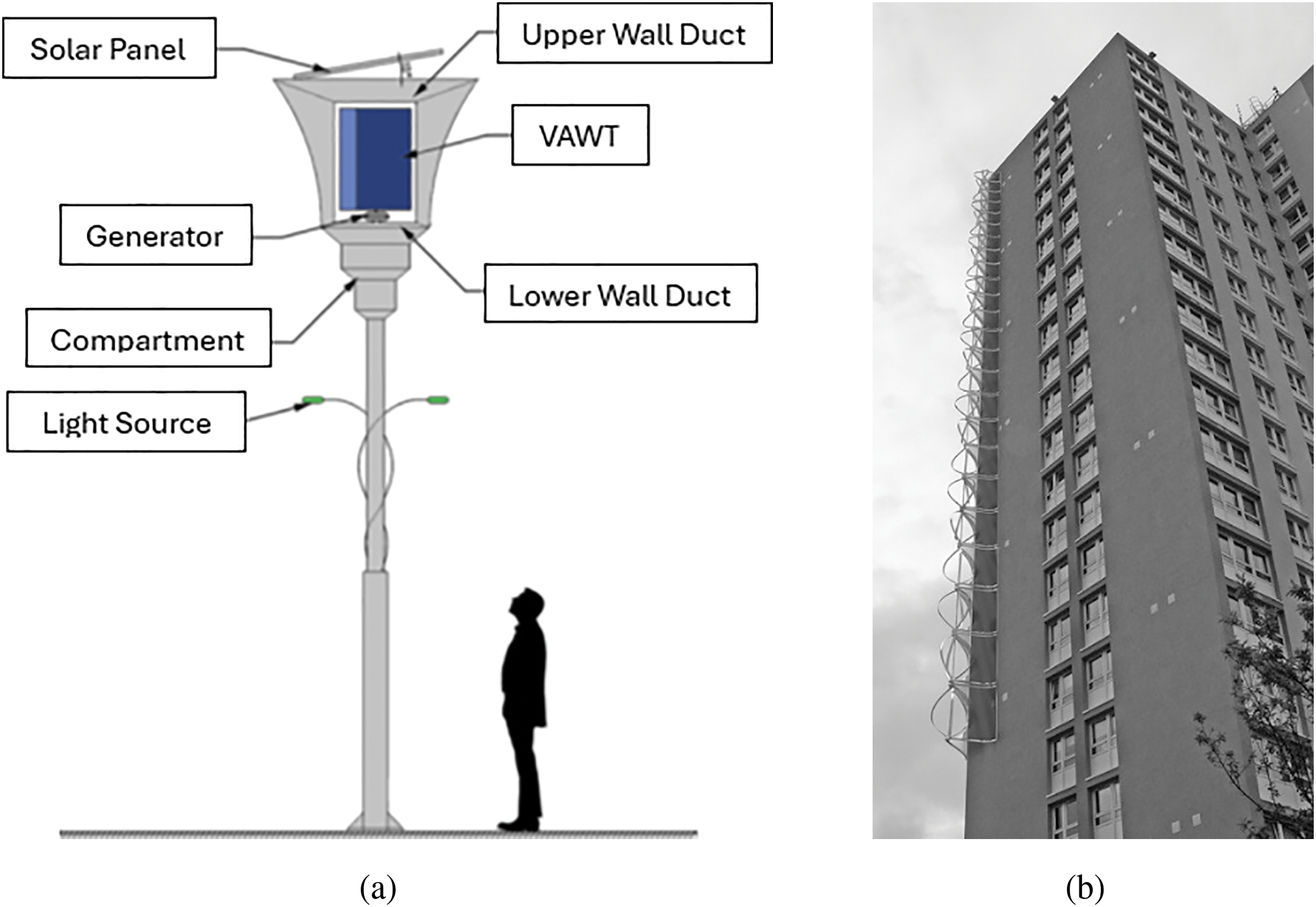
Figure 1: (a) Eco-Greenergy™ hybrid wind-solar energy generation system design and general arrangement [6], (b) Crossflex wind turbine blended into a corner of a building [11]

VAWTs are omnidirectional, meaning they can capture wind from any direction without needing complex yaw systems, making them well-suited for the changing wind conditions in urban areas [7,12,13]. Recent CFD-based works have demonstrated the urban viability of VAWTs. Yu et al. (2025) analyzed gusty inflow effects typical of street-level environments using transient CFD [14]. Saleh et al. (2025) employed ANSYS Fluent to assess helical and IceWind turbines mounted on residential buildings, quantifying both aerodynamic and energy-saving benefits [15]. Their vertical orientation means they occupy less space while still harnessing wind energy effectively. Maintenance becomes easier and safer because their generators and gearboxes are typically located at ground level, which is an essential consideration in densely populated urban areas. Furthermore, VAWTs can operate at lower wind speeds, making them viable even in areas where conventional turbines would be ineffective. Recent advancements in design, such as helical and hybrid models, have improved their efficiency by up to 30% in such environments [12,16]. In other studies, VAWTs arranged in clusters have been shown to have enhanced power output, a promising development that underscores their potential in urban settings [17]. This configuration allows for efficient operation even in turbulent wind conditions typical in urban areas.

Despite their advantages, VAWTs face challenges such as optimising start-up performance and reducing production costs. The future of vertical axis wind turbines (VAWTs) hinges on advancing computational fluid dynamics (CFD) to optimise rotor design, mitigate aerodynamic inefficiencies like dynamic stall, and enhance performance in turbulent urban flows. CFD plays a crucial role in VAWT development by enabling precise simulation of complex blade-wind interactions, allowing for innovations such as helical blades and flow control devices to reduce torque fluctuations and noise [18,19]. However, challenges persist in scaling CFD models from 2-D to 3-D analyses to capture real-world effects like blade tip vortices and structural fatigue, requiring high-fidelity simulations and validation against experimental data [20,21]. While AI-assisted design and hybrid configurations show promise for efficiency gains, standardised methodologies and cost-effective computational frameworks remain critical to overcoming VAWTs’ lower efficiency and durability concerns, particularly in large-scale applications [18,19].

1.2 Fundamentals of Computational Fluid Dynamics

Computational Fluid Dynamics (CFD) is a branch of fluid mechanics that uses numerical methods and computational algorithms to simulate and predict fluid flow behaviour, including properties such as velocity, pressure, temperature, density, and viscosity under defined conditions [22] Acting as a virtual laboratory, CFD allows researchers and engineers to mathematically model fluid dynamics by solving complex governing equations, often replacing or complementing physical experiments [22]. It is widely applied across industries such as aerospace, automotive, energy, environmental, and biomedical engineering—for example, predicting aircraft aerodynamics to reduce wind tunnel testing or improving electric vehicle cooling systems [23]. The foundation of CFD lies in the conservation laws of physics, mathematically expressed through partial differential equations like the Navier-Stokes equations [24], which are typically too complex and non-linear to solve analytically for real-world problems. This complexity necessitates the use of numerical approximation techniques and substantial computing power to generate practical solutions [25,26].

The cornerstone of CFD simulations lies in the mathematical representation of fundamental physical principles governing fluid motion. These principles, universally applied, ensure the conservation of mass, momentum, and energy within a fluid system [24]. The conservation of mass (continuity equation) dictates that the mass within a defined fluid volume must remain constant over time unless there is a net flow of mass across the volume’s boundaries. Mathematically, it relates the rate of change of fluid density (ρ) over time (t) to the divergence of the mass flux [27]. For incompressible flows, where density is assumed constant, this equation simplifies significantly, often relating the divergence of the velocity field to zero. The conservation of momentum, based on Newton’s Second Law, relates the change in momentum of a fluid to forces acting on it, such as pressure, viscosity, and gravity—and is mathematically expressed through the Navier-Stokes equations [27]. They are a set of coupled, non-linear partial differential equations describing the relationship between fluid acceleration, pressure gradients, viscous stresses (often related to velocity gradients via viscosity, μ), and external body forces (fb). Lastly, the conservation of energy (First Law of Thermodynamics) accounts for the transfer and conversion of energy within the fluid system, including heat transfer (conduction, convection, radiation) and work done by or on the fluid [27]: This principle accounts for the transfer and conversion of energy within the fluid system, including heat transfer (conduction, convection, radiation) and work done by or on the fluid. The energy equation is often solved simultaneously with the mass and momentum equations, particularly when temperature variations or heat transfer effects are significant, allowing for the determination of the temperature field alongside velocity and pressure [26]. These governing equations form a closed system when supplemented by appropriate equations of state that relate to thermodynamic properties like pressure, density, and temperature [25].

The development of CFD has closely followed the progress of high-performance computing (HPC). Early CFD work in the mid-20th century relied on simplified equations, but digital computing enabled basic simulations using methods from pioneers like Richardson and Harlow [28–32]. As computer power grew, more advanced techniques and commercial CFD software emerged. Despite these advances, CFD remains computationally intensive, particularly for the complex, three-dimensional turbulent flows that characterize VAWTs [33]. Future advancements, such as widespread use of Direct Numerical Simulation (DNS), will continue to rely on HPC progress [34]. It is crucial to recognise that CFD is fundamentally a modelling process where each step introduces assumptions and potential errors [25,35]. The results are approximations of reality, necessitating a rigorous process of verification and validation against experimental data to build confidence and understand their limitations. As shown in Fig. 2, the practical application of CFD systematically translates a physical fluid problem into a solvable numerical framework through six key stages: problem definition, meshing, equation discretisation, boundary condition application, numerical solution, and post-processing [25].

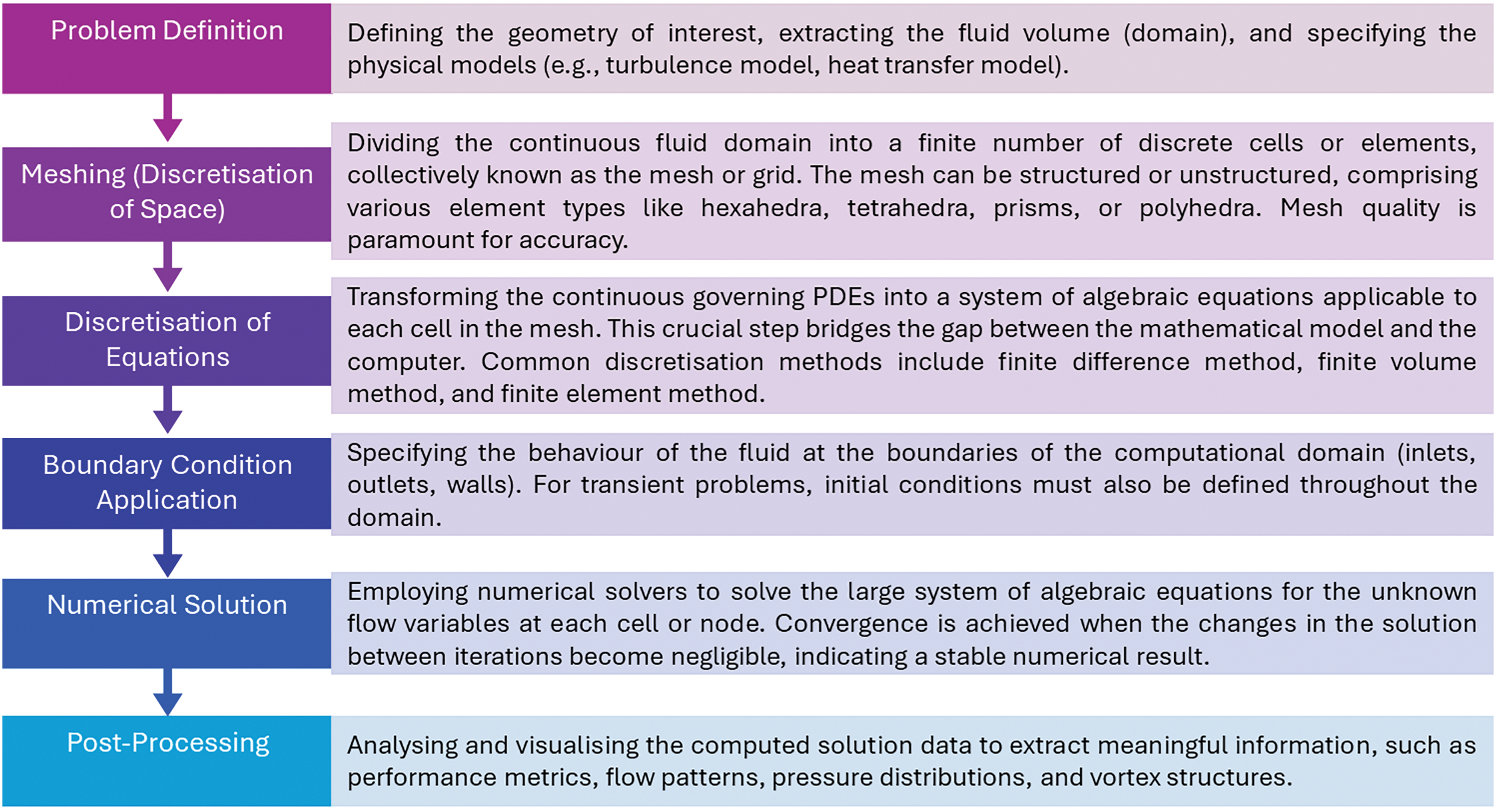
Figure 2: A typical numerical framework consists of problem definition, meshing, discretisation of equations, boundary condition application, numerical solution and finally post-processing

1.3 Contribution of the Current Review

The current review aims to map the evolution and current state of CFD analysis in the context of vertical axis wind turbines, which involves a critical comparison of the different computational approaches applied to VAWT analysis to synthesise insights from the review to highlight areas that may or may not require further exploration. Therefore, the review’s objectives are to identify key studies and trends in CFD analysis of VAWTs, and to analyse the effectiveness of various CFD models and methods.

•   To identify key studies and trends in CFD analysis of VAWTs.

•   To analyse the effectiveness of various CFD models and methods.

•   To identify gaps and future research directions.

2  Vertical Axis Wind Turbines: Designs and Aerodynamic Complexities

Vertical axis wind turbines are characterised by their main rotor shaft being oriented vertically, perpendicular to the ground [36,37]. This fundamental design distinguishes them from the more common Horizontal Axis Wind Turbines (HAWTs) and endows them with inherent advantages.

2.1 Common VAWT Designs

Although the efficiency of horizontal axis turbines is better than that of vertical axis turbines in wind power extraction (as shown in Fig. 3), there are still a lot of significant benefits in deploying vertical axis wind turbines as part of a renewable energy generation strategy [38]. A primary benefit of the vertical axis wind turbine (VAWT) configuration is its omnidirectional capability, allowing it to capture wind from any direction without requiring complex yaw mechanisms to align the rotor with the wind [39,40]. This simplifies the design and control systems, making VAWTs particularly suitable for environments with variable wind directions, such as urban areas or offshore locations [41–44]. Other advantages include placing heavy components at ground level, like the generator and gearbox, facilitating easier installation and maintenance [36]. Additionally, VAWTs are often perceived as producing lower noise emissions because they typically operate at lower tip speeds compared to horizontal axis wind turbines (HAWTs) of similar size, and they may have a reduced visual impact [45]. Furthermore, studies suggest that VAWTs can allow for denser arrangements in wind farms due to faster wake recovery than HAWTs, potentially resulting in higher power output per unit of land area [39]. For detailed information on different VAWT installations and configurations, readers may refer to other excellent reviews, such as the works by [46,47].

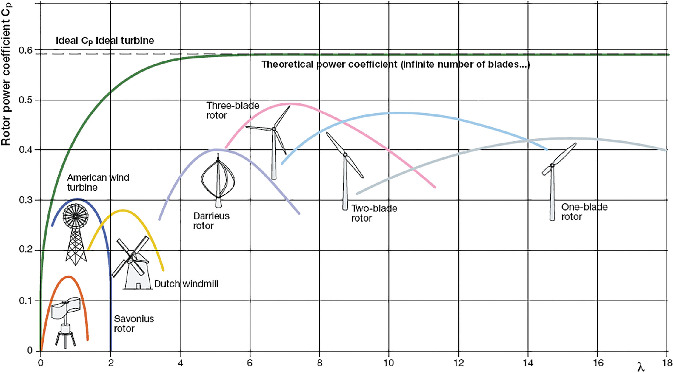
Figure 3: Various wind turbine types and their general power coefficient vs. tip speed ratio characteristic curves [38]

VAWT designs (some examples are shown in Fig. 4) are broadly categorised based on the primary aerodynamic principle they employ [48]:

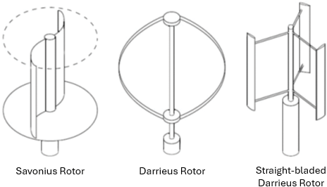
Figure 4: From left to right—Savonius rotor, Darrieus rotor, H-rotor Darrieus (images from [48])

•   Lift-Based (Darrieus Type): Named after Georges Darrieus, these turbines utilise airfoil-shaped blades designed to generate aerodynamic lift as the primary driving force for rotation [42]. The lift force acts predominantly perpendicular to the relative airflow experienced by the blade. Common Darrieus configurations include the original “egg-beater” design with curved blades attached at the top and bottom of the shaft, and the H-rotor (or H-Darrieus) design featuring straight, vertical blades attached to the central shaft via support arms or struts [36,41]. Darrieus turbines can achieve relatively high aerodynamic efficiencies. While large-scale HAWTs can exceed power coefficient, Cp values of 0.45, well-designed research VAWTs typically achieve maximum power coefficients in the 0.35 to 0.42 range [47]. CFD analysis is critical for the blade and rotor optimisation required to reach these higher efficiencies. However, a significant drawback is their typically poor self-starting capability; they often require an external impulse or operate at very low torque at low wind speeds, making it difficult for them to begin rotating from a standstill without assistance [36]. Nonetheless, over the years, research into VAWT has produced a particular novel design based on the Darrieus concept called the cross-axis wind turbine that has improved on the self-starting capabilities of the VAWT [2,49]. Another novel design utilising a vented airfoil based on the NACA0012 profile has been developed to improve torque generation at low tip-speed ratios (TSRs or λ), enhancing self-starting capabilities without significantly affecting performance at high TSRs [50]. Varying the solidity of the Darrieus-type VAWT has also been shown to enhance self-starting. By adjusting solidity, the turbine can self-start in under 30 s at wind speeds of 7.9 m/s, with improved power generation efficiency [51].

•   Drag-Based (Savonius Type): Invented by Sigurd Savonius, these turbines primarily rely on aerodynamic drag forces to generate torque [45]. They typically consist of two or more curved, scoop-like vanes (often resembling an “S” shape in cross-section) [43]. The difference in drag experienced by the advancing (concave) side vs. the returning (convex) side creates a net rotational torque [41]. Savonius turbines are known for their simplicity, robustness, and excellent self-starting characteristics, even at low wind speeds [40]. Their main limitation is significantly lower aerodynamic efficiency compared to Darrieus or HAWT designs [39], where the returning blade generates a counter-acting drag force, limiting the maximum achievable TSR to around unity (λ ≤ 1) and thus capping the potential power extraction [41].

•   Hybrid Designs: Attempts have been made to combine the strengths of both types, most commonly by integrating a Savonius rotor within a Darrieus rotor [40]. The Savonius component intends to provide the necessary starting torque at low speeds, while the Darrieus component delivers higher efficiency at operational speeds. However, the aerodynamic interactions between the two rotor types are complex. The wake shed by the inner Savonius rotor can negatively impact the performance of the outer Darrieus blades, potentially leading to transient load fluctuations and a lower overall peak efficiency compared to an equivalent standalone Darrieus turbine [52].

2.2 Inherent Aerodynamic Challenges of VAWTs

The operation of VAWTs, particularly the lift-driven Darrieus type, involves highly complex and inherently unsteady aerodynamic phenomena [39,42,53]. As a blade traverses its circular path (i.e., the azimuthal angle), the interaction between the freestream wind velocity (U∞ or V) and the blade’s rotational velocity (ωR) causes both the angle of attack (AoA or α)—the angle between the blade chord line and the incoming relative wind—and the magnitude of the relative wind velocity (UT or Vrel) continuously vary throughout each revolution [39,54]. Fig. 5 illustrates this principle. The turbine’s rotation is typically analysed by dividing it into an upwind region (where the blade moves against the incoming wind) and a downwind region (where the blade moves with the wind), as shown in Fig. 5a. As indicated by the velocity triangles in Fig. 5c,d, the changing vector sum of V and ωR, lead to significant variations in α, which in turn influence the lift (or drag) coefficient in the blades (as shown in Fig. 5b). This cyclic variation is the root cause of several significant aerodynamic challenges that complicate analysis and can limit performance.

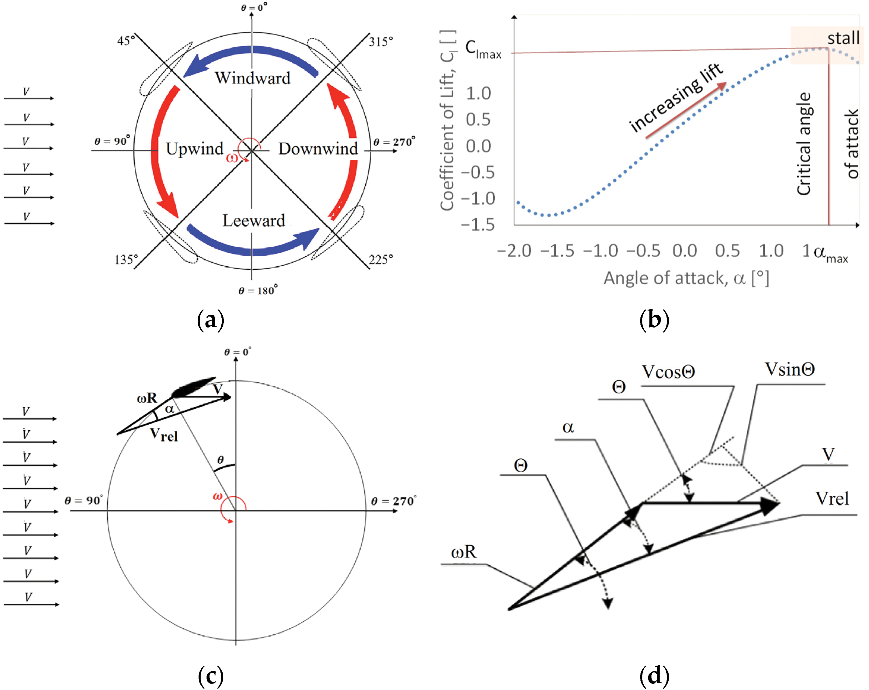
Figure 5: Schematic representation of a vertical axis wind turbine: (a) segmentation of a wind turbine path, (b) lift coefficient, Cl vs. α of an airfoil top surface, (c) schematic 2-D cross section of a single blade as an example of a VAWT blade path, (d) velocity vectors and angles. Adopted from [55]

•   Dynamic Stall: This is arguably the most critical aerodynamic challenge for VAWTs, especially when operating at low Tip Speed Ratios (TSRs), typically below λ ≈ 4 or 5 [39]. Dynamic stall occurs when the blade experiences a rapid change in AoA that significantly exceeds the angle at which stall occurs under steady (static) conditions [42]. Under these dynamic conditions, flow separation is delayed, allowing lift to increase beyond the static maximum for a short period [56]. However, this is followed by the abrupt formation and shedding of large-scale, energetic vortices, primarily the Dynamic Stall Vortex (DSV), often originating near the leading edge [39,42,57,58]. The shedding of the DSV causes an abrupt loss of lift and a sharp increase in drag. This event is directly responsible for the significant torque ripple observed in VAWTs, where the instantaneous torque can fluctuate by over 100% of the mean torque throughout a single revolution [59]. These fluctuations not only reduce the average power output but also induce damaging fatigue loads on the drivetrain and support structure, which can be 2 to 4 times greater than the mean aerodynamic loads [41]. As a result, the overall efficiency and reliability of the turbine are compromised, highlighting the importance of accurate stall prediction and control for advancing VAWT performance [39].

•   Blade-Wake Interactions: As VAWT blades rotate, they inevitably pass through the turbulent wakes generated by the preceding blades and interact with their wake shed during the previous revolution [41,42,60]. This interaction occurs primarily in the downstream half of the rotor’s rotation (leeward side). The blades encounter lower velocity, higher turbulence, and potentially structured vortices within these wakes [58]. This complex interaction further modifies the instantaneous AoA and relative velocity experienced by the blades, impacting their aerodynamic loads and contributing to torque fluctuations and reduced energy extraction in the downstream pass [61]. Current turbulence models used in simulations often struggle to accurately predict the wake characteristics of VAWTs, which can lead to suboptimal design and placement of turbines. Improvements in these models are necessary to better understand and mitigate the effects of blade-wake interactions on efficiency [62]. However, advanced simulation methods have been developed to better capture complex vortex dynamics and wake interactions, which more accurate predictions of wake behaviour and its impact on turbine efficiency [63]

•   Other Complexities: Additional factors contribute to the complex aerodynamics, including the curvature of the flow path experienced by the blades [42], the generation of tip vortices at the blade ends in three-dimensional flows (which influence loads and wake development) [19,64], the effects of operating in skewed or highly turbulent inflow conditions, often found in urban or offshore environments [65], and potentially significant Reynolds number effects, especially for smaller turbines or specific parts of the blade operating at lower relative speeds [66].

Historically, the aerodynamic complexities associated with VAWTs, particularly dynamic stall and wake interactions, have presented significant barriers to their analysis using simpler theoretical models and contributed to their slower commercial development than HAWTs [53,67]. While VAWTs possess attractive characteristics for specific applications, realising their potential hinges on overcoming these aerodynamic challenges. This requires sophisticated analysis tools to capture the unsteady, separated, and vortical flow features inherent to their operation. Advanced computational methods like CFD and targeted experimental validation provide the necessary capabilities to unravel these complexities and guide the development of more efficient and robust VAWT designs [68].

3  An Overview of Setting up CFD Simulations for VAWT Analysis

Conducting meaningful CFD analysis of VAWTs requires careful consideration of the simulation setup, including the computational domain, boundary conditions, mesh generation strategy, turbulence modelling, and solver configuration. These choices significantly impact the simulation’s accuracy, stability, and computational cost.

3.1 Significance of 2-D vs. 3-D Modelling in VAWT CFD Simulations and Analysis

Simulation dimensionality is critical when evaluating turbulence model performance in VAWT CFD applications. Two-dimensional (2-D) simulations have been extensively employed, particularly in earlier research and parametric analysis studies, primarily due to their reduced computational requirements [69–73]. This approach provides a reasonable computational cost while delivering an accurate estimation of turbine performance [73]. However, empirical evidence demonstrates that 2-D simulations inherently fail to capture essential three-dimensional (3-D) flow phenomena that substantially impact VAWT aerodynamic performance and behaviour, especially for configurations with low aspect ratios that characterise numerous contemporary designs [69]. These 3-D effects encompass blade tip vortices, spanwise flow divergence, structural element interference, and associated aerodynamic losses [73,74]. The neglect of these phenomena in 2-D simulations results in a systematic overestimation of VAWT performance metrics. Specifically, by ignoring tip losses and the parasitic drag from support struts, 2-D models can overpredict the peak power coefficient by 30% to 50% compared to validated 3-D simulations and experimental data. This makes 3-D analysis essential for any performance prediction intended for real-world application [69,72,75].

While quantitatively accurate performance predictions generally necessitate 3-D simulations, 2-D analyses may retain utility for qualitative trend identification or preliminary design comparative assessments, provided their inherent limitations are appropriately acknowledged and considered [19,72,73,76]. It should also be noted that with recent advancements in computational resources, an increasing number of 3-D studies have been published, enabling more accurate representation of complex flow physics generated by VAWTs. These 3-D CFD simulations can effectively capture detailed flow characteristics through appropriate turbulence modelling, with the Spalart-Allmaras (S-A) turbulence model demonstrating a favourable compromise between model fidelity and computational requirements [19].

3.2 Computational Domain and Boundary Conditions

The first step in simulation involves defining the computational domain, the region of fluid flow to be simulated, which typically encompasses the VAWT and a significant portion of its surrounding environment. Fig. 6a,b shows the common overall computational domain for 2-D and 3-D simulations, respectively. The geometry is usually imported from CAD software. To handle the turbine’s rotation, the domain is commonly divided into at least two zones: an inner, rotating sub-domain that encloses the turbine blades and shaft, and an outer, stationary sub-domain representing the far-field flow [68].

Figure 6: (Left) Schematic of the computational domain, where di and do are the distances from the turbine centre to the inlet and outlet, dc is the diameter of the rotating core, and w is the width of the domain, (Right) a representation of the control, rotating and whole domains [80], a 3-D computational domain and boundary conditions (not to scale) [19]

The size of the outer domain is critical to minimise the influence of artificial boundaries on the flow around the turbine and its wake development [68]. Inadequate domain size can lead to unrealistic flow acceleration or blockage, affecting performance predictions. Based on systematic sensitivity studies, recommended minimum distances from the turbine centre (or axis) to the domain boundaries are:

•   Upstream Inlet(di): Studies suggest that the minimum distance from the turbine centre to the domain inlet should be 10 to 15 times the turbine diameter (D) [77,78]. A distance of 15D appears necessary to fully contain the upstream induction zone across various operating conditions [68].

•   Downstream Outlet(do): 10 to 14 times the turbine diameter [77]. However, a distance of 10D is often sufficient for adequate wake development [68].

•   Domain Width(W) (for 2-D or 3-D): A width of at least 20D is recommended to ensure the blockage ratio (turbine frontal area divided by the domain cross-sectional area) remains below 5%, minimising confinement effects [68].

•   Domain Height (for 3-D): Sufficient height is needed to avoid boundary influence; for example, 2.5D was used in one large-scale VAWT study [19].

Boundary conditions (BCs) define the fluid behaviour at the edges of this computational domain. For typical VAWT simulations, these include [79]:

•   Inlet: Specifies the incoming flow conditions. This can be a uniform velocity (U∞) with prescribed turbulence intensity (TI) and turbulent length scale, or a more complex velocity profile (e.g., representing the atmospheric boundary layer for realistic site simulations).

•   Outlet: Usually defined as a pressure outlet condition, often set to zero-gauge pressure, allowing flow to exit the domain naturally. Another possibility is an outflow condition (imposing zero gradient for flow variables).

•   Side Boundaries (and Top/Bottom in 3-D): Depending on the simulation setup, these can be defined as symmetry planes (or walls) (if the flow is expected to be symmetric, reducing computational cost), slip walls (zero shear stress, representing inviscid far-field boundaries), or periodic boundaries (for simulating infinite arrays).

•   Turbine Surfaces (Blades, Shaft): A no-slip wall condition is applied, meaning the fluid velocity at the surface is equal to the surface velocity (zero for stationary parts relative to the frame, non-zero tangential velocity for rotating parts).

•   Interfaces: Special boundary conditions are required at the interface between the rotating and stationary sub-domains. Sliding mesh interfaces (or sometimes overlapping/overset interfaces) allow for transferring flow information between the moving and fixed mesh zones while accommodating the relative motion.

3.3 Mesh Generation Strategies for Rotating Systems

Dividing the computational domain into discrete cells (i.e., meshing) is fundamental to CFD. The quality and resolution of the mesh directly impact solution accuracy and stability [68]. The governing equations of fluid dynamics (i.e., Navier-Stokes equations) are then solved numerically within each cell [81]. For VAWTs, CFD aims to predict [82,83]:

•   Aerodynamic forces (lift and drag) on the blades.

•   Torque and power generation.

•   Flow patterns, including wake structures and blade-wake interactions.

•   Effects of design changes (airfoil shape, solidity, number of blades, and others).

•   Dynamic stall phenomena.

Many researchers employ strategies that suit their requirements and objectives to predict the many inherent characteristics of a VAWT in CFD. An overview of the strategy is discussed as follows:

3.3.1 Mesh Types and Strategies for VAWT

The choice of mesh topology is a critical decision in VAWT simulations, balancing geometric complexity, solution accuracy, and computational cost. The main strategies are structured, unstructured, and hybrid meshing, as follows:

•   Structured mesh: Structured meshes are characterized by a regular grid pattern (quadrilaterals in 2-D, hexahedra in 3-D), which offer high computational efficiency and allow for precise control of cell quality. This makes them ideal for resolving the critical boundary layer region around VAWT airfoils, where high orthogonality and smooth cell transitions are paramount for accuracy [69]. However, generating structured meshes for complex geometries like a complete VAWT system with curved blades and support struts can be difficult and time-consuming [84,85]. Fig. 7 illustrates the variation of structured mesh for the 2-D and 3-D simulation of VAWT.

Figure 7: (a) 2-D structured mesh near a blade, (b) structured mesh of the whole domain, where the mesh is clustered around the rotor and in the wake region, (c) 3-D mesh around the blade and the adjacent arm, and (d) the 3-D mesh of the surrounding subdomain at the symmetric plane [69]

•   Unstructured mesh: Unstructred meshes typically use triangles (2-D) or tetrahedra (3-D) to provide significant flexibility to handle the complex and irregular geometries of VAWTs with ease [86]. Their generation can be highly automated, and they are well-suited for local mesh refinement. The trade-off is that they may be more memory-intensive and can produce lower-quality cells (e.g., high skewness) if not generated carefully, which can impact solver convergence and solution accuracy [87]. Fig. 8 shows an example of unstructured mesh on a Savonius turbine simulation.

Figure 8: The unstructured meshing of the Savonius turbine [88]

•   Hybrid mesh: Hybrid meshes represent the most common and effective strategy in modern VAWT CFD, combining the strengths of the other two approaches [89]. This strategy typically employs a structured mesh with thin inflation layers directly around the blade surfaces to accurately capture the boundary layer, while using a flexible unstructured mesh for the rest of the rotating and stationary domains. This hybrid approach provides an optimal balance, ensuring high-fidelity results in critical flow regions while efficiently handling complex geometries, and is now standard practice in high-fidelity aerodynamic studies of VAWTs [90–92]. Fig. 9 depicts an example of structured and unstructured mesh combination.

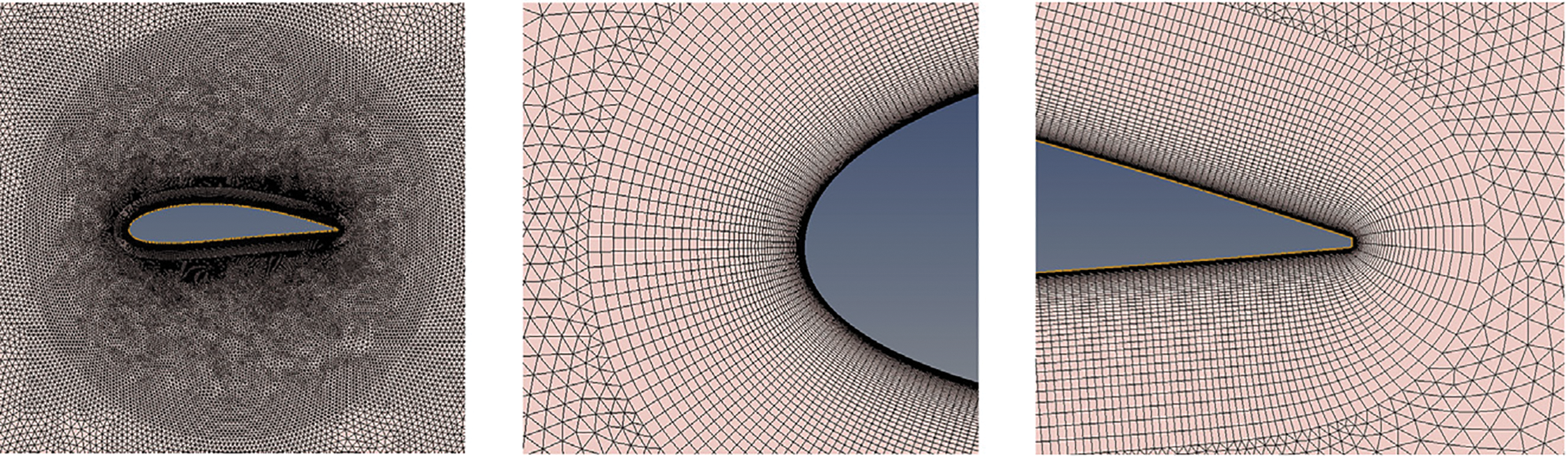
Figure 9: The hybrid mesh strategy, where the structured grids are used near the airfoil walls, and unstructured grids elsewhere in the domain [93]

3.3.2 Mesh Refinement and Independence

Beyond topology, the mesh density must be sufficient to capture high-gradient flow regions. This is achieved through mesh refinement, a process that is defined before the simulation begins (static refinement) and remains fixed. Refinement is targeted at areas where significant flow changes are anticipated, such as near blade surfaces, leading and trailing edges, and in the expected path of the wake. A critical verification step is to perform a mesh independence study, where simulations are run on a series of progressively finer meshes (e.g., coarse, medium, fine) to ensure that the solution (e.g., the power coefficient) no longer changes significantly with further refinement. This process is vital for quantifying the discretization error in the simulation. Several formal methods are used to assess this convergence:

•   General Richardson Extrapolation (GRE): GRE is a numerical method used to improve the accuracy of numerical solutions by combining results from solutions with different discretisation sizes. It effectively removes leading-order error terms, leading to higher-order accuracy [94]. In a study by [95], the GRE was applied to a regime of 2-D CFD simulations of VAWTs to monitor the power coefficient across different mesh resolutions. The technique provided a reliable measure of mesh convergence and helped identify flow phenomena such as vortex shedding and viscous losses, which are critical to turbine performance evaluation. In another study, GRE offered encouraging results for determining mesh-independent power coefficients in simulations of straight-blade VAWTs. Compared to exhaustive mesh refinement, GRE provided reliable results with lower computational cost [85]. Additionally, the GRE was successfully used to confirm mesh independence in dynamic stall simulations of a straight-blade VAWT. The study emphasised the importance of transition models for accurately capturing laminar separation bubbles, which significantly affect stall behaviour and turbine torque prediction [85].

•   Grid Convergence Index (GCI): GCI is a method used in CFD to estimate the accuracy of numerical results and assess their sensitivity to mesh discretisation. It helps to determine how much uncertainty is present in a simulation due to the mesh used, and if the results are converging towards a stable solution [96]. One of the most detailed studies by Almohammadi et al. evaluated four mesh independency techniques, i.e., mesh refinement, General Richardson Extrapolation (GRE), GCI, and a fitting method for a straight-blade VAWT. They found that while GRE was promising, GCI often failed to yield consistent results due to oscillations in the power coefficient convergence, making it unreliable in this context [85]. Despite its limitations, some studies still use GCI for initial mesh sensitivity analysis. For example, Liu et al. used GCI in assessing mesh convergence before evaluating aerodynamic performance improvements from a novel movable Gurney flap design on a VAWT [97].

3.3.3 Boundary Layer Meshing (i.e., Near-Wall Mesh Resolution, y+)

Accurately capturing the flow behaviour very close to the blade surfaces (the boundary layer) is critical for predicting forces (lift, drag, torque) and phenomena like separation and stall. This requires careful control of the mesh resolution perpendicular to the wall, often quantified by the non-dimensional wall distance, y+. It represents the distance of the first mesh cell centre from the wall, normalised by the viscous scales [98], as defined by Eq. (1).

y+=uτyν(1)

where uτ is the friction velocity as defined as

uτ=τωρ(2)

where y is the distance from the wall to the first cell center, 𝜈 is the kinematic viscosity, and 𝜏w is the wall shear stress.

The value of y+ needed depends heavily on the chosen turbulence model [68] or Low-RE models, such as Sheer Stress Transport (SST) k–ω or Transition SST (TSST), the turbulence model is designed to resolve flow structures down to the viscous sublayer, where viscous effects dominate [83]. Accurate application of these models typically requires very fine mesh resolution near the wall, with y+ values ideally around 1 or even below. Numerous VAWT CFD studies, considered as a general best practice, explicitly target y+< 1 or y+≈ 1 to ensure the boundary layer structure is adequately captured [71]. On the other hand, high-RE models using wall functions, commonly with standard k-ε models, coarser near-wall meshes with higher y+ values (e.g., y+ > 30) might be acceptable, but this approach models rather than resolves the near-wall flow, potentially reducing accuracy for separated flows [68]. Achieving the target y+ often requires generating multiple layers of thin, high-aspect-ratio cells (inflation layers or prism layers) adjacent to the wall surfaces [83]. Multiple studies use a y+ value greater than 30 in combination with wall treatment models like Spalart–Allmaras (SA) or URANS to balance accuracy and computational cost. This approach captures the near-wall flow structures without needing a fine mesh close to the wall, which would increase simulation time drastically [99,100].

VAWT simulations, especially those involving dynamic stall have shown that accurate capture of boundary layer development and separation requires finer near-wall resolution (y+ ≈ 1) for reliable torque and Cp prediction [84,101]. This is because boundary layer separation, and its timing during the blade’s azimuthal cycle, has a direct impact on the onset and intensity of dynamic stall [102]. Generating meshes that satisfy the stringent y+≈ 1 requirement necessitates using multiple thin, highly stretched “inflation” or “prism” layers adjacent to the wall. This significantly increases the total cell count, particularly in 3-D simulations, and contributes substantially to the overall computational cost. The choice between a low-Re approach (higher accuracy potential, higher cost) and a wall function approach (lower cost, potential accuracy limitations) represents a key decision in the simulation setup, driven by the specific goals and available resources [54,103].

3.3.4 Moving Mesh Techniques

As discussed, VAWTs operate in a complex aerodynamic environment, where the angle of attack on VAWT blades changes continuously throughout each rotation. Capturing the transient effects associated with VAWTs requires time-accurate CFD simulations where the turbine’s rotation is explicitly modelled [104]. One of the key parameters influencing the stability and accuracy of such unsteady simulations is the Courant–Friedrichs–Lewy (CFL) number, defined as:

CFL=uΔtΔx(3)

where u is the local flow velocity, Δt is the time step, and Δx is the characteristic mesh length scale. In transient VAWT simulations, maintaining CFL ≤ 1 is typically recommended to ensure numerical stability, particularly when resolving sharp gradients near blade surfaces and wake regions. Lower CFL values (e.g., 0.1–0.5) are often necessary for accurate prediction of dynamic stall and vortex shedding phenomena, especially when using sliding mesh methods. This stability criterion is well established in CFD literature [105]. Numerical studies focusing on rotating and sliding mesh in VAWTs, such as the work by Trivellato and Raciti Castelli (2014), have emphasized the importance of strict CFL control at interface zones to ensure accurate torque and power coefficient estimation [106]. This is where moving mesh techniques come in. Three common mesh motion strategies used in simulating rotating components like wind turbine blades are sliding mesh, overset mesh, and morphing mesh, each offering distinct approaches to handling relative motion between rotating and stationary domains.

•   Sliding mesh (or sliding grid): The most common technique for simulating rotating machinery is the sliding mesh approach [83]. This technique is designed to handle the relative motion between rotating and stationary components, making it highly suitable for VAWT simulations. The computational domain is explicitly divided into at least two cell zones: a rotating zone containing the turbine rotor and a stationary zone representing the surrounding environment (as shown in Figs. 6 and 7). These zones meet at one or more interface boundaries. The mesh within the rotating zone is physically rotated at the specified turbine speed relative to the stationary zone mesh at each time step. Specialised CFD algorithms are required to identify intersecting faces and accurately interpolate values between non-matching cells to compute mass, momentum, and energy fluxes across the interface at each time step [77,107]. The sliding mesh technique has proven effective for simulating VAWT rotation, showing good agreement with experiments in studies using models like the straight-bladed NACA0021, VAWT with flat plate deflectors [108], twin VAWT configurations validated against experiments [109] and variable blade pitching increasing performance by 81% at certain tip speed ratios [110] with satisfactory alignment with experimental data. Advanced applications of the sliding mesh technique include the integration of passive flow control mechanisms [111] and the effects of dielectric barrier discharge plasma actuators, which improved the power coefficient by 38% compared to conventional fixed-pitch VAWTs [112]. The sliding mesh technique offers several advantages for CFD simulations, including ease of implementation in most codes, natural handling of large rotational motions, and the ability to maintain good mesh quality within each rotating zone through rigid body motion [113]. However, it requires careful setup of interface boundaries, and interpolation across the non-conformal interface can introduce numerical errors, though these are generally minimal with adequate mesh resolution. Maintaining mesh quality near the interface is crucial, and since the method relies on an unsteady simulation framework with time-step interface calculations, it is more computationally demanding than steady-state approaches like the Multiple Reference Frame (MRF) method, which is less suited to the inherent unsteadiness of VAWTs [114].

•   Overset mesh (or Chimaera mesh/overlapping grid): The overset mesh technique, also known as Chimaera grids, offers an alternative approach for handling relative motion and complex geometries. This technique uses multiple independent meshes that overlap geometrically. A “component” mesh containing the VAWT blades moves through a stationary “background” mesh representing the far-field. Cells in the overlapping regions communicate via interpolation (graphically shown in Fig. 10). Special algorithms identify active cells, inactive cells within the background mesh covered by the component mesh, and interpolation cells at the overlap boundary [115]. The overset mesh technique is prominently used to simulate the dynamic motion of floating vertical axis wind turbines (OF-VAWTs) under various degrees of freedom. This approach helps in understanding how surge motion affects the aerodynamic performance and stability of the turbines [116]. The overset mesh allows for capturing complex flow interactions around the rotor blades, which are crucial for optimising turbine design and performance under varying wave loads [117]. In the context of Savonius wind turbines, the overset mesh framework has been used to simulate wind-driven rotation and assess modifications in blade design. This approach has demonstrated potential improvements in power efficiency by 10%–28% [118]. While sliding mesh is often more efficient in simpler cases, overset mesh handles more complex and flexible movements better [91]. It also simplifies meshing by allowing separate meshing of complex components like blades, independent of the background mesh, enabling non-traditional blade motion [119]. However, it requires careful setup of overlapping regions and interpolation schemes, with accuracy depending on mesh resolution in these areas. Poor overlap or resolution can cause significant errors or conservation issues, and robust algorithms are needed to manage potential orphan cells that lack interpolation data [120].

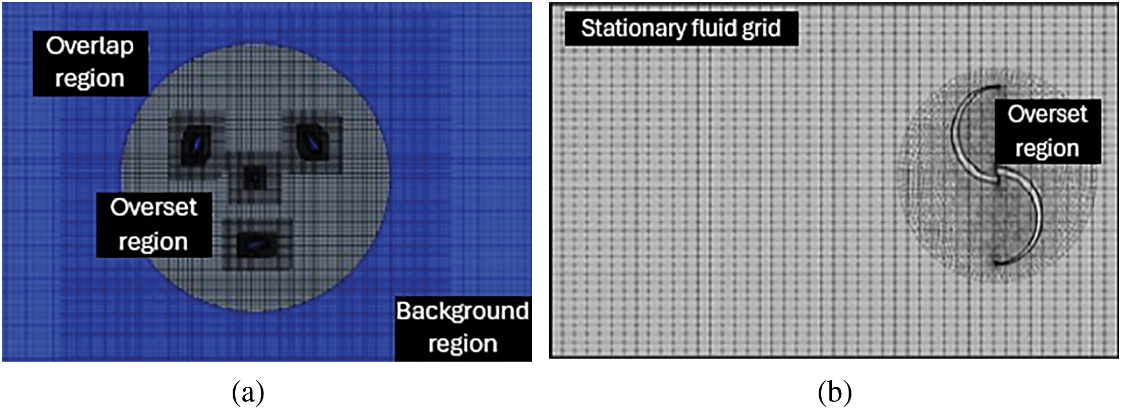
Figure 10: (a) Computational mesh topology showing the overset and overlap regions (image cropped from [116]), and (b) a structured background mesh overlapping with an unstructured but layered mesh around the turbine in the overset region (image cropped from [118])

•   Morphing mesh (or deforming mesh/dynamic mesh): This strategy involves adapting the mesh to accommodate boundary motion or deformation beyond the rigid body rotation handled by sliding or overset methods. They are particularly relevant for simulating Fluid-Structure Interaction (FSI) or turbines with actively deforming components like morphing blades [65,121–123]. The mesh connectivity (or the topology) of the morphing mesh technique remains constant during rotation of the blades, but the nodes of the mesh move to accommodate the boundary motion. The motion of the internal mesh nodes is typically calculated using algorithms like spring-based smoothing, diffusion-based smoothing, or remeshing techniques when distortion becomes too severe [123,124]. In a study that introduced a novel design for VAWTs that employs a blade morphing technique, the researchers dynamically adjust the blade shape based on azimuthal angle and TSR. This approach uses a Free-Form Deformation (FFD) algorithm combined with a mesh morpher and optimisation methods, leading to significant improvements in power output compared to fixed-blade designs [125]. As shown in Fig. 11, the researchers created control points to set the scale and direction of deformations. These points keep proper connectivity between deforming and non-deforming regions. The morphing mesh technique’s main advantage is that it preserves mesh topology, avoiding interpolation errors common in sliding or overset methods. It is especially well-suited for modelling structural deformations and fluid–structure interaction (FSI) problems where boundary movements are small relative to cell size [65,121]. However, it is not suitable for large, rigid body motions like full VAWT rotation, as this can severely distort the mesh and degrade quality. It also requires strong algorithms to move internal nodes without creating invalid cells, and frequent remeshing to correct distortion can be both computationally costly and prone to interpolation errors [65,124,126].

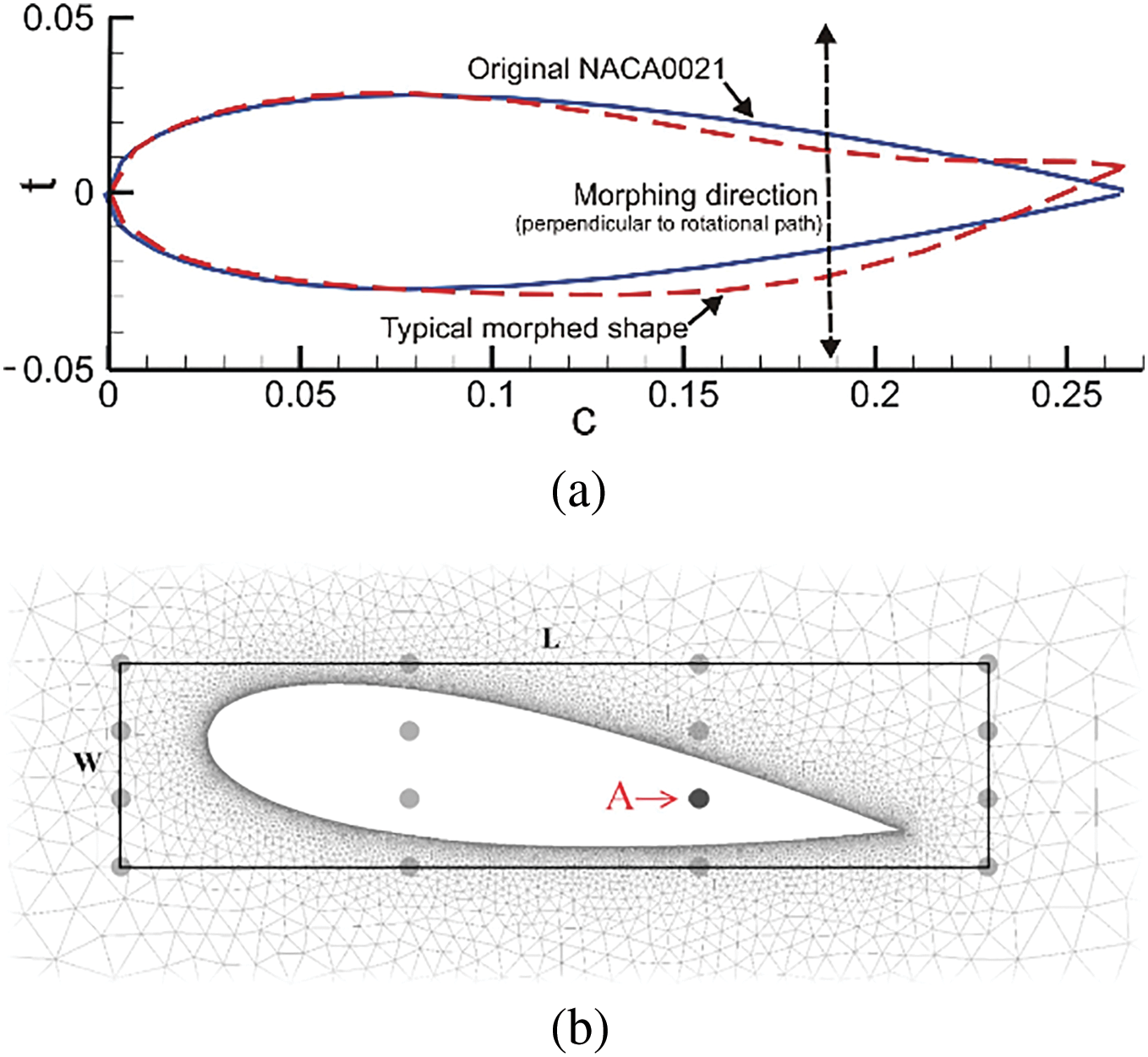
Figure 11: (a) NACA0021 unaltered shape profile vs. (a) NACA0021 morphed shape profile, and box encasement for the blade showing the control points [125]

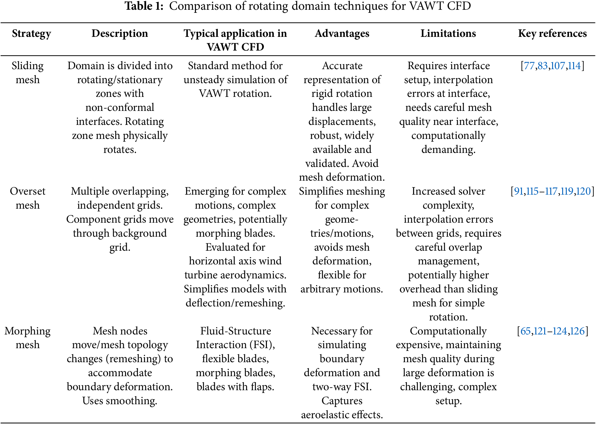
Table 1 provides a comparison of sliding mesh, overset mesh, and morphing mesh strategies, highlighting their descriptions, advantages, and disadvantages in the context of simulating rotating systems.

3.3.5 Mesh Quality Metrics

Beyond mesh density and near-wall resolution, the overall quality of the mesh elements significantly impacts simulation stability, convergence speed, and solution accuracy. Poorly shaped cells can introduce large discretisation errors [77,127]. Key metrics used to assess mesh quality include:

•   Skewness: Measures the deviation of a cell from its ideal shape (e.g., equilateral triangle, square, regular tetrahedron/hexahedron). High skewness is generally undesirable. A maximum skewness target might be set during meshing [77].

•   Aspect ratio: The ratio of the longest edge or dimension of a cell to its shortest. High aspect ratios are acceptable and often necessary in boundary layers (where cells are stretched parallel to the wall) but can be problematic in isotropic flow regions.

•   Orthogonality: Measures the angle between cell faces and the vectors connecting cell centroids. Low orthogonality (high non-orthogonality) can degrade accuracy, especially for pressure-velocity coupling schemes.

•   Smoothness/growth rate: Refers to the rate at which cell size changes between adjacent cells. Abrupt changes in cell size can lead to numerical errors. A gradual transition is preferred [128].

•   Mesh size: The total number of cells can vary widely depending on the dimensionality (2-D vs. 3-D), geometric complexity, required resolution, and simulation type (Reynolds-averaged Navier–Stokes, or RANS vs. SRS). There is no standard for determining the most optimal mesh size for a VAWT CFD, since every numerical model will differ. Examples range from hundreds of thousands for 2-D Unsteady-RANS 36 to over 10 million for detailed 3-D RANS/SRS simulations [83]. Farm simulations involving multiple turbines naturally require even larger meshes [76].

CFD software packages typically provide tools to diagnose mesh quality based on these metrics. It is standard practice to check and improve mesh quality during the generation process to ensure it meets acceptable standards before proceeding with the simulation. The selection of domain size, mesh topology, near-wall resolution strategy, and turbulence model is intrinsically linked. For example, opting for a low-Re turbulence model necessitates achieving y+≈ 1, which significantly increases the mesh density near walls. This heightened cell count might compel the modeller to reduce the overall domain size or limit the simulation to 2D or 2.5D to maintain a manageable total computational cost, despite the known importance of 3-D effects and large domains for minimising boundary influence. Conversely, choosing a wall function approach relaxes the y+ constraint, potentially enabling larger domains or 3-D simulations within the same cost envelope, but at the risk of lower accuracy for boundary layer dominated phenomena like stall. While general guidelines for parameters like domain size (e.g., 10D upstream/downstream, 20D width) and y+ (e.g., < 1 for low-Re models) are valuable starting points and represent emerging best practices, the optimal configuration is highly dependent on the specific VAWT geometry, its operating regime (TSR), the physical phenomena under investigation (e.g., peak performance vs. dynamic stall vs. wake interactions), and the chosen numerical schemes.

Consequently, sensitivity studies examining the impact of these parameters remain crucial for ensuring the reliability of VAWT CFD simulations. To further illustrate mesh sensitivity, Fig. 12 presents the variation of the moment coefficient (Cm) over one turbine revolution, comparing medium and fine mesh resolutions at a fixed time step of 0.0002 s. The figure is taken from Naidu et al. (2019), demonstrate that both mesh levels yield consistent aerodynamic behavior, with the fine mesh producing a smoother Cm profile [129]. This supports the mesh convergence assumption and confirms that medium mesh resolution is sufficient for capturing key unsteady flow features in 2-D VAWT simulations.

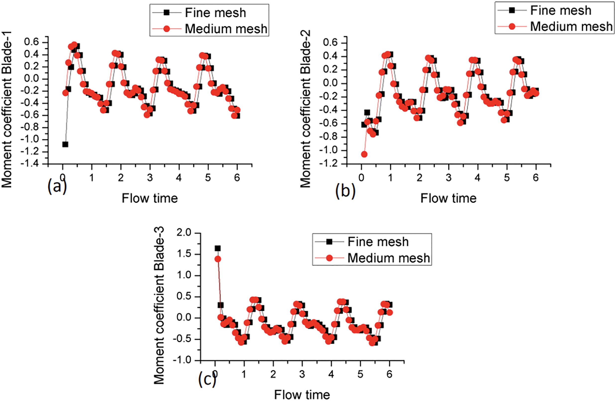
Figure 12: Instantaneous moment coefficient (Cm) of Blade 1 plotted over one full rotation (azimuth angle θ), comparing medium and fine mesh resolutions at a time step of 0.0002 s [129]

3.4 Turbulence Modelling Approaches in CFD and Their Applications in VAWT Analysis

3.4.1 The Nature of Turbulence in VAWT Flows

Turbulence represents a pervasive phenomenon within fluid dynamics, characterised by chaotic, irregular, and stochastic fluid motion occurring across diverse spatial and temporal scales [130]. Within the operational context of VAWTs, turbulence manifests through multiple mechanisms. The ambient atmospheric wind frequently exhibits turbulent properties, particularly in urban environments or complex topographical settings where VAWTs are commonly deployed [65,69]. This upstream turbulence subsequently interacts with the turbine rotor structure. Furthermore, the fluid flow surrounding the rotating blades develops turbulent characteristics as boundary layers form, potentially separate, and undergo transition from laminar to turbulent regimes [70,131]. The wakes generated by the blades, structural components, and the complete rotor assembly inherently display turbulent properties, containing complex vortical structures [68,71].

A fundamental attribute of turbulent flows is the energy cascade mechanism: large-scale eddies, which contain the majority of kinetic energy, progressively fragment into smaller eddies, facilitating energy transfer across scales until reaching the Kolmogorov microscales, where viscous dissipation transforms kinetic energy into thermal energy [132]. The principal challenge in Computational Fluid Dynamics (CFD) turbulence modelling accurately represents the effects of this multi-scale phenomenon on mean flow properties, including velocity distributions, pressure fields, and aerodynamic force coefficients [133]. Although Direct Numerical Simulation (DNS), which resolves all turbulent scales to the Kolmogorov scale, provides a comprehensive characterisation of turbulent flow behaviour, its computational requirements increase prohibitively with Reynolds number, rendering it impractical for applied engineering applications such as VAWT simulation [95]. Consequently, alternative modelling methodologies are implemented to render turbulent flow simulations computationally feasible.

The transition from laminar to turbulent flow can be predicted through analysis of the dimensionless Reynolds number (Re), which quantifies the ratio between inertial and viscous forces within a fluid (i.e., Re=ρνL/μ, where ρ represents fluid density,v denotes characteristic velocity, L indicates characteristic length, and μ is the dynamic viscosity of the fluid). Turbulent flow typically emerges when the Re exceeds critical thresholds specific to the flow configuration and boundary conditions [134].

3.4.2 Reynolds-Averaged Navier-Stokes (RANS/URANS)

The most widely used approach for industrial CFD simulations is based on the Reynolds-Averaged Navier-Stokes (RANS) equations, as shown in Eq. (4). This method decomposes the instantaneous flow variables into a mean (time-averaged or ensemble-averaged) component and a fluctuating component. Substituting these into the Navier-Stokes equations and averaging leads to equations for the mean flow that resemble the original equations but contain an additional term known as the Reynolds stress tensor [135,136]. This tensor represents the effects of turbulent fluctuations on the mean flow.

ρ(∂u¯i∂t+u¯j∂u¯i∂xj)=−∂p¯∂xi+µ∂2u¯i∂xj2−∂∂xj(ρui′uj′¯)(4)

The core task of RANS turbulence modelling is to provide a mathematical model for the unknown Reynolds stresses to close the system of mean flow equations. The most common approach relies on the Boussinesq hypothesis, which relates the Reynolds stresses to the mean velocity gradients via an eddy or turbulent viscosity [135]. Models that use this hypothesis are called eddy viscosity models. Among these, two-equation models are prevalent, which solve transport equations for two turbulence quantities to determine the eddy viscosity. The most common pairs are k-ε models and k-ω models [95,135]. For inherently unsteady flows like those around VAWTs, the Unsteady RANS (URANS) formulation is used, where the averaging is performed over ensembles rather than time, but the fundamental modelling challenge remains the same [136–139]

A fundamental limitation of the RANS/URANS approach is that it models the effect of all turbulent scales on the mean flow. It does not resolve any part of the turbulence spectrum directly. This time- or ensemble-averaging process can inherently smear out large-scale, unsteady turbulent structures that might be physically important, particularly in flows with massive separation or strong vortex shedding, such as those encountered during dynamic stall on VAWT blades [70,140]. While computationally efficient, this limitation can compromise the accuracy of RANS/URANS models for flows where the dynamics of large turbulent eddies play a dominant role. This section delves into the performance and applicability of specific RANS/URANS turbulence models commonly encountered in VAWT CFD simulations, evaluating them based on findings from the literature.

•   k-ε family: The k-ε family of two-equation models solves transport equations for the turbulent kinetic energy (k) and its rate of dissipation (ε). While historically popular in CFD due to their robustness and computational efficiency for certain classes of flows, their suitability for VAWT simulations is highly questionable. The standard k-ε model, the oldest and simplest in this family, uses wall functions to bridge the viscous sublayer near walls, thus avoiding the need for extremely fine mesh resolution close to the wall. It is governed by the following transport equations:

Turbulent kinetic energy (k) equation:

ρ(∂u¯i∂t+u¯j∂u¯i∂xj)=−∂p¯∂xi+µ∂2u¯i∂xj2−∂∂xj(ρui′uj′¯)(5)

Turbulent dissipation rate (ε) equation:

∂ε∂t+uj∂ε∂xj=Cε1εkPk−Cε2ε2k+∂∂xj((ν+νtσε)∂ε∂xj)(6)

Despite this computational convenience, it is generally regarded as unsuitable for accurately simulating VAWT aerodynamics due to poor performance in flows with strong adverse pressure gradients, inaccurate prediction of flow separation, and the limitations of standard wall functions [62,95,135]. Extensive comparative studies consistently show that it fails to reproduce VAWT performance metrics accurately [137,141]. While the model is computationally efficient, it provides low accuracy in the context of VAWT applications.

•   RNG k-ϵ model: The model was developed using Renormalisation Group (RNG) theory, modifies the ε-equation and adjusts model constants to enhance performance in swirling flows and to accommodate low-Re effects. While intended to offer improvements over the standard model, the RNG k-ε model is also generally found to perform poorly in VAWT simulations, particularly in predicting the power coefficient (Cp) [137].

•   Realisable k-ϵ model: The model introduces a modified transport equation for ε based on the mean square vorticity fluctuation and incorporates mathematical constraints (realizability) to ensure the positivity of normal stresses and adherence to the Schwarz inequality for shear stresses, which are not guaranteed in the standard model. Despite these theoretical advancements, the Realisable k-ε model continues to struggle with the aerodynamic complexities of VAWT flows [137]. Comparative studies have shown that it yields substantial errors in Cp prediction, sometimes underestimating and sometimes overestimating, with high root mean square errors and mean average percentage errors compared to experimental data or transitional models [138,142]. Overall, it offers low to moderate accuracy at a similarly low computational cost [137,142].

•   k-ω family: The k-ω family of models solves transport equations for turbulent kinetic energy (k) and the specific dissipation rate (ω, proportional to ε/k). These models generally offer advantages over k-ε models, particularly in the near-wall region. The one originally developed by Wilcox [143], the standard model can be integrated directly to the wall without the use of wall functions, providing improved near-wall accuracy. However, it is sensitive to freestream ω values and less robust than its more commonly used variant, the SST k-ω model. While less frequently applied in VAWT studies, it forms the foundation for advanced models like the Scale Adaptive Simulation (SAS) and the Stress-Blended Eddy Simulation (SBES) [137,139,144]. To mathematically describe the model, the governing equations of the standard k-ω formulation are:

Turbulent kinetic energy (k) equation:

∂k∂t+uj∂k∂xj=Pk−β∗kω+∂∂xj[(ν+σkνt)∂k∂xj](7)

Specific dissipation rate (ε) equation:

∂ω∂t+uj∂ω∂xj=α(ωk)Pk−βω2+∂∂xj[(ν+σωνt)∂ω∂xj](8)

•   SST k-ω model: The model introduced by Menter [145], is a highly popular and effective two-equation model that blends the strengths of k-ω and k-ε models using a blending function to achieve accurate near-wall predictions and robust freestream behavior [69,136]. It includes a shear stress transport limiter that helps simulate adverse pressure gradients and flow separation more accurately [69]. The SST k-ω model is widely regarded as one of the most suitable and reliable RANS/URANS models for VAWT simulations [62,69,83,131,142], which demonstrated the capability to predict power coefficients and torque accurately, which are critical for turbine design and optimisation [108,146–148]. Its formulation provides good performance for both attached and separated flows, offering significantly better prediction of flow separation compared to k-ε models [92,131,137]. Numerous studies report that SST k-ω can provide reasonable agreement with experimental data for Cp, Ct, and wake characteristics across various TSRs, although the level of accuracy can vary depending on the specific case and simulation setup [61,68,131,136,142,149]. While it generally performs well without explicit transition modelling [69], its accuracy in low-to-moderate TSR regimes can be improved by incorporating transition models [137,131,142]. It may also underpredict the severity of deep dynamic stall compared to transitional or hybrid models [137] and results can vary with simulation dimensionality (2-D vs. 3-D) [69,130,131].

•   Spalart-Allmaras (SA): The SA model is a one-equation turbulence model that solves a single transport equation for a modified turbulent kinematic viscosity (ν~) [95,135,136]. Originally developed for external aerodynamic flows in the aerospace industry, particularly for attached boundary layers on airfoils and wings. The model computes the eddy viscosity from ν~ using the relation:

νt =ν~fv1(9)

where fv1 is a viscous damping function,and defined as:

fv1=χ3(χ3+Cv13),χ=ν~ν(10)

where ν is a molecular kinematic viscosity, and Cv1 is a model constant. The governing equation for ν~ is given by:

∂ν~∂t+uj∂ν~∂xj=Cb1(1−ft2)ν~s˙+(1σ)[∂∂xj((ν+ν~)∂ν~∂xj)+Cb2(∂ν~∂xj)2]−Cw1fw(ν~d)2(11)

where the constants Cb1, Cb2, Cw1, and σ are model coefficients.

The SA model is significantly more computationally efficient than two-equation models. This efficiency has led to its occasional use in vertical axis wind turbine (VAWT) simulations, where some studies have reported reasonable agreement in capturing dynamic stall behavior despite the model’s simplicity [83]. However, its overall performance in VAWT applications is limited. Validation studies consistently show that the SA model performs poorly in predicting key aerodynamic outputs such as power and torque coefficients (Cp, Ct) and wake development [95,135,137]. It is generally less accurate than more advanced two-equation models like SST k-ω, particularly in resolving flow separation [135]. Overall, it offers very low computational cost but at the expense of low predictive accuracy for VAWT performance [95,137].

•   Transitional models (focusing on SST variants): Boundary layer transition plays a critical role in the aerodynamics of small to medium-sized VAWTs, especially at low tip speed ratios (TSRs), where local Reynolds numbers typically range from 105 to 106 [131,137,142]. In this regime, much of the blade surface may remain laminar before transitioning to turbulence, influencing separation, dynamic stall, and aerodynamic performance. Standard RANS models like k-ϵ and SST k-ε assume fully turbulent flow and cannot capture the gradual laminar-to-turbulent transition [131,137,142]. This limitation motivates the use of specialised transitional turbulence models. The most widely used is the Transition SST (TSST) or γ–Reθt model, a four-equation model that combines SST k-ω with two additional equations for intermittency (γ) and transition momentum thickness Reynolds number (Reθt) [62,68,137,138,142]. The γ variable triggers turbulence generation only downstream of the predicted transition point, enabling more realistic boundary layer modeling [142]. TSST improves predictions of power and torque coefficients, especially at low-to-moderate TSRs, and captures phenomena like laminar separation bubbles and dynamic stall vortices more effectively than standard SST k-ω [131,137,138,142]. Additionally, the transition SST model’s performance is also affected by the uncertainty in wall distance calculations, which can impact the accuracy of turbulence/transition predictions [150]. However, its performance is sensitive to simulation parameters such as mesh resolution, azimuthal increment, and inlet turbulence conditions.

A related approach, SST k-ω with intermittency (SSTI), uses a γ equation within a slightly simplified formulation. While offering similar transitional modeling capabilities, results can vary depending on implementation. In some cases, SSTI predicted laminar separation bubbles but showed unphysical behavior or poorer agreement with pressure data compared to SST k-ω [62,137]. Another transitional model, the k-kl-ω, solves for transport turbulent kinetic energy, laminar kinetic energy, and ω, aiming to capture transition via Tollmien-Schlichting instabilities. However, it has shown poor performance for VAWTs in comparative studies.

The literature evidence indicates that the Transition Shear Stress Transport (TSST) model and its variants demonstrate enhanced predictive capability compared to conventional Reynolds-Averaged Navier-Stokes (RANS) models for Vertical Axis Wind Turbine (VAWT) simulations [78,137]. Phenomena like dynamic stall, which significantly influence VAWT torque production, involve complex boundary layer dynamics where the state of the boundary layer prior to separation plays a crucial role. By assuming fully turbulent flow, Standard RANS models inherently miss this critical piece of physics. The TSST model, by explicitly modelling intermittency and transition onset, provides a more physically realistic representation of the boundary layer development, leading to improved predictions of stall onset, vortex shedding dynamics, and overall turbine performance [78,137,142,151,152].

3.4.3 Scale-Resolving Simulation (SRS) Models

Scale-Resolving Simulation (SRS) models offer a higher-fidelity approach. Unlike RANS, which models the effect of all turbulent scales on the mean flow, SRS models aim to directly resolve the larger, energy-containing turbulent eddies while modelling only the smaller, more universal scales. This category includes Large Eddy Simulation (LES), Detached Eddy Simulation (DES), and related hybrid RANS-LES approaches like Scale-Adaptive Simulation (SAS), Improved Delayed DES (IDDES), and Stress-Blended Eddy Simulation (SBES).

•   Large Eddy Simulation (LES): LES offers a higher-fidelity approach than RANS/URANS. The fundamental idea behind LES is to directly resolve the large, energy-containing turbulent eddies in the flow field while modelling the effects of the smaller, more universal sub-grid scale (SGS) eddies [70,83,95,138,139]. This is achieved by applying a spatial filter to the Navier-Stokes equations, which separates the large, resolved scales from the small, unresolved (sub-grid) scales [153]. The main advantage of LES is its potential to capture the unsteady dynamics of large turbulent structures much more accurately than RANS/URANS [70]. This is particularly relevant for VAWTs, where dynamic stall vortex shedding and wake evolution involve large, coherent turbulent structures. However, this increased fidelity comes at a significantly higher computational cost [70,138,139]. LES requires much finer computational meshes than RANS/URANS to resolve a sufficient range of turbulent scales. Additionally, LES simulations must be run as unsteady calculations with small time steps to capture the temporal evolution of the resolved eddies [154]. Due to these high costs, pure LES is often restricted to fundamental research, benchmarking studies, or simulations of relatively simple geometries or low-Re flows [70,140].

•   Hybrid RANS-LES models: Hybrid RANS-LES models have emerged as a pragmatic approach seeking to bridge the gap between the computational efficiency of RANS/URANS and the high fidelity of LES [95,138–140,155]. The core idea is to combine the strengths of both methods: use the computationally cheaper RANS approach to model the flow in regions where it performs adequately (typically attached boundary layers near walls, where LES is most expensive) and switch to an LES-like approach to resolve the large, unsteady turbulent structures in regions where RANS struggles (typically separated flow regions, wakes, and free shear layers) [138–140]. Several hybrid strategies have been developed, i.e., Detached Eddy Simulation (DES) [95,140], Delayed DES (DDES) and Improved DDES (IDDES) DES [64,82,137,139,140,155], Scale-Adaptive Simulation (SAS) [95], and Stress-Blended Eddy Simulation (SBES) [138,139]. This aims to provide a more robust and rapid transition between the RANS and LES zones compared to DES-type switching mechanisms. These models aim to efficiently capture complex, separated turbulent flows typical in VAWTs, where standard RANS lacks fidelity and LES is often too costly [70,140]. The evolution from DES to SBES reflects ongoing efforts to balance accuracy and computational cost while resolving key unsteady features like dynamic stall and wake dynamics [95,138,140].

3.4.4 Summary and Recommendations

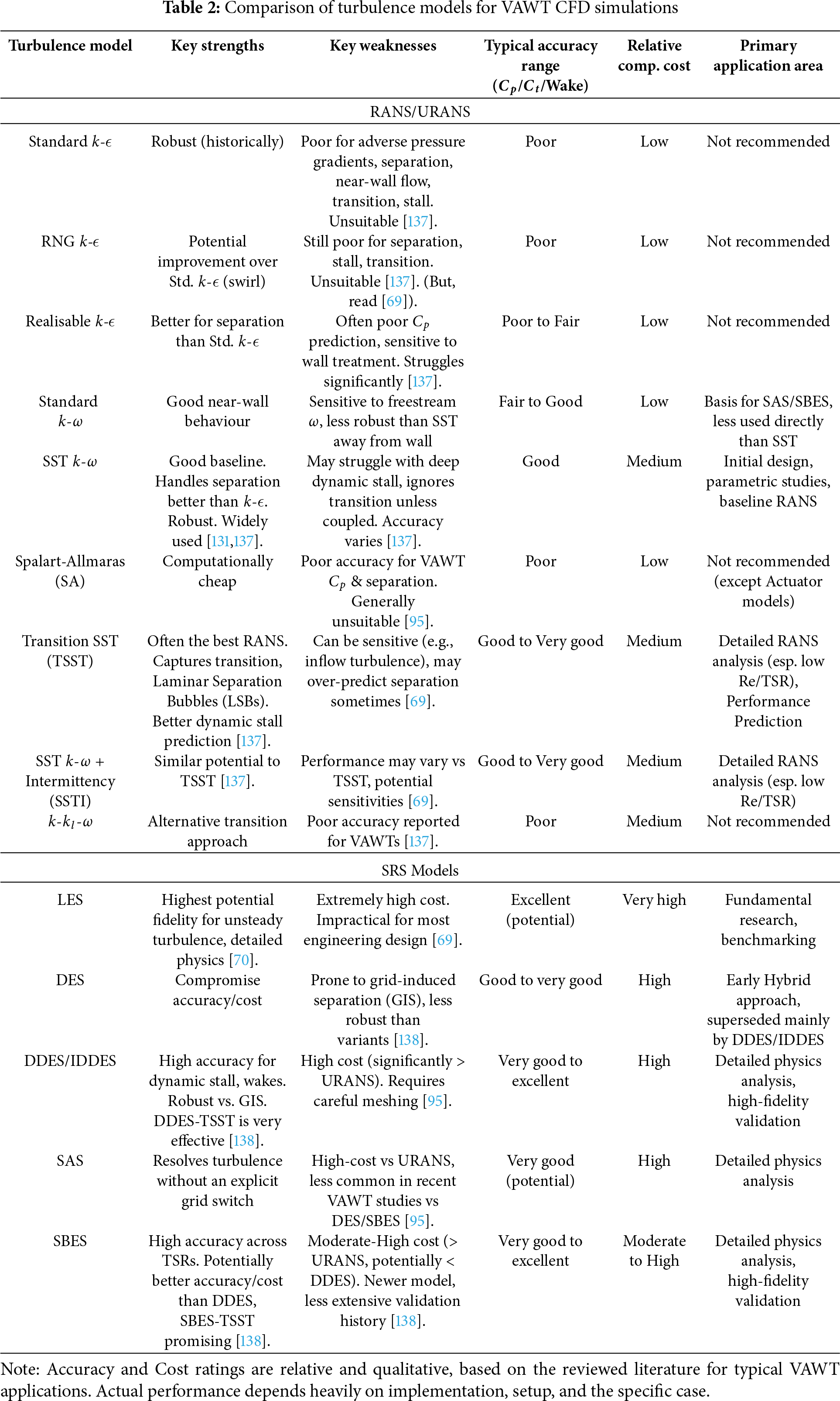
This section synthesises the findings of the previous analyses, directly comparing the turbulence models and offering guidance for model selection based on specific simulation objectives and constraints. Table 2 summarises the turbulence models discussed, evaluating them against key criteria relevant to VAWT CFD simulations. Accuracy ratings are qualitative (Poor, Fair, Good, Very Good, Excellent) based on the consensus from the reviewed literature for predicting overall performance (Cp, Ct) and key flow features (stall, wake). Cost ratings are relative (Low, Medium, High, Very High).

The selection of a turbulence model for VAWT CFD invariably involves a trade-off between the desired level of predictive accuracy and the available computational resources (time and hardware). Fig. 13 illustrates this relationship conceptually. At the lower end of the cost spectrum lie the standard RANS/URANS models. While computationally inexpensive, models like the k-ε family and Spalart-Allmaras generally offer poor accuracy for VAWTs [137]. The SST k-ω model represents a significant increase in accuracy for a moderate increase in cost, providing a reasonable baseline. Incorporating transition modelling, primarily through the TSST model, further enhances accuracy, particularly for capturing stall and transitional effects critical at lower Re/TSRs, at the cost of solving additional transport equations (roughly 25%–35% cost increase over SST k-ω as reported by [138]). Moving towards higher fidelity requires resolving parts of the turbulent spectrum, leading to significantly increased computational demands. Hybrid RANS-LES models like DDES, IDDES, SAS, and SBES offer substantial improvements in capturing unsteady flow physics, dynamic stall intricacies, and wake structures compared to URANS [138–140,155]. However, this comes at a considerable cost premium. DDES/IDDES simulations, for instance, have been reported to require roughly 4.5 times the computational time of a TSST simulation [138]. SBES appears potentially more efficient, with reported costs closer to 1.5 times that of TSST in one study, while still delivering accuracy comparable to or better than DDES/IDDES [138]. At the far end of the spectrum, LES offers the highest potential fidelity but with computational costs that are often prohibitive for practical engineering timescales [70].

Figure 13: Conceptual illustration of the Accuracy vs. Computational Cost trade-off for turbulence models in VAWT CFD

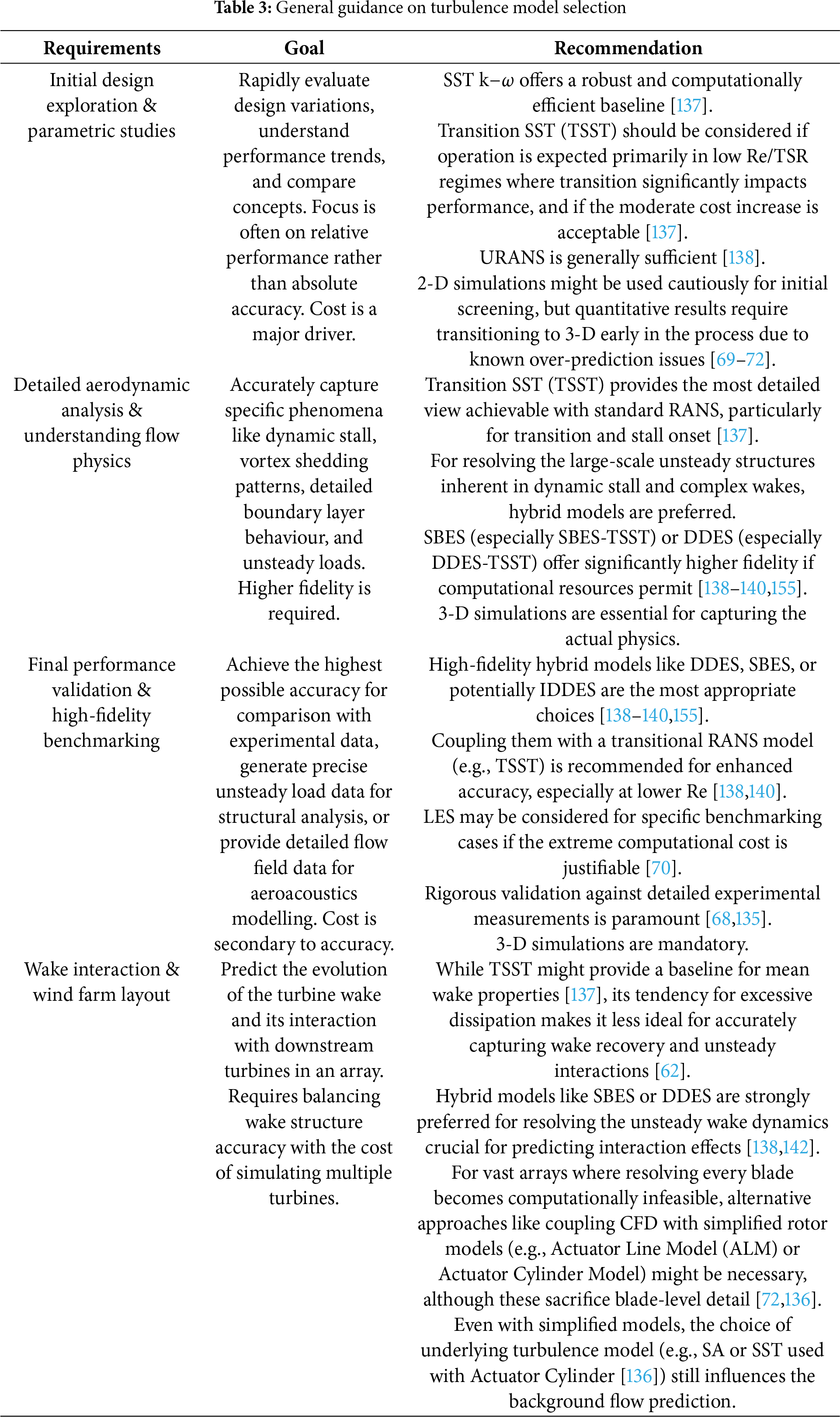
Different turbulence models exhibit varying capabilities in capturing the specific aerodynamic phenomena crucial to VAWT operation, e.g., dynamic stall, flow separation, tip vortices and 3-D effects, wake characteristics and transitional flow. The optimal choice of turbulence model depends heavily on the CFD simulation’s specific goals, the required accuracy level, and the available computational resources. The following Table 3 encapsulates the general guidance on turbulence model selection.

3.5 Solver Configuration and Convergence Practices

Appropriate solver settings are crucial for obtaining stable and accurate transient solutions for VAWTs.

•   Solver Type: For the relatively low Mach numbers typical of wind turbine applications, pressure-based solvers are commonly employed [82].

•   Discretisation Schemes: Using at least second-order accurate schemes for both spatial and temporal discretisation is generally recommended to minimise numerical diffusion and accurately capture transient phenomena [68,83].

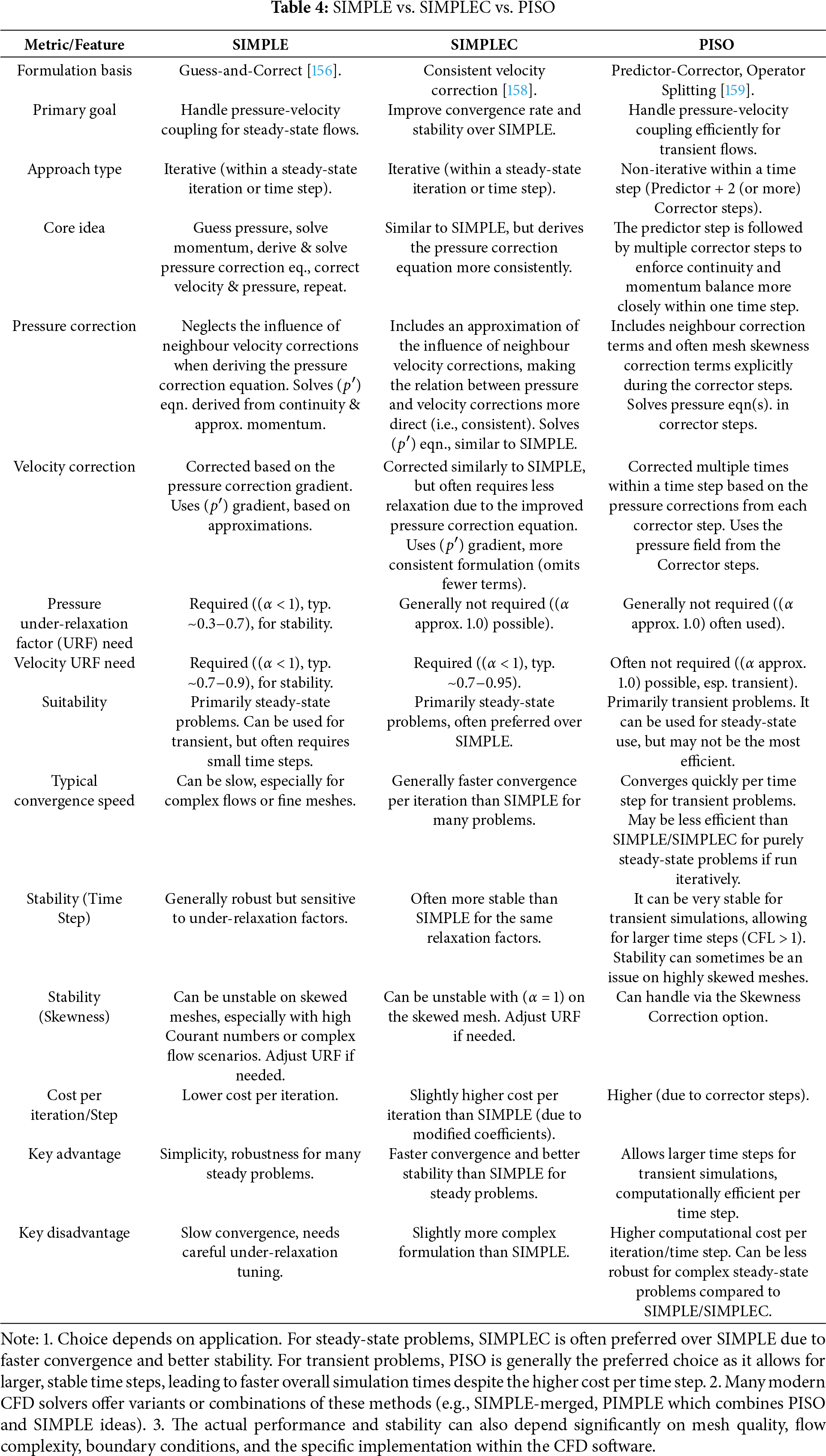
•   Pressure-Velocity Coupling: Algorithms like SIMPLE (Semi-Implicit Method for Pressure Linked Equations) [156,157], SIMPLEC (SIMPLE-Consistent) [158], or PISO (Pressure-Implicit with Splitting of Operators) [159] are used to handle the interdependence of pressure and velocity in the governing equations [68,83]. Table 4 summarises the key characteristics and comparative aspects between these algorithms.

•   Time Stepping: Transient simulations are required since VAWT flow is inherently unsteady. The time step size (Δt) must be small enough to resolve the relevant timescales of the flow, including blade passage, vortex shedding, and dynamic stall evolution. It is often convenient to define the time step based on the desired azimuthal increment (dθ), i.e., the turbine rotates per step (Δt=dθ/Ω, where Ω is the rotational speed in rad/s) [68].

The required dθ is highly dependent on the TSR and the complexity of the flow [68]. Studies indicate that for moderate to high TSRs (e.g., λ > 3.5–4.5) where flow is largely attached, dθ = 0.5° or even 1.0° might suffice [68]. However, for low to moderate TSRs where dynamic stall and complex blade-wake interactions dominate, or for low Reynolds number flows, a much finer resolution of dθ = 0.1° is often necessary to accurately capture these phenomena [68,76].

•   ○ Within each time step, multiple inner iterations (e.g., 10–50) are typically needed to converge the nonlinear algebraic equations before advancing to the next time step [68,83].

Initialisation and Convergence: Transient simulations are often initialised using a converged steady-state RANS solution to provide a reasonable starting flow field and potentially reduce the time needed to reach a periodic state [68]. The simulation must then be run sufficiently long to allow initial transients to dissipate. Monitoring key performance indicators like blade torque or overall power coefficient over successive revolutions is crucial. A statistically steady (periodic) state is typically considered reached when these metrics exhibit consistent cycle-to-cycle behaviour [68]. Studies suggest that 20 to 30 complete turbine revolutions may be required to achieve this state before meaningful time-averaged performance data can be extracted [160], with convergence criteria of between 10−4 to 10−5 [137].

Achieving reliable CFD results for VAWTs demands a careful, integrated approach. The choices of turbulence model, mesh resolution (particularly y+), and time step size are interconnected [68]. For instance, resolving the boundary layer with a low-y+ mesh using an appropriate turbulence model (like SST) often necessitates smaller time steps to maintain stability and capture unsteady near-wall events accurately. While guidelines and best practices exist (summarised in Table 5), significant expertise is required for proper setup, execution, monitoring of convergence, and subsequent validation against experimental data. The apparent ease of using modern CFD software can mask the considerable underlying effort needed to produce trustworthy results for these challenging flow problems.

3.6 Summary of Methodological Choices

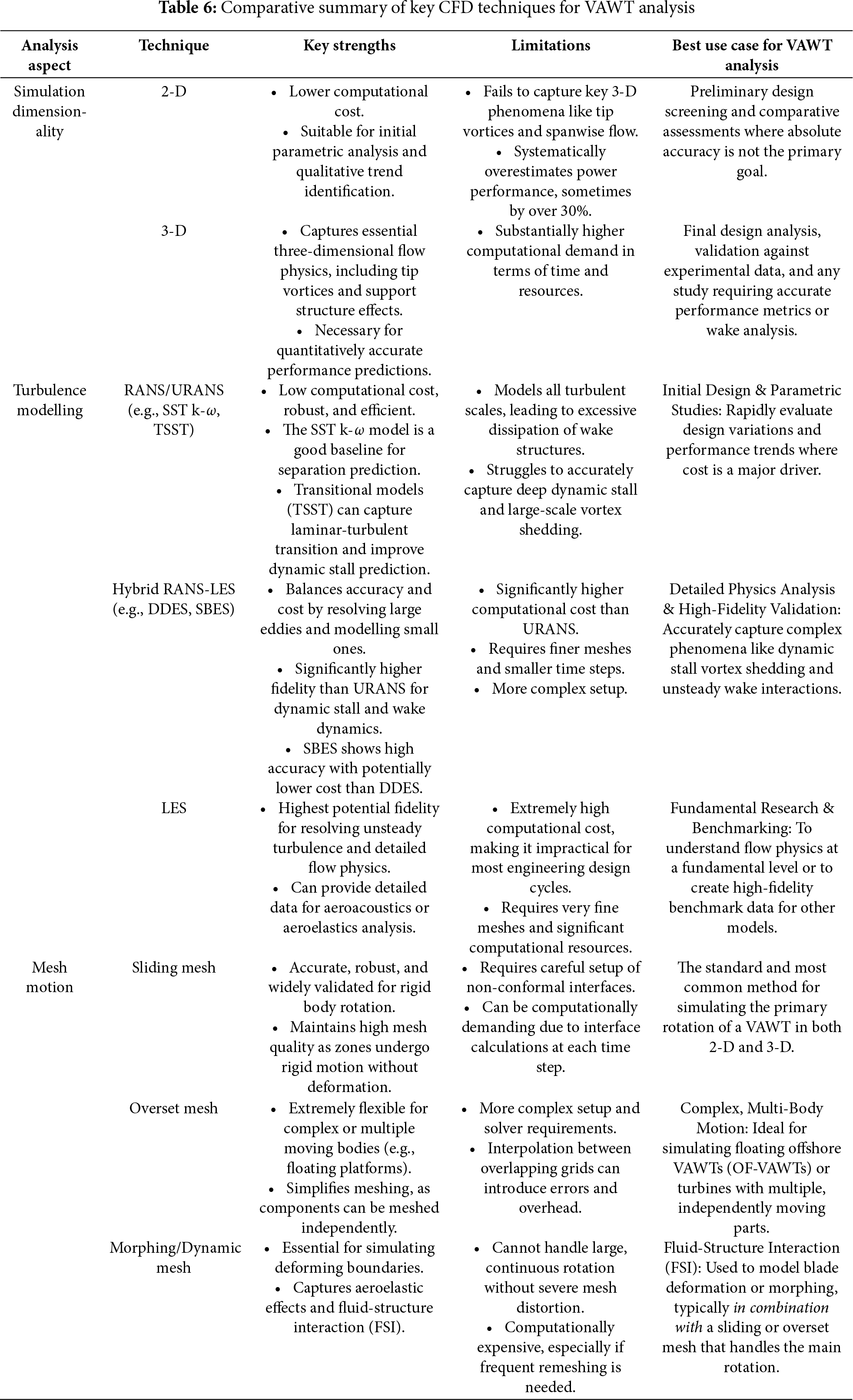
The selection of an appropriate CFD methodology for VAWT analysis involves a series of critical decisions, each with a trade-off between computational cost, setup complexity, and physical fidelity. Table 6 provides a consolidated overview of the primary techniques discussed in this review, comparing their relative advantages, disadvantages, and most suitable applications for VAWT research and development.

4  Predicting and Analysing VAWT Aerodynamic Performance via CFD

A primary application of CFD in VAWT research is the prediction and detailed analysis of aerodynamic performance under various conditions. CFD simulations provide access to key metrics characterising the turbine’s efficiency and loading.

4.1 Key Performance Metrics–Important Parameters for VAWT Analysis in CFD

CFD solvers calculate the forces and moments acting on the turbine blades by integrating the pressure and viscous shear stress distributions over the blade surfaces [163]. From these fundamental quantities, several critical performance metrics are derived:

•   Torque (T): The rotational moment generated by the aerodynamic forces on the blades around the turbine’s axis of rotation. Due to the constantly changing AoA and phenomena like dynamic stall, the instantaneous torque produced by a VAWT blade varies significantly throughout each revolution [42]. CFD calculates both the instantaneous torque and, by averaging over one or more full cycles (after reaching a periodic state), the mean torque, which is essential for power calculation [68]. Torque is often non-dimensionalised into a Torque Coefficient (Ct or Cm) using reference parameters: Ct=T/(0.5×ρ×A×R×V∞2), where ρ is air density, A is a reference area (typically rotor swept area D×H), R is the rotor radius, and V∞2 is the freestream wind speed [80]. Note that Cm is sometimes used interchangeably or to denote a moment coefficient based on chord length [68].

•   Power (P): The rate at which the turbine extracts kinetic energy from the wind and converts it into mechanical rotational energy. It is calculated directly from the mean torque (Tavg) and the rotational speed (ω, in radians per second): P=Tavg×ω [80]. Additionally, the primary measure of aerodynamic efficiency is the power coefficient (Cp), defined as the ratio of the extracted power to the total power available in the wind passing through the rotor’s swept area: Cp=P/(0.5×ρ×A×V∞3) [80]. Cp is related to the torque coefficient by Cp=Ct×λ, where λ is the Tip Speed Ratio [80]. CP is the most common metric used to compare the performance of different wind turbine designs [41].

•   Aerodynamic Forces: CFD calculates the fundamental aerodynamic forces acting on the blades. These can be resolved into components parallel and perpendicular to the relative wind (Lift, Cl, and Drag, Cd) or components normal and tangential to the blade chord (Normal Force, Fn, and Tangential Force, Ft) [42]. The tangential force component is directly responsible for generating torque [56]. These forces are also non-dimensionalised into various coefficients (Cl, Cd, Cn, Ct_force) using the dynamic pressure of the relative wind and a reference area (usually blade chord times span) [164].

•   Tip Speed Ratio (TSR or λ): This dimensionless parameter relates the speed of the blade tips (ωR) to the freestream wind speed (V∞): λ=ωR/V∞. Plotting performance metrics like Cp and Ct as a function of TSR (i.e., generating Cp−λ and Ct−λ curves) is the standard way to characterise a VAWT’s aerodynamic performance across its operating range [53].

The ability of CFD to provide not just average performance metrics like Cp, but also the instantaneous variation of forces and torque throughout a rotation cycle, is a significant advantage [42]. This time-resolved data is invaluable for understanding the underlying physics responsible for performance characteristics. For example, plotting instantaneous torque vs. azimuthal angle can clearly show the detrimental impact of dynamic stall (manifesting as sharp drops or negative torque contributions) or the effects of blade-wake interactions [83]. Furthermore, these instantaneous load fluctuations are critical inputs for structural analysis and fatigue life assessment, aspects that cannot be evaluated using average performance values alone.

4.2 Parametric Analysis—What Can Be Expected from the Obtained CFD Data

CFD enables the virtual testing of numerous geometric modifications, such as solidity, which is the ratio of blade area to the rotor’s swept area. CFD-based parametric studies show that increasing solidity generally increases the maximum power coefficient but shifts the optimal performance to a lower TSR. For example, one study found that increasing the rotor solidity from 0.24 to 0.48 increased the peak Cp by approximately 15%, but the TSR at which this peak occurred dropped from 3.1 to 2.5 [60]. This type of analysis is critical for tuning a turbine’s design to match the expected wind conditions of a specific site.

•   Effect of Tip Speed Ratio (TSR): By running simulations at various rotational speeds (Ω) for a given wind speed (V∞), CFD generates the fundamental Cp−λ and Ct−λ curves [53]. These curves reveal the optimal TSR at which the turbine achieves maximum efficiency (peak Cp) and map the performance across the operational range [56]. They also clearly illustrate the performance degradation at low TSRs due to effects like dynamic stall [42].

•   Effect of Wind Conditions: CFD allows analysis under varying freestream wind speeds (V∞) and can incorporate realistic atmospheric conditions, such as specific turbulence intensity levels, turbulent length scales, or skewed inflow profiles characteristic of urban or complex terrain environments [44]. This helps predict performance in real-world deployment scenarios.

•   Effect of Design Parameters: CFD enables the virtual testing of numerous geometric modifications:

Solidity: Investigating the impact of changing the number of blades (N) or the blade chord length (c) relative to the diameter (D) [162].

Blade Pitch Angle: Assessing the effect of fixed pitch angles or evaluating the potential benefits of complex variable pitch schedules.

Airfoil Profile: Comparing the performance of different standard airfoil shapes (e.g., NACA series) or evaluating novel, custom-designed profiles [36].

Aspect Ratio (Height/Diameter): Studying its influence on performance and flow structures [67].

Other Geometric Features: Analysing the impact of support strut design, tower presence, blade endplates, or helical twist [56].

The performance of a VAWT is sensitive to a complex interplay of these parameters. For example, the optimal TSR often changes with solidity, and the effectiveness of a particular airfoil shape can depend on the Reynolds number and TSR range [53]. Exploring this multi-dimensional design space experimentally would be highly costly and time-consuming [165]. CFD provides a uniquely powerful and cost-effective means to perform these extensive parametric sweeps, identify key sensitivities, and guide the design towards optimal configurations for specific applications [162].

4.2.1 Performance Enhancement via Blade Modifications: Some Case Studies of CFD Application

A primary application of CFD in VAWT development is to investigate and optimize blade modifications designed to improve aerodynamic performance by addressing issues like poor self-starting and dynamic stall. As categorized by recent reviews, these solutions can be broadly classified as either passive or active techniques.

•   Passive techniques involve geometric modifications that do not require external energy. They alter the flow based on their fixed shape and include features like slats, winglets, dimples, and leading-edge serrations [97,111,166].

•   Active techniques require external energy and control systems to dynamically manipulate the flow. Examples include variable-pitch systems, morphing blades, and plasma actuators [112,167,168].

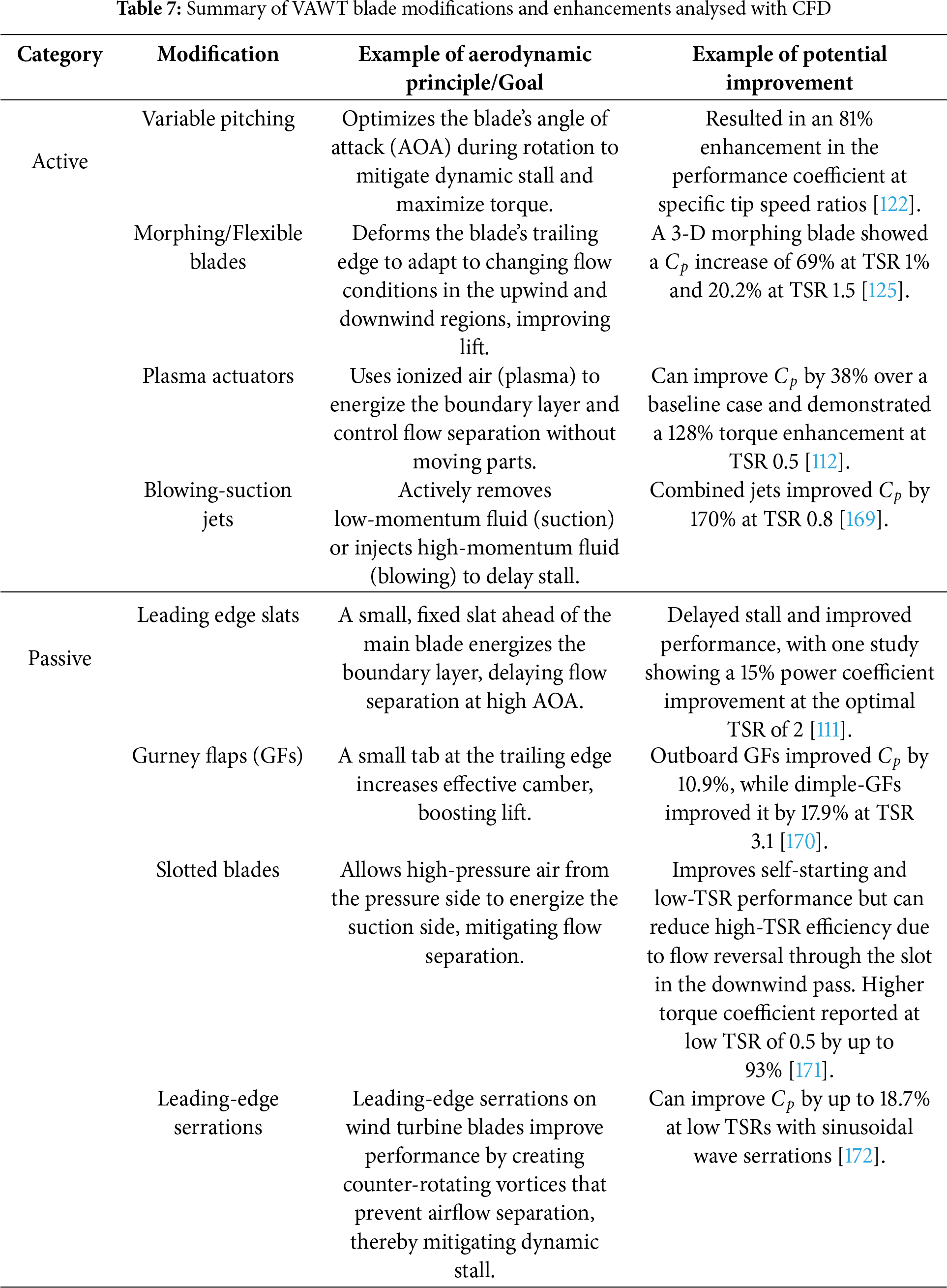
CFD is instrumental in quantifying the effectiveness of both types of modifications. Table 7 provides a summary of various advancements, categorized as active or passive, and highlights their principles and reported outcomes from numerical and experimental studies.

As the findings in Table 7 indicate (coupled with the discussions found in Section 3 and Table 1), there is often a trade-off between performance and practicality. Active solutions like variable pitching and morphing blades the highest potential performance gains by adapting to the flow, but at the cost of increased complexity, maintenance, and system cost. Passive solutions are simpler and more robust, but their benefits are often confined to specific operating ranges, sometimes leading to performance penalties at off-design conditions. The ongoing challenge, which CFD is uniquely suited to address, is the development of solutions that bridge this gap, offering significant aerodynamic improvement without compromising practical viability. For additional work on blade modifications—beyond CFD-focused studies—see [41].

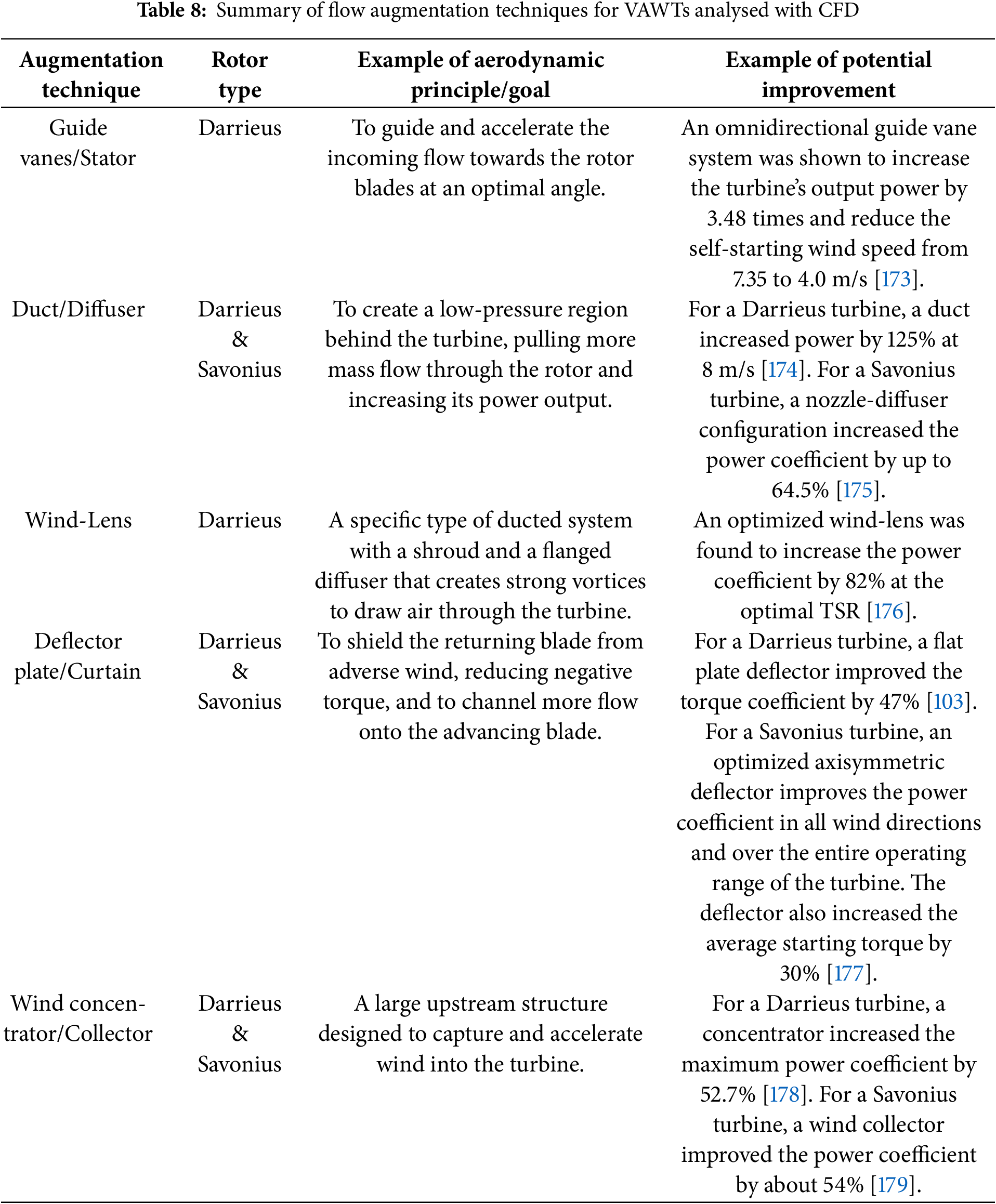
4.2.2 Performance Enhancement via Flow Augmentation Systems: Some Case Studies of CFD Application

Beyond modifying the turbine blades themselves, a significant area of VAWT research involves using external structures to augment the flow entering the rotor. These flow augmentation techniques aim to increase the local wind velocity, guide the flow onto the blades at more favorable angles, and shield the returning blades from negative torque. Because these systems create complex aerodynamic interactions between the stationary structure and the rotating turbine, CFD is the primary tool for their design and analysis.

CFD simulations are essential for modelling the flow acceleration through ducts or nozzles, the pressure changes induced by diffusers, and the shielding effects of deflectors. Such analyses allow for the optimization of the augmentation device’s geometry and its placement relative to the rotor to maximize power output. Table 8 summarizes several common flow augmentation techniques for both Darrieus and Savonius rotors that have been evaluated using CFD.

4.3 Post-Processing for Performance Evaluation

Once a CFD simulation has converged and run for a sufficient number of cycles, specialised post-processing tools within the CFD software are used to extract and analyse the performance data [80].

•   Calculating Forces and Torque: The solver directly computes the net forces (e.g., lift, drag) and moments (torque) acting on specified surfaces (like the turbine blades) by integrating the pressure and viscous shear stress distributions over the mesh faces defining those surfaces [163]. The underlying calculation involves summing the contributions from each face element, considering both pressure forces (pressure * area * moment arm) and viscous forces (shear stress * area * moment arm) [163].

•   Calculating Coefficients: To obtain non-dimensional coefficients like Cp and Ct, the computed forces and torques must be divided by appropriate reference quantities involving fluid density (ρ), a reference area (A), a reference length (like rotor radius R or chord c), and the freestream velocity (V∞) or relative velocity [80]. It is imperative that the definitions used for these reference parameters (especially the reference area A, e.g., rotor swept area DH vs. blade planform area Nc * H) are clearly stated and consistently applied, as inconsistencies can lead to misleading comparisons between different studies or simulations.

•   Averaging: For unsteady (URANS or SRS) simulations, the instantaneous torque and power values fluctuate over a rotation cycle. To obtain the mean performance metrics (average Cp, average Ct) representative of the turbine’s overall output, these instantaneous values must be averaged over one or more complete revolutions after the simulation has reached a statistically steady, periodic state [68].

•   Validation: A critical step in post-processing is comparing the CFD-predicted performance characteristics (e.g., the Cp−λ curve) against available experimental data from wind tunnel tests or field measurements [83]. Good agreement provides confidence in the simulation setup and results, while significant discrepancies may indicate issues with the CFD model (e.g., mesh, turbulence model) or the experimental data.

4.4 CFD Analysis of Self-Starting Capability of VAWTs

A significant historical and ongoing challenge for Darrieus-type VAWTs is their inherently poor self-starting capability. At low rotational speeds (or from a standstill), the blades experience very high angles of attack, leading to massive flow separation and dynamic stall. This often produces negative torque over parts of the rotation, preventing the turbine from accelerating on its own. CFD is an indispensable tool for diagnosing the root causes of this issue and for evaluating the effectiveness of strategies designed to overcome it [41,180,181].

4.4.1 Diagnosing Starting Problems with CFD: Performance Curves and Flow Visualisation

To understand the self-starting problem, a combination of quantitative performance curves and detailed flow visualization is required. A static CFD analysis can generate a static torque coefficient (CTS, or Cts, or Cms) vs. azimuthal angle curve (examples are as shown in Fig. 14a,b). The static torque performance of a VAWT refers to the amount of torque produced by the rotor when it is stationary and wind is blowing. In CFD, to obtain the static torque of the rotor, one could run a numerical simulation at steady state (i.e., rotor is fixed) at different rotor azimuthal positions. A turbine is considered to have starting potential only if the average static torque is positive, allowing it to overcome initial bearing friction and begin to turn. This method is helpful for a preliminary assessment. For instance, Uma Reddy et al. [182] used static torque curves to show that adding auxiliary blades increased the maximum static torque by 84%, indicating a significantly stronger initial turning force.

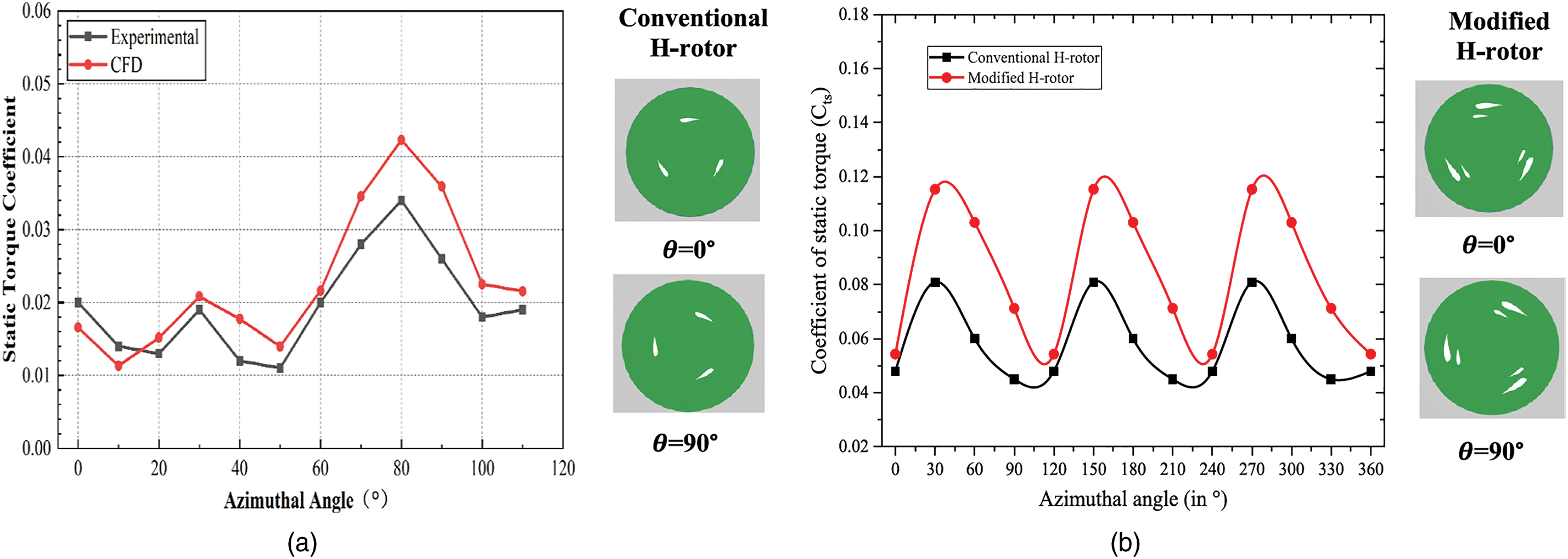
Figure 14: Illustrating the relationship between the static torque coefficient and the azimuthal angle. In general, the higher the static torque coefficient, the better the self-start characteristic of the rotor is. Figures are obtained from studies of (a) Xu et al. [180] and (b) Uma Reddy et al. [182]

While a high static torque coefficient is necessary for initial rotation, studies show it is not a sufficient predictor of dynamic self-starting success. A key finding, demonstrated by Xu et al. [180], is that a high initial static torque does not guarantee a successful or fast start-up. Their study showed that a turbine starting at an angle with maximum static torque took longer to accelerate through the initial phase than one starting from an angle with minimum static torque. This is because the static analysis cannot capture the complex, unsteady aerodynamic effects that occur once the rotor begins to move, particularly as it enters the low-TSR “dead band” or “plateau state” where dynamic stall and blade-wake interactions can generate significant negative torque and stall the acceleration. Furthermore, reference [180] shows that a dynamic start-up analysis via TSR vs. time curve, which visualises the entire journey of the turbine from rest (TSR = 0) to its final operational speed, would be a better choice of analysis tool. This curve clearly reveals the initial rotation (which is often a slow rotation), the critical plateau state (or “dead band”, where acceleration may stagnate), and whether the turbine successfully accelerates to its final operating speed (i.e., lift acceleration state towards stable operating TSR, where the aerodynamic torque balances any resistive loads). For example, to better showcase the self-starting characteristics of a VAWT rotor, Fig. 15 was developed by [180] based on the insights into the self-starting characteristics of VAWT rotors from [183,184]. Worasinchai et al. [183] divide the self-starting process into a “combined state” and a “full lift-driven state”. The “full lift-driven state” is further divided into two thrust generation states: “discrete” and “continuous”. They considered reaching the “continuous thrust-producing state” to be the completion of the self-starting process, as indicated by the red dot in the figure. In a similar study, Hill et al. [184] divided the self-starting process into four states: a “linear regime”, a “plateau” state, a “lift” state, and an “equilibrium” state. Celik et al. [185] came to a similar conclusion to [184], in which they considered the wind turbine reaching a stable condition as the completion of the self-starting process, as indicated by the green dot in Fig. 15. The Lunt point (i.e., blue dot) refers to the conclusion made by Lunt [186] in which they adopted a TSR of 1 as the self-starting point.

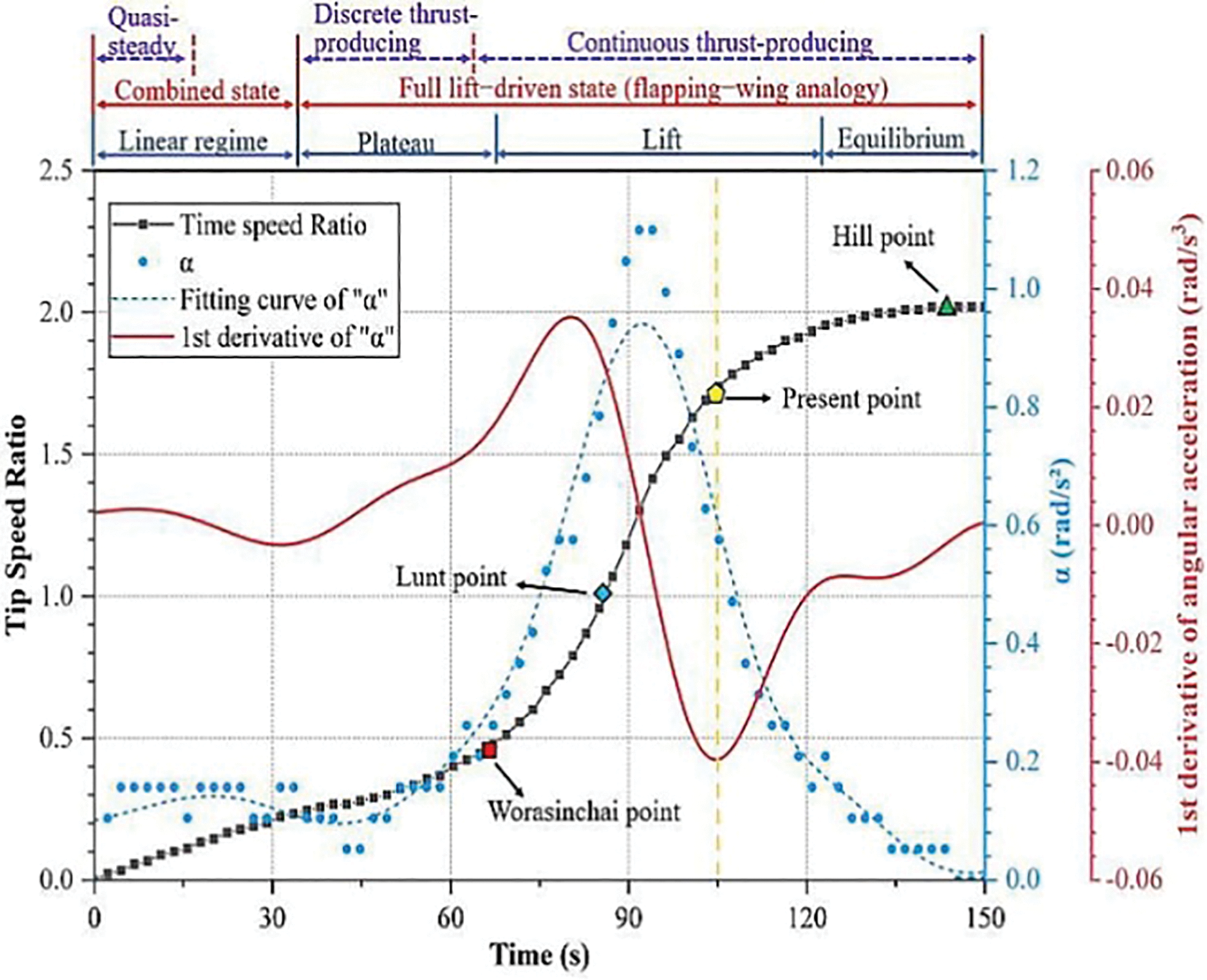
Figure 15: A self-starting process of a NACA2418 VAWT [180]

CFD contour plots are essential for visualising the underlying physics that performance curves cannot show alone. They allow researchers to diagnose the precise causes of poor torque generation. (Note: General discussions of different visualisation tools are discussed in Section 5).

•   Vorticity Contours: These are used to track the evolution of the flow from a complex, separated state to an organised one. For example, Celik et al. [185] used vorticity contours to demonstrate that during the initial start-up phase (TSR < 1), the flow is characterised by large, complex vortices and separated flow. As the turbine successfully accelerates to its operational speed, the same contours indicate that the blade vortices become smaller, more organised, and the flow becomes more attached, which is essential for generating the higher lift force required for efficient operation.

•   Pressure Contours: These plots diagnose the sources of positive and negative torque at specific blade positions. Xu et al. [180] used static pressure contours to analyse why a turbine failed to start at 5.5 m/s but succeeded at 6 m/s. The contours revealed that at lower wind speeds, the pressure distribution on the blades at azimuthal angles between 60° and 120° generated a significant negative torque that offset any positive torque gained elsewhere. This level of detailed, localised diagnostic information is only possible through CFD.

•   Streamline Plots: Streamlines are highly effective for visualising flow separation and the efficacy of flow control devices. For instance, Uma Reddy et al. [182] used streamline plots to compare a conventional H-rotor with one modified with auxiliary blades. The visualisations clearly showed significant flow separation near the trailing edge of the conventional blade. In contrast, for the modified rotor, the streamlines remained “more attached to the surface of the main blade”. This directly illustrates the physical mechanism by which the auxiliary blades improve performance.

4.4.2 Aerodynamic Factors and Improvement Strategies

While Darrieus turbines are lift-driven at operational speeds, CFD analysis has revealed that in the critical start-up region (TSR < 1), the drag force can have a significant positive contribution to the overall torque. Numerous strategies, both passive and active, leverage CFD for their design and aim to optimise the torque profile at low TSRs. Some examples are discussed below:

•   Passive Flow Control Devices: The effect of modifying blade surfaces to enhance VAWT performance has been explored through various design strategies. One such approach involves adding cavities to the blade surface, as demonstrated by Yousefi Roshan et al. [187], who used CFD to show that strategically placed cavities can trap vortices and significantly boost performance. A single cavity located on the upper surface near the trailing edge was found to increase the static torque coefficient by 5 to 7 times compared to a smooth blade at certain angles, greatly improving the self-starting potential. Another strategy involves the addition of fixed auxiliary blades positioned ahead of the main blades. In this approach, Uma Reddy et al. [182] showed that the auxiliary blades act as passive flow control devices, reducing separation on the main blade. Their experimental and numerical results indicated that this configuration enhanced the maximum static torque coefficient by 84% compared to a conventional H-rotor.

•   Blade and Rotor Modifications: The selection of airfoil type and pitch angle plays a crucial role in determining a VAWT’s self-starting capability. CFD simulations have shown that cambered airfoils, such as the NACA2418, outperform symmetric profiles like the NACA0018 in terms of starting performance. In particular, Xu et al. [180] demonstrated that increasing the pitch angle of a NACA2418 blade to 10° reduced its start-up time by 20% compared to a 0° pitch angle. Another innovative design involves the use of J-shaped blades, which feature a concave profile to harness drag more effectively and generate a stronger starting torque. Farzadi and Bazargan [188], using 3-D CFD analysis, found that at a wind speed of 5 m/s, J-type blades increased the average self-starting torque by 37.6% compared to traditional straight blades, highlighting their potential for use in low-wind environments.

•   Turbine Pair and Farm Optimisation: The self-starting of a VAWT is further complicated when it is part of an array. Fatahian et al. [181] used a CFD-Taguchi optimisation method to study the start-up of VAWT pairs. They found that the angle between adjacent rotors was the most significant factor affecting start-up and that a downstream rotor in an optimised layout could benefit from the wake of the upstream rotor, starting faster and at a lower TSR.

4.5 Advanced CFD Optimisation Using Design of Experiments (DoE) and Surrogate Models

While traditional parametric studies are helpful, they can be computationally prohibitive for exploring designs with many variables. Modern VAWT optimisation overcomes this challenge by coupling CFD with Design of Experiments (DoE) methodologies. DoE provides a statistical framework for intelligently selecting a small, representative set of CFD simulations to run. The data from these runs is then used to create a “surrogate model” (or metamodel) that approximates the whole performance landscape, allowing for efficient optimisation without the cost of a brute-force CFD approach. Key techniques prominent in recent VAWT research include:

•   Taguchi Method: This robust DoE approach uses orthogonal arrays to drastically reduce the number of required simulations, making it highly efficient for screening a large number of design parameters. In other words, it is highly effective for sensitivity analysis, determining which design parameters have the most significant impact on performance. Recent studies have demonstrated the effectiveness of the DoE and Taguchi approaches in optimising blade geometry, pitch, overlap ratio, and other key variables, leading to significant improvements in power coefficients (with reported increases of up to 22.8% to 177%) and self-starting capabilities [181,189,190]. For instance, Fatahian et al. [181] employed a CFD-Taguchi approach combined with Analysis of Variance (ANOVA) to optimise the layout of VAWT pairs. The methodology enabled them not only to find an optimal configuration but also to quantify the impact of each parameter. They concluded that the angle between adjacent rotors was the most critical factor, accounting for 55.3% of the variation in start-up time. The Taguchi method has also been proven to enhance computational efficiency. Peng et al. [191] used the Taguchi method to optimise the layout of twin VAWTs. By using an L16 orthogonal array, they were able to investigate 5 different parameters at 4 levels each on the twin-VAWT power output, reducing the number of required high-fidelity CFD simulations from a potential 1024 to just 16. Additionally, the method has proven versatile, being applied not only to Darrieus turbines but also to hydrokinetic turbines, as shown by Al-Gburi et al. [189] and for design and optimisation of VAWT airfoil blades in a study by Cheng et al. [192]. However, such methods cannot quantificationally provide predictions (i.e., the response) for other input combinations, therefore they were often used to diagnose the most influential parameters or offer more reasonable searching domains for additional optimization approaches [193]. The comparative studies suggest that DoE and Taguchi methods offer a good balance between efficiency and accuracy, though hybrid approaches (e.g., combining DoE with genetic algorithms or adjoint methods) may yield further improvements.

•   Response Surface Methodology (RSM): RSM uses the results from a planned set of CFD simulations to fit a polynomial equation, creating a “response surface”. This surface acts as a fast surrogate that maps design inputs (e.g., blade solidity, pitch angle, chord length, solidity, airfoil shape) to a performance output (e.g., Cp). The optimal design can then be found mathematically from this surface, as demonstrated in various turbine optimization studies, in which improvements in power coefficient (up to 70% in some cases) and torque have been reported [181,194–196] Studies based on RSM have shown that slotted and morphing blades, as well as the addition of flow control features like boundary layer suction slots, can further enhance aerodynamic performance [125,195,197,198]. Sensitivity analyses using RSM and methods like Morris’ method or ANOVA have identified the most influential design variables, with pitch angle, chord length, and solidity often having the greatest impact on performance [196,197,199,200]. These analyses enable targeted optimization and reduce the dimensionality of the design space, making high-fidelity simulations more tractable.

•   Kriging Surrogate Models: Kriging has become a particularly powerful technique for VAWT optimization due to its high accuracy with small sample sizes. It is a geostatistical interpolation method that provides not only a prediction but also an estimate of the prediction’s uncertainty. Additionally, Kriging is widely used to build accurate surrogate models for VAWT performance, enabling rapid optimization and sensitivity analysis with reduced CFD runs [201–203]. Kriging-based models can achieve high prediction accuracy (R² > 0.98) and are often more stable and efficient than artificial neural network (ANN)-based surrogates [203]. Studies employ variance-based methods (e.g., ANOVA, Morris method, Sobol indices) to quantify the impact of each design variable on performance outcomes. Pitch angle and tip speed ratio consistently emerge as the most critical parameters for aerodynamic performance, while structural parameters (e.g., blade thickness, material layup) are crucial for reliability and fatigue life [196,199,202,204]. As demonstrated by Wang & Zhang [205], the typical optimisation workflow involves parameterizing the airfoil geometry using a method like the Classification and Shape Transformation (CST) function, generating a limited number of sample designs across the design space using Latin Hypercube Sampling (LHS), running high-fidelity CFD simulations for these sample points to build a training dataset, and lastly, constructing a high-precision Kriging model, which is then validated [205] achieved a coefficient of determination (R2) of 0.91368, indicating excellent accuracy. Similarly, [205] found that Kriging models for twin-VAWTs reached R2 values over 0.98. Furthermore, this method allows for coupling with an efficient optimisation algorithm, such as a Multi-Island Genetic Algorithm (MIGA), to search for the global optimum.

By integrating these DoE and surrogate modelling techniques, researchers can leverage the detailed physics from CFD to conduct sophisticated multi-parameter optimizations that would otherwise be computationally impossible.

5  Visualising and Understanding the Flow Field around VAWT Using CFD

Beyond predicting overall performance metrics, one of the most significant contributions of CFD to VAWT analysis is its ability to provide detailed visualisations of the complex flow field surrounding the turbine. These visualisations offer invaluable insights into the underlying aerodynamic phenomena that govern turbine behaviour, often revealing details inaccessible through experimental measurements alone. The following subsections discuss the many visualisation tools that can help researchers further understand what is happening to the vertical axis wind rotor.

5.1 Flow Pattern Visualisation

The flow pattern visualisation is used to illustrate the general flow patterns in and around vertical axis wind turbines. The standard post-processing techniques include:

•   Streamlines (e.g., Fig. 16a): Lines that are instantaneously tangent to the velocity vector, illustrating the path fluid particles would take. Streamlines can clearly show areas of flow attachment, separation, recirculation zones (e.g., behind the shaft or stalled blades), and the overall deflection of the flow by the turbine [206].

•   Velocity Vectors (e.g., Fig. 16b): Arrows indicating the direction and magnitude of velocity at various points in the domain. Vector plots provide a direct view of the flow field, highlighting regions of high and low velocity and flow direction changes around the blades and in the wake.

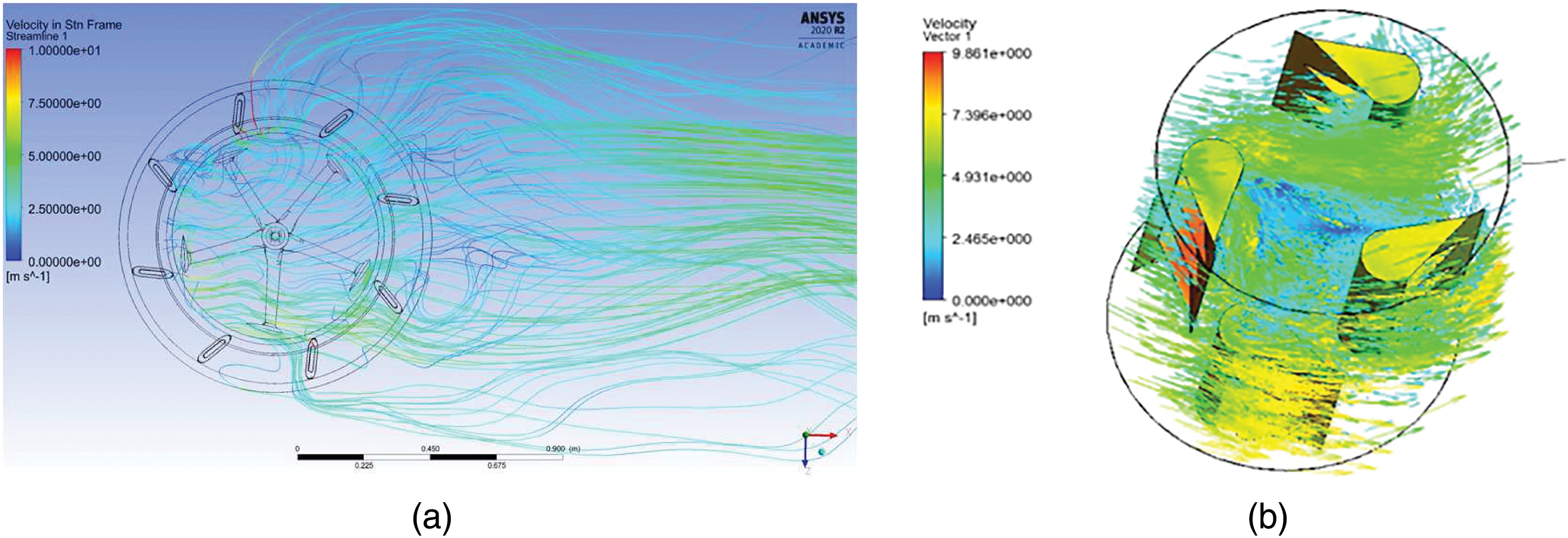
Figure 16: Examples of (a) streamline plot [207], and (b) velocity vector plot [208]

5.2 Pressure and Velocity Field Analysis

Quantitative information about the flow field is often presented using contour plots:

•   Pressure Contours (e.g., Fig. 17a): Display the distribution of static or total pressure on the blade surfaces and in the surrounding fluid [206]. High pressure on the windward side and low pressure on the leeward (suction) side of an airfoil generate lift. Visualising pressure distributions helps understand how forces are generated at different points in the rotation cycle and identify pressure gradients driving the flow [44].

•   Velocity Contours (e.g., Fig. 17b): Show the spatial variation of flow speed [83]. These plots depict flow acceleration over the suction surfaces of the blades, regions of low velocity associated with flow separation or stall, and the characteristic velocity deficit in the turbine’s wake.

Figure 17: Examples of (a) pressure contour plot [83], and (b) velocity contour plot [209]

5.3 Analysis of Vortex Dynamics and Dynamic Stall

CFD particularly excels at capturing and visualising the complex vortical structures inherent to VAWT operation:

•   Vorticity Contours/Magnitude (e.g., Fig. 18): Vorticity is a measure of local fluid rotation. Contour plots of vorticity magnitude highlight regions where the fluid is swirling, effectively identifying shed vortices from blade leading edges (during dynamic stall), trailing edges, and blade tips (in 3-D simulations) [42]. Analysing the strength, location, and convection of these vortices is crucial for understanding unsteady loads, energy losses, and wake behaviour [64].

Figure 18: Example of vorticity contours on VAWT blades [210]

•   Dynamic Stall Visualisation (e.g., Fig. 19): CFD allows for a detailed, time-resolved visualisation of the entire dynamic stall process [42], which would be very beneficial in understanding the complex and chaotic wake-blade interaction. CFD simulations can show:

The initial boundary layer separation often starts near the trailing edge and progresses forward as AoA increases.

○   The formation of a Laminar Separation Bubble (LSB) near the leading edge and its potential bursting.

○   The roll-up of the shear layer into the distinct Dynamic Stall Vortex (DSV) near the leading edge.

○   The convection of the DSV across the airfoil’s suction surface.

○   The eventual shedding of the DSV (and potentially secondary or trailing edge vortices) into the wake. The timing, size, and trajectory of these vortical structures, which depend strongly on TSR and Reynolds number, can be meticulously tracked in CFD visualisations [42,56,206].

Vortex Identification Criteria (3-D) (e.g., Fig. 20): In three-dimensional simulations, scalar criteria like the Q-criterion or Lambda2 are often used to generate iso-surfaces that identify and visualise coherent vortical structures (like tip vortices or complex wake eddies) more clearly than simple vorticity magnitude plots [71,206].

Figure 19: Example of dynamic stall visualisation, with LSB and separation of flows [211]

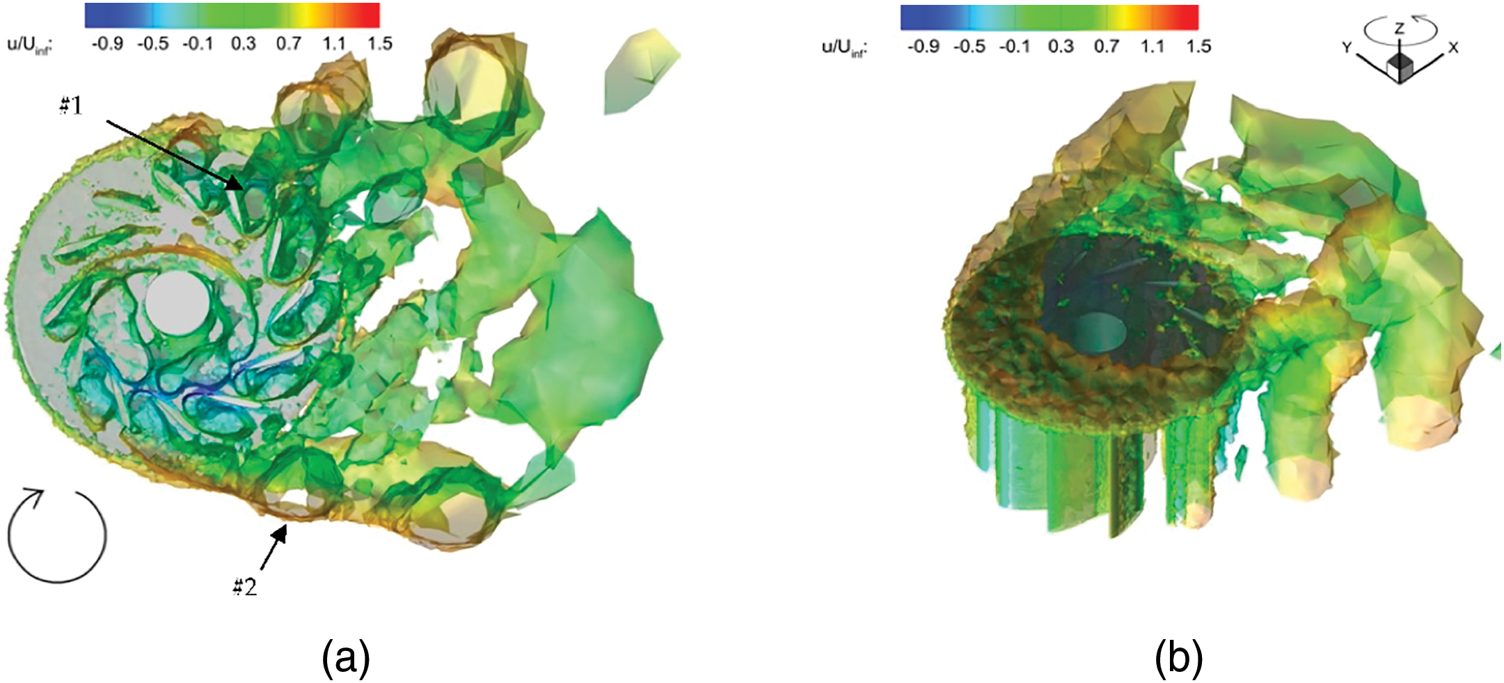
Figure 20: Example of Q-criterion representation of eddies on VAWT’s (a) bottom view, and (b) isometric view [83]

5.4 Wake Structure Characterisation

CFD is used to quantify the wake recovery distance, a key parameter for wind farm spacing, as listed below. While HAWT wakes can persist for over 10 rotor diameters (D), VAWT wakes tend to recover faster due to enhanced mixing from large-scale turbulence structures. CFD studies often show VAWT wake velocity deficits recovering to less than 5% of the freestream value within [74,107] 6 to 9 rotor diameters. This is a critical advantage for densely packed wind farms [212].

•   Wake Visualisation: Plots of velocity deficit (difference from freestream velocity), turbulence intensity, or vorticity contours in cross-sections downstream of the turbine reveal the wake’s size, shape, intensity, and how it evolves with distance [35,40,42,83].

•   Wake Asymmetry and Convection: VAWT wakes are often asymmetric due to the differing aerodynamic experiences of the blades in the upwind vs. downwind passes, particularly when dynamic stall occurs [19]. In skewed inflow conditions, the wake convects downstream at an oblique angle [162,213]. CFD captures these effects.

•   Vortex Interaction in Wake: Visualisations can track the convection and interaction of vortices shed from the blades (DSV, trailing edge, tip vortices) as they move downstream within the wake [19,40,42,83]. These interactions significantly influence the wake’s turbulence characteristics and recovery rate, which is critical for predicting the performance of downstream turbines in a wind farm.

•   Wake Recovery: CFD simulations can predict the downstream distance required for the velocity deficit in the wake to recover towards the freestream value [19,35,83]. Studies often quantify this distance to help future researchers best understand the effect of vertical blades in the downstream region of the rotor (e.g., wake recovery observed around 9 turbine diameters downstream in [83]). VAWT wakes are generally observed to recover more quickly than HAWT wakes, a phenomenon potentially linked to the enhanced mixing induced by strong tip vortices and large-scale wake structures [65].

The powerful visualisation capabilities of CFD transform it from a mere performance prediction tool into a crucial diagnostic instrument. By allowing engineers and researchers to “see” intricate and transient flow phenomena like the birth and shedding of a dynamic stall vortex or the complex interactions within the turbine wake, CFD provides a depth of understanding that is often unattainable through experiments or analytical models alone [71,77]. This visual insight is key to diagnosing the root causes of performance limitations or detrimental structural loads.

Furthermore, CFD bridges the gap between microscopic flow details and macroscopic outcomes. It allows researchers to connect local phenomena, such as the state of the boundary layer on a small section of the blade, the pressure within a vortex core, or the local rate of vorticity generation, directly to global performance metrics like Cp and Ct, or to overall structural loads [64,163]. This ability to link scales is fundamental for developing a causal understanding of how subtle changes in flow physics translate into overall turbine behaviour, which in turn guides effective optimisation strategies.

It is also important to note the distinction between 2-D and 3-D visualisations. While 2-D CFD can effectively visualise spanwise-averaged or mid-span structures like the primary dynamic stall vortex, it inherently misses three-dimensional effects such as tip vortices, spanwise flow variations, and the complex breakdown of vortices in the wake [19,64,71]. 3-D visualisations, often employing techniques like Q-criterion iso-surfaces, reveal a significantly more intricate vortical structure and wake evolution [19,206]. Relying solely on 2-D visualisations can therefore provide an incomplete or potentially misleading picture of the full flow physics, reinforcing the need for 3-D simulations for comprehensive understanding, particularly of wake dynamics and recovery mechanisms, despite the associated increase in computational cost [71].

6  Comparing CFD Analysis with Other Methods

While CFD is a powerful tool for VAWT analysis, it exists alongside other established methods, namely physical wind tunnel experiments and lower-fidelity analytical or semi-empirical models. Understanding each approach’s relative strengths and weaknesses is crucial for selecting the appropriate tool(s) for a given task in the research and development process.

6.1 CFD Model Validation Against Experimental Data

The validation of computational fluid dynamics (CFD) models for Savonius and Darrieus vertical axis wind turbines (VAWTs) is a critical step in ensuring the reliability of numerical predictions for turbine performance and flow physics. Both 2-D and 3-D CFD approaches are widely used, with each offering distinct advantages and limitations. For Savonius turbines, 2-D models are often employed due to their simpler geometry and lower computational cost, but 3-D models are increasingly used to capture complex flow phenomena such as tip vortices and three-dimensional wake effects [118,214–216]. Darrieus turbines, with their lift-based operation and more intricate blade interactions, often require 3-D modelling for accurate prediction, especially at higher tip speed ratios and for capturing dynamic stall and blade-vortex interactions [40,217–220]. Validation is typically performed by comparing CFD results—such as the power coefficient (Cp) vs. tip speed ratio (TSR), torque, and flow fields—against experimental data obtained from wind tunnel tests, theoretical models, or field measurements [221,222]. Fig. 21 presents examples of these comparisons. As discussed extensively throughout the article, the choice of turbulence model, mesh resolution, and boundary conditions are key factors influencing the accuracy of CFD predictions. Sensitivity analyses are often conducted to ensure robustness. Overall, the literature demonstrates a trend toward more sophisticated 3-D simulations and multi-physics validation strategies, but also highlights ongoing challenges in bridging the gap between numerical and experimental results, particularly for complex hybrid and urban VAWT applications.

Figure 21: Examples of CFD validation for various VAWT types and CFD models. (a) URANS CFD validations for 2-D and 3-D Darrieus CFD models [223], (b) comparison of Darrieus power coefficient vs. TSR between 3-D DMST, 3-D CFD and experimental data [217], and (c) validation of Savonius rotor using different turbulence models with experimental data [214]

2-D CFD models are commonly used for initial validation of Savonius turbines due to their drag-based, symmetric geometry, and for Darrieus turbines at low computational cost. However, a consistent finding across the literature is that 2-D CFD simulations systematically over-predict the performance of Darrieus turbines. While 2-D models are computationally cheaper and practical for preliminary analysis, their results often exhibit significant quantitative disparities when compared to experimental data. 2-D models often fail to capture three-dimensional effects such as tip losses, secondary flows, and complex wake structures, which are significant in Darrieus turbines and at higher tip speed ratios. 3-D CFD models, while computationally intensive and requiring careful experimental design, provide more accurate predictions of performance metrics (Cp, torque) and flow features, especially for Darrieus and hybrid turbines.

As previously discussed, significant challenges in CFD validation include selecting the appropriate turbulence model (e.g., RANS, SST k-ω, LES), mesh sensitivity, and accurately representing boundary conditions. Discrepancies between CFD and experiments are often within 5%–15% for well-validated models but can be higher for complex or novel configurations [220,221,223]. The primary sources for the discrepancies often found in CFD models are:

•   Neglect of 3-D aerodynamic effects: 2-D simulations are fundamentally unable to capture three-dimensional flow phenomena that cause significant power loss. This includes the formation of blade tip vortices and spanwise flow along the blade, which are substantial sources of induced drag and are not present in a 2-D plane.

•   Absence of parasitic drag: The 2-D model does not account for the drag produced by physical components like the rotor’s central shaft, support arms, and connection points. This parasitic drag consumes a portion of the generated torque in a real-world turbine, resulting in overly optimistic performance predictions in the simulation.

•   Unaccounted experimental losses: Experimental test rigs have inherent losses that are typically not modelled in CFD, such as bearing friction and resistance from the generator or dynamometer. These factors further contribute to the performance gap between the idealised CFD models (2-D or 3-D) and the physical experiment.

Moreover, the value of using a 3-D approach is clearly demonstrated in validation studies. For example, Celik et al. [185] found that while their 2-D model could predict the general trend of the start-up process, its final steady-state TSR had a deviation of 21.95% from the experimental value. When they performed a 3-D simulation, this deviation was reduced to just 8.57%, highlighting the significantly improved accuracy of the 3-D approach.

6.2 Comparison with Physical Wind Tunnel Experiments

Wind tunnel testing involves placing a scaled physical model of the VAWT in a controlled airflow environment to measure its performance and, sometimes, visualise the flow. Experiments provide data grounded in real-world physics and serve as the essential benchmark for validating simulation models [77,224]. Techniques like Particle Image Velocimetry (PIV) in a wind tunnel experiment can be used to obtain velocity field measurements for comparison with CFD flow structures. However, there are some advantages and disadvantages when comparing these two methods.

6.2.1 Advantages of CFD over Wind Tunnels

Parametric studies using CFD are usually more cost-effective. Exploring numerous design variations (e.g., different airfoil shapes, solidities, pitch angles) or operating conditions (TSRs, wind speeds) is generally significantly cheaper and faster using CFD compared to fabricating multiple physical models and conducting extensive wind tunnel campaigns [213]. Moreover, CFD simulations provide detailed information (velocity, pressure, turbulence quantities, vorticity, etc.) throughout the entire computational domain simultaneously [71]. Experimental measurements are often limited to specific points (probes) or planes (PIV) and achieving the same level of spatial resolution as CFD can be difficult or impossible. In some ways, CFD is a non-intrusive measurement technique. CFD analysis does not physically interfere with the measured flow, unlike probes used in experiments that can slightly alter the flow field. Additionally, CFD allows for perfect control over boundary conditions (e.g., uniform inflow, specific turbulence levels) and the easy isolation of specific physical effects, which can be challenging to achieve perfectly in an experimental setup.

6.2.2 Disadvantages of CFD Compared to Wind Tunnels

Although CFD offer huge advantages compared to the physical testing of VAWTs in wind tunnels, fundamentally, CFD results are based on mathematical models and numerical approximations. They inherently contain assumptions (e.g., turbulence modelling) and potential sources of error (e.g., discretisation, convergence) [25,35]. Therefore, validation against reliable experimental data is crucial to establish the accuracy and credibility of the CFD predictions. Without validation, the reliability of CFD for critical design decisions is uncertain. Moreover, CFD techniques, especially 2-D numerical models, are mostly developed using assumptions/simplifications and therefore have some limitations. Accurately capturing all relevant real-world physics (e.g., complex atmospheric turbulence, fluid-structure interaction, laminar-turbulent transition under all conditions) within a CFD model can be challenging and may require sophisticated (and computationally expensive) modelling approaches [35]. Simplifications made for computational tractability can lead to inaccuracies. Finally, while cheaper per variation than experiments, high-fidelity 3-D CFD simulations, especially scale-resolving simulations (LES/DES), can still require substantial computational resources (HPC clusters) and significant run times [37,71].

6.3 Comparison with Analytical and Semi-Empirical Models

Lower-fidelity models provide simplified representations of VAWT aerodynamics, aiming for rapid performance prediction with minimal computational effort. Common examples include Blade Element Momentum (BEM) theory and its variants developed for VAWTs (Single Streamtube—SST, Multiple Streamtube—MST, Double Multiple Streamtube—DMST), vortex lattice or vortex particle methods, and cascade models [224–226]

6.3.1 Advantages of CFD over Lower-Fidelity Models

CFD directly solves (or models approximations of) the fundamental Navier-Stokes equations, enabling it to capture complex flow phenomena like dynamic stall, significant flow separation, intricate vortex interactions, and three-dimensional effects that are often poorly represented or entirely neglected by the simplifying assumptions inherent in BEM or vortex models [37,45,71,160,225]. BEM/DMST models, for instance, typically struggle to accurately predict performance under heavily stalled conditions or account for complex wake interactions. Moreover, BEM/DMST models fundamentally rely on pre-defined 2-D airfoil aerodynamic coefficient data (Cl, Cd vs. AoA) as input [35,37]. This data, often obtained from steady-state 2-D experiments or simulations, may not accurately represent the airfoil’s behaviour under the highly unsteady, three-dimensional, and often low-Reynolds-number conditions experienced by a VAWT blade. Their accuracy is fundamentally limited by their underlying simplifying assumptions (e.g., momentum balance in independent streamtubes, neglect of radial flow, simplified wake models, reliance on static 2-D airfoil data, inadequate dynamic stall modelling). These assumptions often break down, especially at low TSRs (high stall), high solidities, or for complex geometries, frequently leading to over-prediction of performance. CFD, particularly with advanced turbulence/transition models, can compute the aerodynamic forces more directly from the resolved flow field. In addition, CFD provides comprehensive data on the entire flow field (velocity, pressure, vorticity, etc.), offering deep physical insight. Lower-fidelity models typically only provide integrated quantities like overall rotor torque and power, offering little information about the underlying flow structures or local blade loading.

6.3.2 Disadvantages of CFD Compared to Lower-Fidelity Models

CFD simulations are orders of magnitude more computationally expensive and time-consuming than running BEM or vortex codes [71]. Furthermore, setting up, running, and post-processing CFD simulations requires significantly more user expertise, time, and effort than lower-fidelity models’ relative simplicity. Lower-fidelity models’ primary advantage is computational speed, allowing for extremely rapid calculations. This makes them suitable for initial design iterations, quick parametric sweeps involving many variables, or integration into real-time control algorithms. Moreover, lower-fidelity models are generally easier to implement and understand, providing insights into the basic momentum exchange and aerodynamic principles governing turbine operation.

6.4 Summary of CFD vs. Lower-Fidelity Models

These comparisons reveal that CFD, wind tunnel experiments, and lower-fidelity models occupy distinct but complementary roles in the VAWT development process. Analytical/BEM models offer speed for initial conceptual design and broad parametric exploration. CFD provides the necessary detail and physical fidelity for in-depth analysis, understanding complex phenomena, and performing targeted optimisation, acting as a virtual wind tunnel. Wind tunnel experiments remain the gold standard for validating simulation results and assessing the performance of physical prototypes under real (or closely simulated) conditions. An effective research and design workflow often involves leveraging the strengths of each method iteratively: using BEM for initial sizing, employing CFD for detailed design refinement and understanding, and utilising wind tunnel tests for crucial validation and final performance verification. The critical link is validation; without comparison to reliable experimental data, the predictions from both CFD and lower-fidelity models carry inherent uncertainty [25]. However, CFD’s unique strength lies in its ability to provide comprehensive, detailed insight into the reasons behind observed performance characteristics, enabling a deeper understanding of the complex flow physics that ultimately guides innovation in VAWT design [71]. Table 9 summarises the comparisons between different VAWT analysis methods.

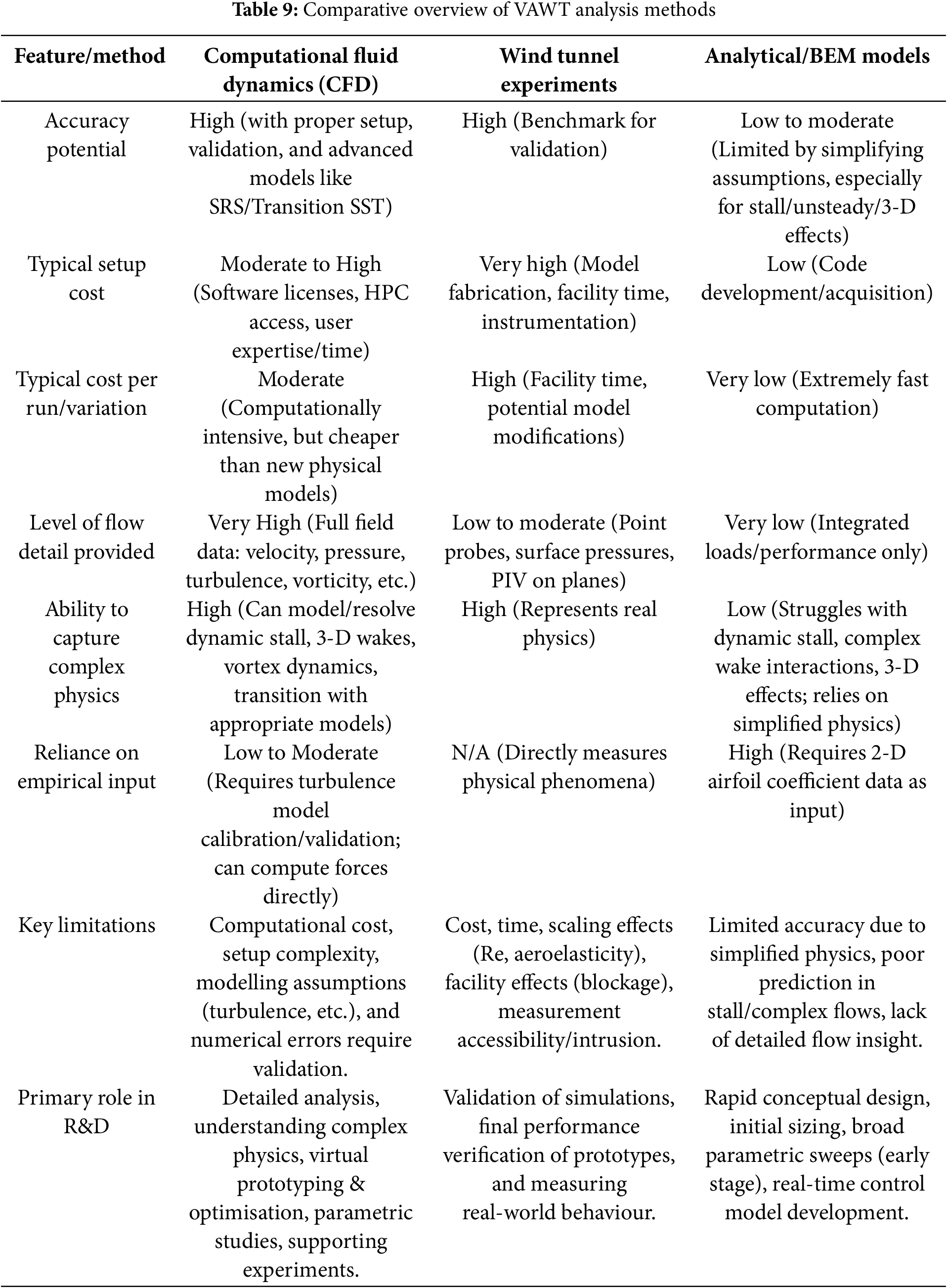
7  Gaps and Future Directions in VAWT CFD Research

While CFD modelling of VAWTs has advanced significantly, several challenges persist that define the future trajectory of research in this field. This section explicitly outlines the current limitations in VAWT CFD and identifies the emerging research directions aimed at overcoming these hurdles. The identified key gaps and limitations in current CFD modelling, and emerging and future research directions are outline in Tables 10 and 11, respectively.

8  Conclusion

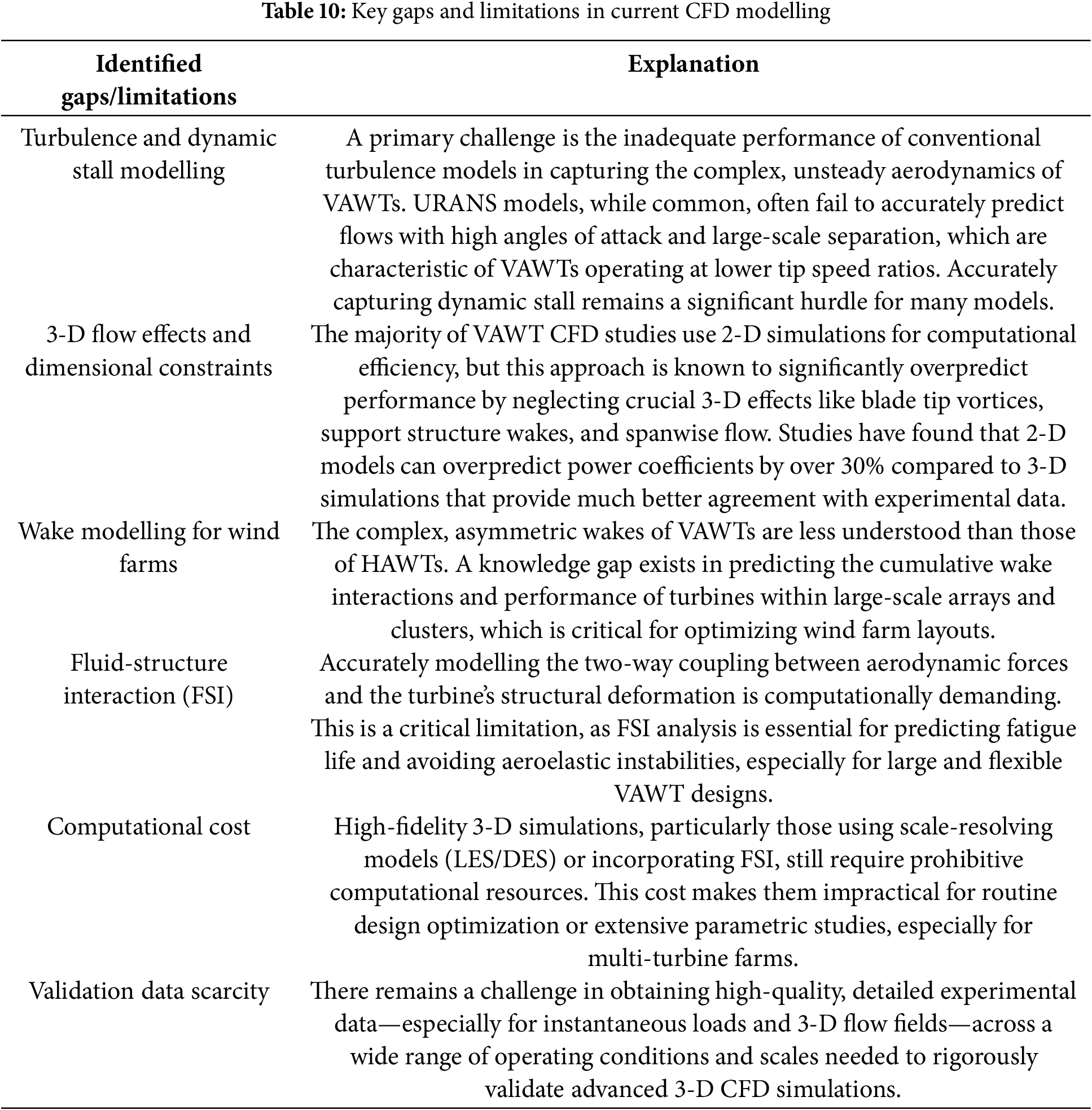
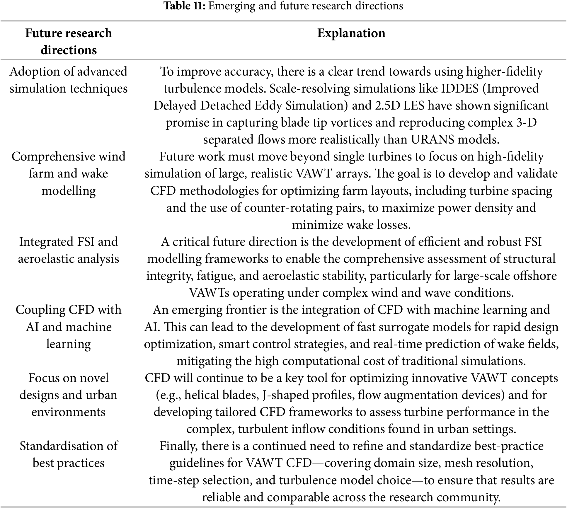
Computational fluid dynamics, firmly rooted in the fundamental laws of fluid motion has emerged as an indispensable technology for advancing the understanding and performance of vertical axis wind tur-bines. The inherent aerodynamic complexities of VAWTs, particularly the challenges posed by dynamic stall and intricate blade-wake interactions, often render traditional analytical methods insufficient and make purely experimental approaches costly and limited in scope. This review consolidates findings from over a hundred studies, providing a detailed account of how CFD has been utilized to address aerodynamic challenges such as dynamic stall, blade–wake interactions, unsteady loading, and low Reynolds number effects. Through improvements in meshing techniques, turbulence modeling, and transient simulation frameworks, CFD has enabled deeper insights into rotor aerodynamics, performance prediction, and design innovations.

Despite its advantages, CFD still faces several critical limitations when applied to VAWT analysis. One of the most prominent challenges is the high computational cost, particularly for three-dimensional, transient simulations required to accurately model complex flow phenomena such as dynamic stall, blade–wake interactions, and vortex shedding. These simulations demand significant processing time and memory, often limiting their feasibility to academic or small-scale investigations. Additionally, CFD outcomes are highly sensitive to mesh quality and domain size. Inadequate mesh resolution, especially near blade surfaces and in the wake region can result in inaccurate predictions of aerodynamic forces and power output. Furthermore, turbulence model selection remains a major source of uncertainty, as standard RANS models often struggle to capture unsteady flow separation, vortex dynamics, and tip losses accurately. While some progress has been made with hybrid and transition models, CFD simulations of VAWTs still require cautious interpretation and validation against experimental data to ensure reliability and confidence in the results.

To overcome current limitations and further enhance CFD’s role in VAWT research, future efforts should focus on incorporating high-fidelity turbulence models such as Large Eddy Simulation (LES) and Detached Eddy Simulation (DES). These models can resolve large-scale unsteady structures more accurately than RANS, improving the prediction of dynamic stall, wake recovery, and rotor–wake interactions. However, their adoption remains limited due to computational intensity, making hybrid RANS–LES approaches a promising compromise. Another significant research direction involves the integration of CFD with AI-driven optimization tools, including surrogate modeling, machine learning, and evolutionary algorithms. These frameworks can drastically reduce simulation time by guiding design iterations intelligently, enabling rapid evaluation of airfoil shapes, pitch angles, and array configurations. Finally, multidisciplinary co-simulation environments that couple CFD with structural dynamics, control systems, and even energy storage models could lead to comprehensive optimization of VAWT systems, particularly in urban or offshore applications where aerodynamic performance and structural robustness are equally critical.

In summary, while CFD has proven invaluable for VAWT development, further advancements in modeling strategies, computational efficiency, and intelligent automation are essential to fully unlock its potential in real-world applications.

Acknowledgement: The authors would like to acknowledge Universiti Kebangsaan Malaysia and Universiti Malaysia Sabah for providing the facilities used in this research.

Funding Statement: This research was funded by Ministry of Higher Education Malaysia under the Fundamental Research Grant Scheme (FRGS/1/2024/TK10/UKM/02/7).

Author Contributions: The authors confirm contribution to the paper as follows: Conceptualization, Wan Khairul Muzammil and Ahmad Fazlizan; methodology, Wan Khairul Muzammil; validation, data curation, Wan Khairul Muzammil; writing—review and editing, Ahmad Fazlizan, Najm Addin Al-Khawlani; visualization, Wan Khairul Muzammil and Ahmad Fazlizan; supervision, Wan Khairul Muzammil and Ahmad Fazlizan; project administration, Ahmad Fazlizan; funding acquisition, Ahmad Fazlizan. All authors reviewed the results and approved the final version of the manuscript.

Availability of Data and Materials: All data generated or analyzed during this study are included in this published article.

Ethics Approval: Not applicable.

Conflicts of Interest: The authors declare no conflicts of interest to report regarding the present study.

Nomenclature

References

1. Seifi Davari H, Seify Davari M, Botez RM, Chowdhury H. Advancements in vertical axis wind turbine technologies: a comprehensive review. Arab J Sci Eng. 2025;50(4):2169–216. doi:10.1007/s13369-024-09723-x. [Google Scholar] [CrossRef]

2. Chong WT, Muzammil WK, Ong HC, Sopian K, Gwani M, Fazlizan A, et al. Performance analysis of the deflector integrated cross axis wind turbine. Renew Energy. 2019;138(1):675–90. doi:10.1016/j.renene.2019.02.005. [Google Scholar] [CrossRef]

3. Chong WT, Yip SY, Fazlizan A, Poh SC, Hew WP, Tan EP, et al. Design of an exhaust air energy recovery wind turbine generator for energy conservation in commercial buildings. Renew Energy. 2014;67:252–6. doi:10.1016/j.renene.2013.11.028. [Google Scholar] [CrossRef]

4. Muralidhar Singh M, Hebbale AM, Durga Prasad C, Harish H, Kumar M, Shanthala K. Design and simulation of vertical axis windmill for streetlights. Mater Today Proc. 2023;92:73–7. doi:10.1016/j.matpr.2023.03.729. [Google Scholar] [CrossRef]

5. Vitali D, Garbuglia F, D’Alessandro V, Ricci R. The renewable energy in a led standalone streetlight. Int J Energy Prod Manag. 2017;2(1):118–8. doi:10.2495/EQ-V2-N1-118-128. [Google Scholar] [CrossRef]

6. Chong WT, Muzammil WK, Fazlizan A, Hassan MR, Taheri H, Gwani M, et al. Urban Eco-Greenergy™ hybrid wind-solar photovoltaic energy system and its applications. Int J Precis Eng Manuf. 2015;16(7):1263–8. doi:10.1007/s12541-015-0165-3. [Google Scholar] [CrossRef]

7. Kumar R, Raahemifar K, Fung AS. A critical review of vertical axis wind turbines for urban applications. Renew Sustain Energ Rev. 2018;89:281–91. doi:10.1016/J.RSER.2018.03.033. [Google Scholar] [CrossRef]

8. Li S, Chen Q, Li Y, Pröbsting S, Yang C, Zheng X, et al. Experimental investigation on noise characteristics of small scale vertical axis wind turbines in urban environments. Renew Energy. 2022;200(1):970–82. doi:10.1016/j.renene.2022.09.099. [Google Scholar] [CrossRef]

9. Hui I, Cain BE, Dabiri JO. Public receptiveness of vertical axis wind turbines. Energy Policy. 2018;112(4):258–71. doi:10.1016/j.enpol.2017.10.028. [Google Scholar] [CrossRef]

10. Ngouani Siewe MM, Chen YK, Day R, David-West O. CFD and experimental investigations of a novel vertical axis omni-flow wind turbine shroud system operating at low Reynolds numbers, typical urban flow conditions. Energy Convers Manag. 2025;326(24):119514. doi:10.1016/J.ENCONMAN.2025.119514. [Google Scholar] [CrossRef]

11. Sharpe T, Proven G. Crossflex: concept and early development of a true building integrated wind turbine. Energy Build. 2010;42(12):2365–75. doi:10.1016/j.enbuild.2010.07.032. [Google Scholar] [CrossRef]

12. Lawal R, Ige O, Adebayo S. Optimizing vertical axis wind turbines for urban environments: overcoming design challenges and maximizing efficiency in low-wind conditions. GSC Adv Res Rev. 2024;21(1):246–56. doi:10.30574/gscarr.2024.21.1.0384. [Google Scholar] [CrossRef]

13. Ibrahim AK, Saeed RI. A comprehensive review of vertical axis wind turbines for urban usage. Int J Novel Res Develop. 2022;7:336–43. [Google Scholar]

14. Yu H, Shao M, Jiang H. Numerical study on the time-harmonic gust response of a vertical axis wind turbine. Phys Fluids. 2025;37(1):015109. doi:10.1063/5.0244400. [Google Scholar] [CrossRef]

15. Saleh YAS, Durak M, Turhan C. Enhancing urban sustainability with novel vertical-axis wind turbines: a study on residential buildings in çeşme. Sustainability. 2025;17(9):3859. doi:10.3390/su17093859. [Google Scholar] [CrossRef]

16. Frunzulica F, Cismilianu A, Boros A, Dumitrache A, Suatean B. A new vertical axis wind turbine design for urban areas. AIP Conf Proc. 2016;1738:410008. doi:10.1063/1.4952209. [Google Scholar] [CrossRef]

17. Azadani LN. Vertical axis wind turbines in cluster configurations. Ocean Eng. 2023;272(4):113855. doi:10.1016/j.oceaneng.2023.113855. [Google Scholar] [CrossRef]

18. Barnes A, Marshall-Cross D, Hughes BR. Towards a standard approach for future Vertical Axis Wind Turbine aerodynamics research and development. Renew Sustain Energ Rev. 2021;148(4):111221. doi:10.1016/j.rser.2021.111221. [Google Scholar] [CrossRef]

19. Hand B. Three-dimensional computational fluid dynamic analysis of a large-scale vertical axis wind turbine. Wind Eng. 2022;46(2):572–97. doi:10.1177/0309524X211037911. [Google Scholar] [CrossRef]

20. Geng F, Suiker ASJ, Rezaeiha A, Montazeri H, Blocken B. A computational framework for the lifetime prediction of vertical-axis wind turbines: CFD simulations and high-cycle fatigue modeling. Int J Solids Struct. 2023;284(11):112504. doi:10.1016/j.ijsolstr.2023.112504. [Google Scholar] [CrossRef]

21. Tominaga Y. CFD prediction for wind power generation by a small vertical axis wind turbine: a case study for a university campus. Energies. 2023;16(13):4912. doi:10.3390/en16134912. [Google Scholar] [CrossRef]

22. Tu J, Yeoh GH, Liu C, Tao Y. Computational fluid dynamics: a practical approach. 4th ed. Oxford, UK: Elsevier; 2023. [Google Scholar]

23. Tinoco E. The role of computational fluid dynamics in aircraft design. In: Aerospace Engineering Conference and Show; 1990 Feb 13–15; Los Angela, CA, USA. [Google Scholar]

24. Anderson JD. Governing equations of fluid dynamics. In: Computational fluid dynamics. Berlin/Heidelberg, Germany: Springer; 1992. p. 15–51 doi:10.1007/978-3-662-11350-9_2. [Google Scholar] [CrossRef]

25. Ashgriz N, Mostaghimi J. An introduction to computational fluid dynamics. Fluid Flow Handbook. 2002;1:1–49. [Google Scholar]

26. Cadence CFD Solution. CFD simulation types: discretization, approximation, and algorithms [Internet]. 2020 [cited 2025 May 14]. Available from: https://resources.pcb.cadence.com/blog/2020-cfd-simulation-types-discretization-approximation-and-algorithms. [Google Scholar]

27. Sharma A. Introduction to computational fluid dynamics. In: Development, application and analysis. Cham, Switzerland: Springer; 2021. [Google Scholar]

28. Hunt JCR. Lewis fry richardson and his contributions to mathematics, meteorology, and models of conflict. Annu Rev Fluid Mech. 1998;30(1):xiii–xxxvi. doi:10.1146/annurev.fluid.30.1.0. [Google Scholar] [CrossRef]

29. Johnson NL. The legacy and future of CFD at Los Alamos. Los Alamos, NM, USA: Los Alamos National Lab; 1996. [Google Scholar]

30. Harlow FH. Fluid dynamics in group T-3 Los Alamos national laboratory: (LA-UR-03-3852). J Comput Phys. 2004;195:414–33. [Google Scholar]

31. Milne-Thomson LM. Theoretical aerodynamics. New York, NY, USA: Dover Publications; 1973. [Google Scholar]

32. McMurtry PA, Gansauge TC, Kerstein AR, Krueger SK. Linear eddy simulations of mixing in a homogeneous turbulent flow. Physics of Fluids A. 1992;5(4):1023–34. doi:10.1063/1.858667. [Google Scholar] [CrossRef]

33. Fimbres-Weihs GA, Wiley DE. Review of 3D CFD modeling of flow and mass transfer in narrow spacer-filled channels in membrane modules. Chem Eng Process Process Intensif. 2010;49(7):759–81. doi:10.1016/J.CEP.2010.01.007. [Google Scholar] [CrossRef]

34. Fang J, Brown C, Feng J, Li M, Bolotnov I. DNS of two-phase flow and growing HPC performance: review of capabilities and future outlook. In: 2017 Japan-US Seminar on Two-Phase Flow Dynamics; 2017 Jun 22–24; Hokkaido, Japan. [Google Scholar]

35. Sanderse B, Van der Pijl SP, Koren B. Review of computational fluid dynamics for wind turbine wake aerodynamics. Wind Energy. 2011;14(7):799–819. doi:10.1002/we.458. [Google Scholar] [CrossRef]

36. Miliket TA, Ageze MB, Tigabu MT. Aerodynamic performance enhancement and computational methods for H-Darrieus vertical axis wind turbines: review. Int J Green Energy. 2022;19(13):1428–65. doi:10.1080/15435075.2021.2005605. [Google Scholar] [CrossRef]

37. Menasri N, Zergane S, Aimeur N, Amour A. 3D CFD model for the analysis of the flow field through a horizontal axis wind turbine (HAWT). Acta Polytechnica. 2023;63(4). doi:10.14311/AP.2023.63.0250. [Google Scholar] [CrossRef]

38. Ajayi OA. Application of automotive alternators in small wind turbines [master's thesis]. Delft, The Netherlands: Delft University of Technology; 2012. [Google Scholar]

39. Buchner AJ, Soria J, Honnery D, Smits AJ. Dynamic stall in vertical axis wind turbines: scaling and topological considerations. J Fluid Mech. 2018;841:746. doi:10.1017/jfm.2018.112. [Google Scholar] [CrossRef]

40. Pan J, Ferreira C, van Zuijlen A. A numerical study on the blade-vortex interaction of a two-dimensional Darrieus-Savonius combined vertical axis wind turbine. Phys Fluids. 2023;35(12):125152. doi:10.1063/5.0174394. [Google Scholar] [CrossRef]

41. Abdolahifar A, Zanj A. Addressing VAWT aerodynamic challenges as the key to unlocking their potential in the wind energy sector. Energies. 2024;17(20):5052. doi:10.3390/en17205052. [Google Scholar] [CrossRef]

42. Fujisawa N, Shibuya S. Observations of dynamic stall on turbine blades. J Wind Eng Ind Aerodynamics. 2001;89(2):201–14. doi:10.1016/S0167-6105(00)00062-3. [Google Scholar] [CrossRef]

43. Lee K-Y, Cruden A, Ng J-H, Wong K-H. Variable designs of vertical axis wind turbines—a review. Front Energy Res. 2024;12:1437800. doi:10.3389/fenrg.2024.1437800. [Google Scholar] [CrossRef]

44. Rodriguez CV, Ríos A, Luyo JE. CFD design of urban wind turbines: a review and critical analysis. Int J Renew Ene Res. 2021;11(v11i2):618–38. doi:10.20508/ijrer.v11i2.11899.g8183. [Google Scholar] [CrossRef]

45. Gupta A, Ali U, Abderrahmane HA, Janajreh I. Blade pitching in vertical axis wind turbines: a double multiple stream tube theoretical approach to performance enhancement. Heliyon. 2025;11(3):e42101. doi:10.1016/J.HELIYON.2025.E42101. [Google Scholar] [PubMed] [CrossRef]

46. Tjiu W, Marnoto T, Mat S, Ruslan MH, Sopian K. Darrieus vertical axis wind turbine for power generation I: assessment of Darrieus VAWT configurations. Renew Energy. 2015;75:50–67. doi:10.1016/j.renene.2014.09.038. [Google Scholar] [CrossRef]

47. Murad N, Kamarudin MN, Rozali SM, Shaharudin NM. Review on wind turbine technology and control. J Adv Manufact Technol. 2017;11:87–100. [Google Scholar]

48. Eriksson S, Bernhoff H, Leijon M. Evaluation of different turbine concepts for wind power. Renew Sustain Energ Rev. 2008;12(5):1419–34. doi:10.1016/j.rser.2006.05.017. [Google Scholar] [CrossRef]

49. Chong W-T, Muzammil WK, Wong K-H, Wang C-T, Gwani M, Chu Y-J, et al. Cross axis wind turbine: pushing the limit of wind turbine technology with complementary design. Appl Energy. 2017;207(045306):78–95. doi:10.1016/j.apenergy.2017.06.099. [Google Scholar] [CrossRef]

50. Mitchell S, Ogbonna I, Volkov K. Improvement of self-starting capabilities of vertical axis wind turbines with new design of turbine blades. Sustainability. 2021;13(7):3854. doi:10.3390/su13073854. [Google Scholar] [CrossRef]

51. Huang H, Luo J, Li G. Study on the optimal design of vertical axis wind turbine with novel variable solidity type for self-starting capability and aerodynamic performance. Energy. 2023;271(1):127031. doi:10.1016/j.energy.2023.127031. [Google Scholar] [CrossRef]

52. Chegini S, Asadbeigi M, Ghafoorian F, Mehrpooya M. An investigation into the self-starting of Darrieus-savonius hybrid wind turbine and performance enhancement through innovative deflectors: a CFD approach. Ocean Eng. 2023;287(5):115910. doi:10.1016/j.oceaneng.2023.115910. [Google Scholar] [CrossRef]

53. Redchyts D, Portal-Porras K, Tarasov S, Moiseienko S, Tuchyna U, Starun N, et al. Aerodynamic performance of vertical-axis wind turbines. J Mar Sci Eng. 2023;11(7):1367. doi:10.3390/jmse11071367. [Google Scholar] [CrossRef]

54. Nobile R, Vahdati M, Barlow J, Mewburn-Crook A. Dynamic stall for a vertical axis wind turbine in a two-dimensional study. In: Proceedings of the World Renewable Energy Congress-Sweden; 2011 May 8–13; Linköping, Sweden. doi:10.3384/ecp110574225. [Google Scholar] [CrossRef]

55. Szczerba Z, Szczerba P, Szczerba K, Szumski M, Pytel K. Wind tunnel experimental study on the efficiency of vertical-axis wind turbines via analysis of blade pitch angle influence. Energies. 2023;16(13):4903. doi:10.3390/en16134903. [Google Scholar] [CrossRef]

56. Laneville A, Vittecoq P. Dynamic stall: the case of the vertical axis wind turbine. J Sol Energy Eng. 1986;108(2):140–5. doi:10.1115/1.3268081. [Google Scholar] [CrossRef]

57. Dunne R. Dynamic stall on vertical axis wind turbines [dissertation]. Pasadena, CA, USA: California Institute of Technology; 2016. [Google Scholar]

58. Simão Ferreira C, Van Kuik G, Van Bussel G, Scarano F. Visualization by PIV of dynamic stall on a vertical axis wind turbine. Exp Fluids. 2009;46(1):97–108. doi:10.1007/s00348-008-0543-z. [Google Scholar] [CrossRef]

59. Paraschivoiu I. Wind turbine design: with emphasis on Darrieus concept. Montréal, Canada: Presses Internationales Polytechnique; 2002. [Google Scholar]

60. Rezaeiha A, Montazeri H, Blocken B. Towards optimal aerodynamic design of vertical axis wind turbines: impact of solidity and number of blades. Energy. 2018;165(2):1129–48. doi:10.1016/j.energy.2018.09.192. [Google Scholar] [CrossRef]

61. Rolin V, Porté-Agel F. Wind-tunnel study of the wake behind a vertical axis wind turbine in a boundary layer flow using stereoscopic particle image velocimetry. J Phys Conf Ser. 2015;625(1):012012. doi:10.1088/1742-6596/625/1/012012. [Google Scholar] [CrossRef]

62. Barnes A, Marshall-Cross D, Hughes BR. Validation and comparison of turbulence models for predicting wakes of vertical axis wind turbines. J Ocean Eng Mar Energy. 2021;7(4):339–62. doi:10.1007/s40722-021-00204-z. [Google Scholar] [CrossRef]

63. Caprace DG, Winckelmans G, Chatelain P. An immersed lifting and dragging line model for the vortex particle-mesh method. Theor Comput Fluid Dyn. 2020;34(1–2):21–48. doi:10.1007/s00162-019-00510-1. [Google Scholar] [CrossRef]

64. Escudero Romero A, Blasetti AP, Acosta-López JG, Gómez-García M-Á, de Lasa H. Vorticity and its relationship to vortex separation, dynamic stall, and performance, in an H-Darrieus vertical-axis wind turbine using CFD simulations. Processes. 2024;12(8):1556. doi:10.3390/pr12081556. [Google Scholar] [CrossRef]

65. Zamre P, Lutz T. Computational-fluid-dynamics analysis of a Darrieus vertical-axis wind turbine installation on the rooftop of buildings under turbulent-inflow conditions. Wind Energy Sci. 2022;7(4):1661–77. doi:10.5194/wes-7-1661-2022. [Google Scholar] [CrossRef]

66. Wang Q, Liu B, Hu C, Wang F, Yang S. Aerodynamic shape optimization of H-VAWT blade airfoils considering a wide range of angles of attack. Int J Low Carbon Technol. 2022;17:147–59. doi:10.1093/ijlct/ctab092. [Google Scholar] [CrossRef]

67. Didane DH, Behery MR, Al-Ghriybah M, Manshoor B. Recent progress in design and performance analysis of vertical-axis wind turbines—a comprehensive review. Processes. 2024;12(6):1094. doi:10.3390/pr12061094. [Google Scholar] [CrossRef]

68. Rezaeiha A, Montazeri H, Blocken B. Towards accurate CFD simulations of vertical axis wind turbines at different tip speed ratios and solidities: guidelines for azimuthal increment, domain size and convergence. Energy Convers Manag. 2018;156(2):301–16. doi:10.1016/j.enconman.2017.11.026. [Google Scholar] [CrossRef]

69. Elsakka MM, Ingham DB, Ma L, Pourkashanian M. Comparison of the computational fluid dynamics predictions of vertical axis wind turbine performance against detailed pressure measurements. Int J Renew Energy Res. 2021;11(1):276–93. doi:10.20508/ijrer.v11i1.11755.g8131. [Google Scholar] [CrossRef]

70. Li C, Zhu S, Xu YL, Xiao Y. 2.5D large eddy simulation of vertical axis wind turbine in consideration of high angle of attack flow. Renew Energy. 2013;51(4):317–30. doi:10.1016/j.renene.2012.09.011. [Google Scholar] [CrossRef]

71. ed Fertahi SD, Belhadad T, Kanna A, Samaouali A, Kadiri I, Benini E. A critical review of CFD modeling approaches for Darrieus turbines: assessing discrepancies in power coefficient estimation and wake vortex development. Fluids. 2023;8(9):242. doi:10.3390/fluids8090242. [Google Scholar] [CrossRef]

72. Aihara A, Mendoza V, Goude A, Bernhoff H. Comparison of three-dimensional numerical methods for modeling of strut effect on the performance of a vertical axis wind turbine. Energies. 2022;15(7):2361. doi:10.3390/en15072361. [Google Scholar] [CrossRef]

73. Bianchini A, Balduzzi F, Bachant P, Ferrara G, Ferrari L. Effectiveness of two-dimensional CFD simulations for Darrieus VAWTs: a combined numerical and experimental assessment. Energy Convers Manag. 2017;136(12):318–28. doi:10.1016/j.enconman.2017.01.026. [Google Scholar] [CrossRef]

74. Giri Ajay A, Morgan L, Wu Y, Bretos D, Cascales A, Pires O, et al. Aerodynamic model comparison for an X-shaped vertical-axis wind turbine. Wind Energy Sci. 2024;9(2):453–70. doi:10.5194/wes-9-453-2024. [Google Scholar] [CrossRef]

75. Alaimo A, Esposito A, Messineo A, Orlando C, Tumino D. 3D CFD analysis of a vertical axis wind turbine. Energies. 2015;8(4):3013–33. doi:10.3390/en8043013. [Google Scholar] [CrossRef]

76. Belabes B, Paraschivoiu M. CFD modeling of vertical-axis wind turbine wake interaction. Transact Canadian Soc Mech Eng. 2023;47(4):449–58. doi:10.1139/tcsme-2022-0149. [Google Scholar] [CrossRef]

77. Simão Ferreira CJ, Bijl H, Van Bussel G, Van Kuik G. Simulating dynamic stall in a 2D VAWT: modeling strategy, verification and validation with Particle Image Velocimetry data. J Phys Conf Ser. 2007;75(1):012023. doi:10.1088/1742-6596/75/1/012023. [Google Scholar] [CrossRef]

78. Rezaeiha A, Kalkman I, Blocken B. CFD simulation of a vertical axis wind turbine operating at a moderate tip speed ratio: guidelines for minimum domain size and azimuthal increment. Renew Energy. 2017;107(1):373–85. doi:10.1016/j.renene.2017.02.006. [Google Scholar] [CrossRef]

79. Mo Q, Guan H, He S, Liu Y, Guo R. Guidelines for the computational domain size on an urban-scale VAWT. J Phys Conf Ser. 2021;1820(1):012177. doi:10.1088/1742-6596/1820/1/012177. [Google Scholar] [CrossRef]

80. kee Go W, Muhammad Hairi NB, Fazlizan A, Wong KH, Muzammil WK. Numerical analysis of the aerodynamic and geometric relationship of a vertical axis wind turbine. Transact Sci Technol. 2024;11:97–102. [Google Scholar]

81. Trebotich D, Graves DT. An adaptive finite volume method for the incompressible navier-stokes equations in complex geometries. Comm App Math Comp Sci. 2015;10(1):43–82. doi:10.2140/camcos.2015.10.43. [Google Scholar] [CrossRef]

82. Ma L, Wang X, Zhu J, Kang S. Dynamic stall of a vertical-axis wind turbine and its control using plasma actuation. Energies. 2019;12(19):3738. doi:10.3390/en12193738. [Google Scholar] [CrossRef]

83. Bang CS, Rana ZA, Prince SA. CFD analysis on novel vertical axis wind turbine (VAWT). Machines. 2024;12(11):800. doi:10.3390/machines12110800. [Google Scholar] [CrossRef]

84. Lam HF, Peng HY. Study of wake characteristics of a vertical axis wind turbine by two- and three-dimensional computational fluid dynamics simulations. Renew Energy. 2016;90:386–98. doi:10.1016/j.renene.2016.01.011. [Google Scholar] [CrossRef]

85. Almohammadi KM, Ingham DB, Ma L, Pourkashan M. Computational fluid dynamics (CFD) mesh independency techniques for a straight blade vertical axis wind turbine. Energy. 2013;58(1):483–93. doi:10.1016/j.energy.2013.06.012. [Google Scholar] [CrossRef]

86. Nobile R, Vahdati M, Barlow JF, Mewburn-Crook A. Unsteady flow simulation of a vertical axis augmented wind turbine: a two-dimensional study. J Wind Eng Ind Aerodyn. 2014;125:168–79. doi:10.1016/J.JWEIA.2013.12.005. [Google Scholar] [CrossRef]

87. Castelli MR, Masi M, Battisti L, Benini E, Brighenti A, Dossena V, et al. Reliability of numerical wind tunnels for VAWT simulation. J Phys Conf Ser. 2016;753(8):082025. doi:10.1088/1742-6596/753/8/082025. [Google Scholar] [CrossRef]

88. Elmekawy AMN, Saeed HAH, Kassab SZ. Performance enhancement of Savonius wind turbine by blade shape and twisted angle modifications. Proc Institut Mech Eng Part A J Pow Energy. 2021;235(6):1487–500. doi:10.1177/0957650920987942. [Google Scholar] [CrossRef]

89. Carrigan TJ, Dennis BH, Han ZX, Wang BP. Aerodynamic shape optimization of a vertical-axis wind turbine using differential evolution. ISRN Renew Energy. 2012;2012(1):528418. doi:10.5402/2012/528418. [Google Scholar] [CrossRef]

90. Bianchini A, Balduzzi F, Haack L, Bigalli S, Müller B, Ferrara G. Development and validation of a hybrid simulation model for Darrieus vertical-axis wind turbines. In: ASME Turbo Expo 2019: Turbomachinery Technical Conference and Exposition; 2017 Jul 17–21; Phoenix, AZ, USA. doi:10.1115/GT2019-91218. [Google Scholar] [CrossRef]

91. Mejia ODL, Mejia OE, Escorcia KM, Suarez F, Laín S. Comparison of sliding and overset mesh techniques in the simulation of a vertical axis turbine for hydrokinetic applications. Processes. 2021;9(11):1933. doi:10.3390/pr9111933. [Google Scholar] [CrossRef]

92. Song C, Zheng Y, Zhao Z, Zhang Y, Li C, Jiang H. Investigation of meshing strategies and turbulence models of computational fluid dynamics simulations of vertical axis wind turbines. J Renew Sustain Energy. 2015;7(3):033111. doi:10.1063/1.4921578. [Google Scholar] [CrossRef]

93. Balduzzi F, Bianchini A, Maleci R, Ferrara G, Ferrari L. Critical issues in the CFD simulation of Darrieus wind turbines. Renew Energy. 2016;85(1):419–35. doi:10.1016/j.renene.2015.06.048. [Google Scholar] [CrossRef]

94. Burg C, Erwin T. Application of Richardson extrapolation to the numerical solution of partial differential equations. Numer Methods Partial Differ Equ. 2009;25(4):810–32. doi:10.1002/num.20375. [Google Scholar] [CrossRef]

95. Meana-Fernández A, Fernández Oro JM, Argüelles Díaz KM, Velarde-Suárez S. Turbulence-model comparison for aerodynamic-performance prediction of a typical vertical-axis wind-turbine airfoil. Energies. 2019;12(3):488. doi:10.3390/en12030488. [Google Scholar] [CrossRef]

96. Baker N, Kelly G, O’Sullivan PD. A grid convergence index study of mesh style effect on the accuracy of the numerical results for an indoor airflow profile. Int J Vent. 2020;19(4):300–14. doi:10.1080/14733315.2019.1667558. [Google Scholar] [CrossRef]

97. Liu Q, Miao W, Ye Q, Li C. Performance assessment of an innovative Gurney flap for straight-bladed vertical axis wind turbine. Renew Energy. 2022;185(117):1124–38. doi:10.1016/j.renene.2021.12.098. [Google Scholar] [CrossRef]

98. Králik J. CFD simulation of air flow over an object with gable roof, revised with Y+ approach. Trans VŠB. 2016;16(2):85–94. doi:10.1515/tvsb-2016-0018. [Google Scholar] [CrossRef]

99. Zadeh SN, Komeili M, Paraschivoiu M. Mesh convergence study for 2-D straight-blade vertical axis wind turbine simulations and estimation for 3-D simulations. Trans Can Soc Mech Eng. 2014;38(4):487–504. doi:10.1139/tcsme-2014-0032. [Google Scholar] [CrossRef]

100. Zadeh MN, Pourfallah M, Sabet SS, Gholinia M, Mouloodi S, Ahangar AT. Performance assessment and optimization of a helical Savonius wind turbine by modifying the Bach’s section. SN Appl Sci. 2021;3(8):739. doi:10.1007/s42452-021-04731-0. [Google Scholar] [CrossRef]

101. Priyadumkol J, Muangput B, Namchanthra S, Zin T, Phengpom T, Chookaew W, et al. CFD modelling of vertical-axis wind turbines using transient dynamic mesh towards lateral vortices capturing and Strouhal number. Energy Convers Manag X. 2025;26(2):101022. doi:10.1016/j.ecmx.2025.101022. [Google Scholar] [CrossRef]

102. Bangga G, Lutz T, Dessoky A, Krämer E. Unsteady Navier-Stokes studies on loads, wake, and dynamic stall characteristics of a two-bladed vertical axis wind turbine. J Renew Sustain Energy. 2017;9(5):053303. doi:10.1063/1.5003772. [Google Scholar] [CrossRef]

103. Almohammadi KM, Ingham DB, Ma L, Pourkashanian M. Modeling dynamic stall of a straight blade vertical axis wind turbine. J Fluids Struct. 2015;57:144–58. doi:10.1016/j.jfluidstructs.2015.06.003. [Google Scholar] [CrossRef]

104. Hansen MOL, Sørensen JN, Voutsinas S, Sørensen N, Madsen HA. State of the art in wind turbine aerodynamics and aeroelasticity. Prog Aerosp Sci. 2006;42(4):285–330. doi:10.1016/j.paerosci.2006.10.002. [Google Scholar] [CrossRef]

105. Ferziger JH, Perić M, Street RL. Computational methods for fluid dynamics. Berlin/Heidelberg, Germany: Springer; 1996. [Google Scholar]

106. Trivellato F, Raciti Castelli M. On the Courant-Friedrichs–Lewy criterion of rotating grids in 2D vertical-axis wind turbine analysis. Renew Energy. 2014;62(3):53–62. doi:10.1016/j.renene.2013.06.022. [Google Scholar] [CrossRef]

107. Scheurich F, Brown RE. Modelling the aerodynamics of vertical-axis wind turbines in unsteady wind conditions. Wind Energy. 2013;16(1):91–107. doi:10.1002/we.532. [Google Scholar] [CrossRef]

108. Wong KH, Chong WT, Poh SC, Shiah YC, Sukiman NL, Wang CT. 3D CFD simulation and parametric study of a flat plate deflector for vertical axis wind turbine. Renew Energy. 2018;129(2):32–55. doi:10.1016/j.renene.2018.05.085. [Google Scholar] [CrossRef]

109. Jin G, Zong Z, Jiang Y, Zou L. Aerodynamic analysis of side-by-side placed twin vertical-axis wind turbines. Ocean Eng. 2020;209(7):107296. doi:10.1016/j.oceaneng.2020.107296. [Google Scholar] [CrossRef]

110. Gupta A, Abderrahmane HA, Janajreh I. Flow analysis and sensitivity study of vertical-axis wind turbine under variable pitching. Appl Energy. 2024;358(8):122648. doi:10.1016/j.apenergy.2024.122648. [Google Scholar] [CrossRef]

111. Ullah T, Javed A, Abdullah A, Ali M, Uddin E. Computational evaluation of an optimum leading-edge slat deflection angle for dynamic stall control in a novel urban-scale vertical axis wind turbine for low wind speed operation. Sustain Energy Technol Assess. 2020;40(9):100748. doi:10.1016/j.seta.2020.100748. [Google Scholar] [CrossRef]

112. Benmoussa A, Páscoa JC. Enhancement of a cycloidal self-pitch vertical axis wind turbine performance through DBD plasma actuators at low tip speed ratio. Int J Thermofluids. 2023;17(8):100258. doi:10.1016/j.ijft.2022.100258. [Google Scholar] [CrossRef]

113. McLaren K, Tullis S, Ziada S. Computational fluid dynamics simulation of the aerodynamics of a high solidity, small-scale vertical axis wind turbine. Wind Energy. 2012;15(3):349–61. doi:10.1002/we.472. [Google Scholar] [CrossRef]

114. Zereg A, Lebaal N, Aksas M, Derradji B, Chabani I, Mebarek-Oudina F. CFD analysis of a vertical axis wind turbine. In: Mathematical modelling of fluid dynamics and nanofluids. Boca Raton, FL, USA: CRC Press; 2023. p. 184–96. doi:10.1201/9781003299608-12. [Google Scholar] [CrossRef]

115. Lin Z, Qian L, Campobasso MS, Bai W, Zhou Y, Ma Z. Modelling aerodynamics of a floating offshore wind turbine using the overset mesh solver in OpenFOAM. In: ASME 2022 41st International Conference on Ocean, Offshore and Arctic Engineering; 2022 Jun 5–10; Hamburg, Germany. doi:10.1115/omae2022-79230. [Google Scholar] [CrossRef]

116. Lei H, Zhou D, Bao Y, Chen C, Ma N, Han Z. Numerical simulations of the unsteady aerodynamics of a floating vertical axis wind turbine in surge motion. Energy. 2017;127(3):1–17. doi:10.1016/j.energy.2017.03.087. [Google Scholar] [CrossRef]

117. Lei H, Zhou D, Lu J, Chen C, Han Z, Bao Y. The impact of pitch motion of a platform on the aerodynamic performance of a floating vertical axis wind turbine. Energy. 2017;119(2–3):369–83. doi:10.1016/j.energy.2016.12.086. [Google Scholar] [CrossRef]

118. Laws P, Saini JS, Kumar A, Mitra S. Improvement in savonius wind turbines efficiency by modification of blade designs—a numerical study. J Energy Resour Technol. 2020;142(6):061303. doi:10.1115/1.4045476. [Google Scholar] [CrossRef]

119. Leonczuk Minetto RA, Paraschivoiu M. Simulation based analysis of morphing blades applied to a vertical axis wind turbine. Energy. 2020;202(11):117705. doi:10.1016/j.energy.2020.117705. [Google Scholar] [CrossRef]

120. Gomes T, Lemaire S, Vaz G. Code and solution verification of sliding and overset grid methods on wind turbine flows. In: ASME 2022 41st International Conference on Ocean, Offshore and Arctic Engineering; 2022 Jun 5–10; Hamburg, Germany. doi:10.1115/omae2022-81337. [Google Scholar] [CrossRef]

121. Marchewka E, Sobczak K, Reorowicz P, Obidowski D, Krzysztof J. Application of overset mesh approach in the investigation of the Savonius wind turbines with rigid and deformable blades. Arch Thermodyn. 2023;42(4):201–16. doi:10.24425/ather.2021.139659. [Google Scholar] [CrossRef]

122. Elbeji T, Ben Amira W, Souaissa K, Ghiss M, Bentaher H, Ben Fredj N. Three-dimensional aeroelastic investigation of a novel convex bladed H-Darrieus wind turbine based on a two-way coupled computational fluid dynamics and finite element analysis approach. Fluids. 2025;10(1):17. doi:10.3390/fluids10010017. [Google Scholar] [CrossRef]

123. Abd-Elhay MSE. Fluid-structure interaction of NREL 5-MW wind turbine [master’s thesis]. Cairo, Egypt: The American University in Cairo; 2021. [Google Scholar]

124. Zhang X, Wang Z, Li W. Structural optimization of H-type VAWT blade under fluid-structure interaction conditions. J Vibroeng. 2021;23(5):1207–18. doi:10.21595/jve.2021.21766. [Google Scholar] [CrossRef]

125. Baghdadi M, Elkoush S, Akle B, Elkhoury M. Dynamic shape optimization of a vertical-axis wind turbine via blade morphing technique. Renew Energy. 2020;154(9):239–51. doi:10.1016/j.renene.2020.03.015. [Google Scholar] [CrossRef]

126. Nunez EE, García González D, López OD, Casas Rodríguez JP, Laín S. Fluid-structure interaction of a Darrieus-type hydrokinetic turbine modified with winglets. J Mar Sci Eng. 2025;13(3):548. doi:10.3390/jmse13030548. [Google Scholar] [CrossRef]

127. Franchina N, Kouaissah O, Persico G, Savini M. Three-dimensional CFD simulation and experimental assessment of the performance of a H-shape vertical-axis wind turbine at design and off-design conditions. Int J Turbomach Propuls Power. 2019;4(3):30. doi:10.3390/ijtpp4030030. [Google Scholar] [CrossRef]

128. Buchner AJ, Lohry MW, Martinelli L, Soria J, Smits AJ. Dynamic stall in vertical axis wind turbines: comparing experiments and computations. J Wind Eng Ind Aerodyn. 2015;146(1):163–71. doi:10.1016/j.jweia.2015.09.001. [Google Scholar] [CrossRef]

129. Ashwindran S, Azizuddin AA, Oumer AN. Computational fluid dynamic (CFD) of vertical-axis wind turbine: mesh and time-step sensitivity study. J Mech Eng Sci. 2019;13(3):5604–24. doi:10.15282/jmes.13.3.2019.24.0450. [Google Scholar] [CrossRef]

130. Pandey A, Scheel JD, Schumacher J. Turbulent superstructures in Rayleigh-Bénard convection. Nat Commun. 2018;9(1):2118. doi:10.1038/s41467-018-04478-0. [Google Scholar] [PubMed] [CrossRef]

131. Elsakka MM, Ingham DB, Ma L, Pourkashanian M. Effects of turbulence modelling on the predictions of the pressure distribution around the wing of a small scale vertical axis wind turbine. In: Proceedings of the 6th European Conference on Computational Mechanics: Solids, Structures and Coupled Problems, ECCM 2018 and 7th European Conference on Computational Fluid Dynamics, ECFD 2018; 2018 Jun 11–15; Glasgow, UK. [Google Scholar]

132. Rosa RMS. Turbulence theories. In: Encyclopedia of mathematical physics. Amsterdam, The Netherlands: Elsevier; 2006. p. 295–303. doi:10.1016/b0-12-512666-2/00111-5. [Google Scholar] [CrossRef]

133. Zhang C, Bounds CP, Foster L, Uddin M. Turbulence modeling effects on the CFD predictions of flow over a detailed full-scale Sedan vehicle. Fluids. 2019;4(3):148. doi:10.3390/fluids4030148. [Google Scholar] [CrossRef]

134. Rands C, Webb BW, Maynes D. Characterization of transition to turbulence in microchannels. Int J Heat Mass Transf. 2006;49(17–18):2924–30. doi:10.1016/j.ijheatmasstransfer.2006.02.032. [Google Scholar] [CrossRef]

135. Santamaría L, Galdo Vega M, Pandal A, González Pérez J, Velarde-Suárez S, Fernández Oro JM. Aerodynamic performance of VAWT airfoils: comparison between wind tunnel testing using a new three-component strain gauge balance and CFD modelling. Energies. 2022;15(24):9351. doi:10.3390/en15249351. [Google Scholar] [CrossRef]

136. Schovanec C, Agarwal RK. CFD modeling of a vertical axis wind turbine near highway traffic using actuator cylinder theory. In: AIAA AVIATION 2021 FORUM; 2021 Aug 2–6; Reston, VA, USA. doi:10.2514/6.2021-2593. [Google Scholar] [CrossRef]

137. Rezaeiha A, Montazeri H, Blocken B. On the accuracy of turbulence models for CFD simulations of vertical axis wind turbines. Energy. 2019;180(8):838–57. doi:10.1016/j.energy.2019.05.053. [Google Scholar] [CrossRef]

138. Syawitri TP, Yao YF, Chandra B, Yao J. Comparison study of URANS and hybrid RANS-LES models on predicting vertical axis wind turbine performance at low, medium and high tip speed ratio ranges. Renew Energy. 2021;168(1):247–69. doi:10.1016/j.renene.2020.12.045. [Google Scholar] [CrossRef]

139. Syawitri TP, Yao Y, Yao J, Chandra B. Assessment of stress-blended eddy simulation model for accurate performance prediction of vertical axis wind turbine. Int J Numer Meth Heat Fluid Flow. 2021;31(2):655–73. doi:10.1108/hff-09-2019-0689. [Google Scholar] [CrossRef]

140. Mauro S, Brusca S, Lanzafame R, Messina M. Micro H-Darrieus wind turbines: CFD modeling and experimental validation. In: AIP Conference Proceedings. Erode, India: AIP Publishing; 2019. doi:10.1063/1.5138842. [Google Scholar] [CrossRef]

141. Li QA, Maeda T, Kamada Y, Murata J, Kawabata T, Shimizu K, et al. Wind tunnel and numerical study of a straight-bladed vertical axis wind turbine in three-dimensional analysis (Part I: for predicting aerodynamic loads and performance). Energy. 2016;106(4):443–52. doi:10.1016/j.energy.2016.03.089. [Google Scholar] [CrossRef]

142. Rashed MR, Abdellatif OE, Abd Rabbo MF, Khalil EE, Shahin I. Turbulence modeling comparative analysis for vertical axis wind turbines. Eng Res J Fac Eng Shoubra. 2020;44(1):71–9. doi:10.21608/erjsh.2020.290027. [Google Scholar] [CrossRef]

143. Wilcox D. A half century historical review of the k-omega model. In: 29th Aerospace Sciences Meeting; 1991 Jan 7–10; Reston, VA, USA. doi:10.2514/6.1991-615. [Google Scholar] [CrossRef]

144. Syawitri TP, Yao Y, Yao J, Chandra B. A review on the use of passive flow control devices as performance enhancement of lift-type vertical axis wind turbines. Wires Energy Environ. 2022;11(4):e435. doi:10.1002/wene.435. [Google Scholar] [CrossRef]

145. Menter FR. Two-equation eddy-viscosity turbulence models for engineering applications. AIAA J. 1994;32(8):1598–605. [Google Scholar]

146. Jafaryar M, Kamrani R, Gorji-Bandpy M, Hatami M, Ganji DD. Numerical optimization of the asymmetric blades mounted on a vertical axis cross-flow wind turbine. Int Commun Heat Mass Transf. 2016;70(2):93–104. doi:10.1016/j.icheatmasstransfer.2015.12.003. [Google Scholar] [CrossRef]

147. Abdalkarem AAM, Fazlizan A, Muzammil WK, Lim CH, Ibrahim A, Wong KH, et al. The effect of various wedge flap configurations on the performance of wind turbine airfoil. Iran J Sci Technol Trans Mech Eng. 2024;48(4):1879–99. doi:10.1007/s40997-023-00743-w. [Google Scholar] [CrossRef]

148. Yamin M, Putra A, Firmansyah R. 2D CFD simulation on the aerodynamic performance enhancement of H-Darrieus VAWT utilized with flaps. Eng Sci Lett. 2024;3(3):91–9. doi:10.56741/esl.v3i03.564. [Google Scholar] [CrossRef]

149. Rezaeiha A, Montazeri H, Blocken B. Numerical simulations of vertical axis wind turbines using different turbulence models. In: International Symposium on Computational Wind Engineering (CWE2018); 2018 Jun 18–22; Seoul, Republic of Korea. [Google Scholar]

150. Tan W, Zhang H, Wang L, Nie S, Jiao J, Zuo Y. Effects of the uncertainty of wall distance on the simulation of turbulence/transition phenomena. Aerospace. 2024;11(11):898. doi:10.3390/aerospace11110898. [Google Scholar] [CrossRef]

151. Galetta M. Impact of dynamic stall on VAWT performance: implementation into a double multiple stream-tube tool and quantification of model uncertainty [master's thesis]. Milan, Italy: Politecnico di Milano; 2019. [Google Scholar]

152. Liu B, Vanierschot M, Buysschaert F. Comparison study of the k-kL–ω and γ–Reθ transition model in the open-water performance prediction of a rim-driven thruster. Int J Turbomach Propuls Power. 2024;9(1):2. doi:10.3390/ijtpp9010002. [Google Scholar] [CrossRef]

153. Khani S, Porté-Agel F. A gradient tensor-based subgrid-scale parameterization for large-eddy simulations of stratified shear layers using the weather research and forecasting model. Mon Weather Rev. 2022;150(9):2279–98. doi:10.1175/mwr-d-21-0217.1. [Google Scholar] [CrossRef]

154. Amalia E, Moelyadi MA, Ihsan M. Effects of turbulence model and numerical time steps on von karman flow behavior and drag accuracy of circular cylinder. J Phys Conf Ser. 2018;1005:012012. doi:10.1088/1742-6596/1005/1/012012. [Google Scholar] [CrossRef]

155. Lanzafame R, Mauro S, Messina M, Brusca S. Development and validation of CFD 2D models for the simulation of micro H-Darrieus turbines subjected to high boundary layer instabilities. Energies. 2020;13(21):5564. doi:10.3390/en13215564. [Google Scholar] [CrossRef]

156. Patankar SV, Spalding DB. A calculation procedure for heat, mass and momentum transfer in three-dimensional parabolic flows. Int J Heat Mass Transf. 1972;15(10):1787–806. doi:10.1016/0017-9310(72)90054-3. [Google Scholar] [CrossRef]

157. Hsu CJ. Numerical heat transfer and fluid flow. Nucl Sci Eng. 1981;78(2):196–7. doi:10.13182/nse81-a20112. [Google Scholar] [CrossRef]

158. Van Doormaal JP, Raithby GD. Enhancements of the simple method for predicting incompressible fluid flows. Numer Heat Transf. 1984;7(2):147–63. doi:10.1080/01495728408961817. [Google Scholar] [CrossRef]

159. Issa RI. Solution of the implicitly discretised fluid flow equations by operator-splitting. J Comput Phys. 1986;62(1):40–65. doi:10.1016/0021-9991(86)90099-9. [Google Scholar] [CrossRef]

160. Rezaeiha A, Kalkman I, Blocken B. Effect of pitch angle on power performance and aerodynamics of a vertical axis wind turbine. Appl Energy. 2017;197(8):132–50. doi:10.1016/j.apenergy.2017.03.128. [Google Scholar] [CrossRef]

161. Simão Ferreira CJ, van Zuijlen A, Bijl H, van Bussel G, van Kuik G. Simulating dynamic stall in a two-dimensional vertical-axis wind turbine: verification and validation with particle image velocimetry data. Wind Energy. 2010;13(1):1–17. doi:10.1002/we.330. [Google Scholar] [CrossRef]

162. Chowdhury AM, Akimoto H, Hara Y. Comparative CFD analysis of vertical axis wind turbine in upright and tilted configuration. Renew Energy. 2016;85(1):327–37. doi:10.1016/j.renene.2015.06.037. [Google Scholar] [CrossRef]

163. Concli F, Gorla C, Della Torre A, Montenegro G. Churning power losses of ordinary gears: a new approach based on the internal fluid dynamics simulations. Lubr Sci. 2015;27(5):313–26. doi:10.1002/ls.1280. [Google Scholar] [CrossRef]

164. Branlard E. Wind turbine aerodynamics and vorticity-based methods: fundamentals and recent applications. Cham, Switzerland: Springer International Publishing; 2017. [Google Scholar]

165. Rahman M, Salyers TE, El-Shahat A, Ilie M, Ahmed M, Soloiu V. Numerical and experimental investigation of aerodynamic performance of vertical-axis wind turbine models with various blade designs. J Power Energy Eng. 2018;6(5):26–63. doi:10.4236/jpee.2018.65003. [Google Scholar] [CrossRef]

166. Hosseini Rad S, Ghafoorian F, Taraghi M, Moghimi M, Ghoveisi Asl F, Mehrpooya M. A systematic study on the aerodynamic performance enhancement in H-type Darrieus vertical axis wind turbines using Vortex cavity layouts and deflectors. Phys Fluids. 2024;36(12):125170. doi:10.1063/5.0243164. [Google Scholar] [CrossRef]

167. Kong Z, Zhou D, Sun X. Improvement of self-starting and power extraction performance of an H-type vertical-axis hydrokinetic turbine by partial deflection of its blades. Ocean Eng. 2024;296:116855. doi:10.1016/j.oceaneng.2024.116855. [Google Scholar] [CrossRef]

168. Wisner KS, Yu M. Vertical-axis turbine performance enhancement with physics-informed blade pitch control. Basic principles and proof of concept with high-fidelity numerical simulation. J Renew Sustain Energy. 2024;16(2):023305. doi:10.1063/5.0178535. [Google Scholar] [CrossRef]

169. Sun X, Xu Y, Huang D. Numerical simulation and research on improving aerodynamic performance of vertical axis wind turbine by co-flow jet. J Renew Sustain Energy. 2019;11(1):013303. doi:10.1063/1.5052378. [Google Scholar] [CrossRef]

170. Zhu H, Hao W, Li C, Ding Q. Numerical study of effect of solidity on vertical axis wind turbine with Gurney flap. J Wind Eng Ind Aerodyn. 2019;186(1):17–31. doi:10.1016/j.jweia.2018.12.016. [Google Scholar] [CrossRef]

171. Abdolahifar A, Karimian SMH. A comprehensive three-dimensional study on Darrieus vertical axis wind turbine with slotted blade to reduce flow separation. Energy. 2022;248(6):123632. doi:10.1016/j.energy.2022.123632. [Google Scholar] [CrossRef]

172. Wang Z, Zhuang M. Leading-edge serrations for performance improvement on a vertical-axis wind turbine at low tip-speed-ratios. Appl Energy. 2017;208:1184–97. doi:10.1016/j.apenergy.2017.09.034. [Google Scholar] [CrossRef]

173. Chong WT, Fazlizan A, Poh SC, Pan KC, Hew WP, Hsiao FB. The design, simulation and testing of an urban vertical axis wind turbine with the omni-direction-guide-vane. Appl Energy. 2013;112:601–9. doi:10.1016/j.apenergy.2012.12.064. [Google Scholar] [CrossRef]

174. de Santoli L, Albo A, Astiaso Garcia D, Bruschi D, Cumo F. A preliminary energy and environmental assessment of a micro wind turbine prototype in natural protected areas. Sustain Energy Technol Assess. 2014;8(2):42–56. doi:10.1016/j.seta.2014.07.002. [Google Scholar] [CrossRef]

175. Singh SV, Kumar P. Study of flow characteristics of a savonius turbine inside nozzle diffuser duct. J Eng Res. 2022. doi:10.36909/jer.15977. [Google Scholar] [CrossRef]

176. Dessoky A, Bangga G, Lutz T, Krämer E. Aerodynamic and aeroacoustic performance assessment of H-rotor Darrieus VAWT equipped with wind-lens technology. Energy. 2019;175(1):76–97. doi:10.1016/j.energy.2019.03.066. [Google Scholar] [CrossRef]

177. Aboujaoude H, Beaumont F, Murer S, Polidori G, Bogard F. Aerodynamic performance enhancement of a Savonius wind turbine using an axisymmetric deflector. J Wind Eng Ind Aerodyn. 2022;220(5):104882. doi:10.1016/j.jweia.2021.104882. [Google Scholar] [CrossRef]

178. Li Y, Tong G, Ma Y, Feng F, Tagawa K. Numerical study on aerodynamic performance improvement of the straight-bladed vertical axis wind turbine by using wind concentrators. Renew Energy. 2023;219(4):119545. doi:10.1016/j.renene.2023.119545. [Google Scholar] [CrossRef]

179. Deda Altan B, Gungor A. Improvement of Savonius wind turbine performance with using wind collector. Sci Iran. 2023. doi:10.24200/sci.2023.60454.6809. [Google Scholar] [CrossRef]

180. Xu Z, Dong X, Li K, Zhou Q, Zhao Y. Study of the self-starting performance of a vertical-axis wind turbine. J Appl Fluid Mech. 2024;17(6):1261–76. doi:10.47176/jafm.17.6.2295. [Google Scholar] [CrossRef]

181. Fatahian E, Mishra R, Jackson FF, Fatahian H. Optimization and analysis of self-starting capabilities of vertical axis wind turbine pairs: a CFD-Taguchi approach. Ocean Eng. 2024;302(1–3):117614. doi:10.1016/j.oceaneng.2024.117614. [Google Scholar] [CrossRef]

182. Uma Reddy K, Deb B, Roy B. A numerical and experimental study on the performance of a conventional H- Darrieus wind rotor with auxiliary blades. Ocean Eng. 2023;280:114697. doi:10.1016/j.oceaneng.2023.114697. [Google Scholar] [CrossRef]

183. Worasinchai S, Ingram GL, Dominy RG. The physics of H-Darrieus turbine starting behavior. J Eng Gas Turbines Power. 2016;138(6):062605. [Google Scholar]

184. Hill N, Dominy R, Ingram G, Dominy J. Darrieus turbines: the physics of self-starting. Proc Inst Mech Eng Part A J Power Energy. 2009;223(1):21–9. doi:10.1243/09576509jpe615. [Google Scholar] [CrossRef]

185. Celik Y, Ma L, Ingham D, Pourkashanian M. Aerodynamic investigation of the start-up process of H-type vertical axis wind turbines using CFD. J Wind Eng Ind Aerodyn. 2020;204:104252. doi:10.1016/j.jweia.2020.104252. [Google Scholar] [CrossRef]

186. Lunt PAV. An aerodynamic model for a vertical-axis wind turbine. MEng Project Report. Durham, UK: School of Engineering, Durham University; 2005. [Google Scholar]

187. Yousefi Roshan M, Khaleghinia J, Eshagh Nimvari M, Salarian H. Performance improvement of Darrieus wind turbine using different cavity layouts. Energy Convers Manag. 2021;246(4):114693. doi:10.1016/j.enconman.2021.114693. [Google Scholar] [CrossRef]

188. Farzadi R, Bazargan M. 3D numerical simulation of the Darrieus vertical axis wind turbine with J-type and straight blades under various operating conditions including self-starting mode. Energy. 2023;278(1):128040. doi:10.1016/j.energy.2023.128040. [Google Scholar] [CrossRef]

189. Al-Gburi KAH, Alnaimi FBI, Al-quraishi BAJ, Tan ES, Kareem AK. Enhancing savonius vertical axis wind turbine performance: a comprehensive approach with numerical analysis and experimental investigations. Energies. 2023;16(10):4204. doi:10.3390/en16104204. [Google Scholar] [CrossRef]

190. Fatahian H, Mishra R, Jackson FF, Fatahian E. Design optimization of an innovative deflector with bleed jets to enhance the performance of dual Savonius turbines using CFD-Taguchi method. Energy Convers Manag. 2023;296(3):117655. doi:10.1016/j.enconman.2023.117655. [Google Scholar] [CrossRef]

191. Peng HY, Han ZD, Liu HJ, Lin K, Lam HF. Assessment and optimization of the power performance of twin vertical axis wind turbines via numerical simulations. Renew Energy. 2020;147:43–54. doi:10.1016/j.renene.2019.08.124. [Google Scholar] [CrossRef]

192. Cheng B, Du J, Yao Y. Power prediction formula for blade design and optimization of dual Darrieus wind turbines based on taguchi method and genetic expression programming model. Renew Energy. 2022;192(10):583–605. doi:10.1016/j.renene.2022.04.111. [Google Scholar] [CrossRef]

193. Shrestha S, Manogharan G. Optimization of binder jetting using taguchi method. JOM. 2017;69(3):491–7. doi:10.1007/s11837-016-2231-4. [Google Scholar] [CrossRef]

194. Suprianto FD, Chern MJ, Wang CC. Parametric study of passive flow enhancement on a Magnus VAWT blade using response surface methodology and direct-forcing immersed boundary method. J Renewable Sustainable Energy. 2024;16(2):023302. doi:10.1063/5.0189589. [Google Scholar] [CrossRef]

195. Sarkar D, Shukla S, Alom N, Sharma P, Bora BJ. Investigation of a newly developed slotted bladed Darrieus vertical axis wind turbine: a numerical and response surface methodology analysis. J Energy Resour Technol. 2023;145(5):051302. doi:10.1115/1.4056331. [Google Scholar] [CrossRef]

196. Trentin PFS, de Barros Martinez PHB, dos Santos GB, Gasparin EE, Salviano LO. Screening analysis and unconstrained optimization of a small-scale vertical axis wind turbine. Energy. 2022;240:122782. doi:10.1016/j.energy.2021.122782. [Google Scholar] [CrossRef]

197. Zhang R, Kuang L, Tu Y, Dong Z, Ping H, Zhang K, et al. Multiple boundary layer suction slots technique for performance improvement of vertical-axis wind turbines: conceptual design and parametric analysis. Phys Fluids. 2024;36(7):075126. doi:10.1063/5.0214013. [Google Scholar] [CrossRef]

198. El Maani R, Radi B, El Hami A. Numerical study and optimization-based sensitivity analysis of a vertical-axis wind turbine. Energies. 2024;17(24):6300. doi:10.3390/en17246300. [Google Scholar] [CrossRef]

199. Ghoneam S, Hamada A, Sherif T. Modeling and optimization for the dynamic performance of vertical-axis wind turbine composite blades. J Sol Energy Eng. 2021;143(2):021005. doi:10.1115/1.4048159. [Google Scholar] [CrossRef]

200. Ahmad M, Shahzad A, Akram F, Qadri MNM. Determination of efficient configurations of vertical axis wind turbine using design of experiments. Proc Inst Mech Eng Part A J Power Energy. 2022;236(8):1558–81. doi:10.1177/09576509221095347. [Google Scholar] [CrossRef]

201. Asadbeigi M, Ghafoorian F, Mehrpooya M, Chegini S, Jarrahian A. A 3D study of the Darrieus wind turbine with auxiliary blades and economic analysis based on an optimal design from a parametric investigation. Sustainability. 2023;15(5):4684. doi:10.3390/su15054684. [Google Scholar] [CrossRef]

202. Lu X, Xu S. Performance optimization of vertical axis wind turbine based on Taguchi method, improved differential evolution algorithm and Kriging model. Energy Sources Part A Recovery Util Environ Eff. 2024;46(1):2792–810. doi:10.1080/15567036.2024.2308655. [Google Scholar] [CrossRef]

203. Chen Y, Zhang D, Li X, Peng Y, Zhang X, Han Z, et al. Surrogate models for twin-VAWT performance based on Kriging and artificial neural networks. Ocean Eng. 2023;273(2):113947. doi:10.1016/j.oceaneng.2023.113947. [Google Scholar] [CrossRef]

204. Ghoneam SM, Hamada AA, Sherif TS. Fatigue-life estimation of vertical-axis wind turbine composite blades using modal analysis. J Energy Resour Technol. 2024;146(3):031301. doi:10.1115/1.4064178. [Google Scholar] [CrossRef]

205. Wang Q, Zhang Z. Airfoil optimization design of vertical-axis wind turbine based on Kriging surrogate model and MIGA. Energies. 2025;18(11):2927. doi:10.3390/en18112927. [Google Scholar] [CrossRef]

206. Rezaeiha A, Montazeri H, Blocken B. CFD analysis of dynamic stall on vertical axis wind turbines using Scale-Adaptive Simulation (SAScomparison against URANS and hybrid RANS/LES. Energy Convers Manag. 2019;196(1):1282–98. doi:10.1016/j.enconman.2019.06.081. [Google Scholar] [CrossRef]

207. Wilberforce T, Alaswad A. Performance analysis of a vertical axis wind turbine using computational fluid dynamics. Energy. 2023;263(4):125892. doi:10.1016/j.energy.2022.125892. [Google Scholar] [CrossRef]

208. Li Z, Han R, Gao P, Wang C. Analysis and implementation of a drag-type vertical-axis wind turbine for small distributed wind energy systems. Adv Mech Eng. 2019;11(1):1687814019825709. doi:10.1177/1687814019825709. [Google Scholar] [CrossRef]

209. Franchina N, Persico G, Savini M. 2D-3D computations of a vertical axis wind turbine flow field: modeling issues and physical interpretations. Renew Energy. 2019;136(8):1170–89. doi:10.1016/j.renene.2018.09.086. [Google Scholar] [CrossRef]

210. Zhang X, Sun X. Performance enhancement of an H-Darrieus vertical axis wind turbine via moving surface boundary-layer control. Energy Sci Eng. 2023;11(3):1180–201. doi:10.1002/ese3.1384. [Google Scholar] [CrossRef]

211. Rezaeiha A, Montazeri H, Blocken B. CFD simulations of a vertical axis wind turbine in dynamic stall: URANS vs. scale-adaptive simulation (SAS). In: 7th Symposium on Hybrid RANS/LES Methods (HRLM2018); 2018 Sep 17–21; Berlin, Germany. [Google Scholar]

212. Dabiri JO. Potential order-of-magnitude enhancement of wind farm power density via counter-rotating vertical-axis wind turbine arrays. J Renew Sustain Energy. 2011;3(4):043104. doi:10.1063/1.3608170. [Google Scholar] [CrossRef]

213. Kouaissah O, Franchina N, Persico G. A computational fluid dynamics study on the performance of modified H-shaped VAWTs for tilted operation condition. J Eng Gas Turbines Power. 2025;147(5):051017. doi:10.1115/1.4066615. [Google Scholar] [CrossRef]

214. Dewan A, Tomar SS, Bishnoi AK, Singh TP. Computational fluid dynamics and turbulence modelling in various blades of Savonius turbines for wind and hydro energy: progress and perspectives. Ocean Eng. 2023;283(1):115168. doi:10.1016/j.oceaneng.2023.115168. [Google Scholar] [CrossRef]

215. Tian W, Song B, VanZwieten J, Pyakurel P. Computational fluid dynamics prediction of a modified savonius wind turbine with novel blade shapes. Energies. 2015;8(8):7915–29. doi:10.3390/en8087915. [Google Scholar] [CrossRef]

216. Tian W, Ni X, Mao Z, Wang YF. Study on the performance of a new VAWT with overlapped side-by-side Savonius rotors. Energy Convers Manag. 2022;264(1):115746. doi:10.1016/j.enconman.2022.115746. [Google Scholar] [CrossRef]

217. Akhlaghi M, Asadbeigi M, Ghafoorian F. Novel CFD and DMST dual method parametric study and optimization of a Darrieus vertical axis wind turbine. J Appl Fluid Mech. 2024;17(1). doi:10.47176/jafm.17.1.1985. [Google Scholar] [CrossRef]

218. Arpino F, Cortellessa G, Massarotti N, Mauro A, Scungio M. Numerical performance assessment of a novel Darrieus-style VAWT with auxiliary straight blades. J Phys Conf Ser. 2020;1589(1):012020. doi:10.1088/1742-6596/1589/1/012020. [Google Scholar] [CrossRef]

219. Acosta-López JG, Blasetti AP, Lopez-Zamora S, de Lasa H. CFD modeling of an H-type Darrieus VAWT under high winds: the vorticity index and the imminent Vortex separation condition. Processes. 2023;11(2):644. doi:10.3390/pr11020644. [Google Scholar] [CrossRef]

220. Arpino F, Cortellessa G, Scungio M, Fresilli G, Facci A, Frattolillo A. PIV measurements over a double bladed Darrieus-type vertical axis wind turbine: a validation benchmark. Flow Meas Instrum. 2021;82(5):102064. doi:10.1016/j.flowmeasinst.2021.102064. [Google Scholar] [CrossRef]

221. Ahmad M, Rehman I. Investigating aerodynamic performance of vertical axis wind turbines using computational techniques. J Power Gener Technol. 2023;1(1):20. doi:10.61369/jpgt.0568. [Google Scholar] [CrossRef]

222. Farajyar S, Ghafoorian F, Mehrpooya M, Asadbeigi M. CFD investigation and optimization on the aerodynamic performance of a savonius vertical axis wind turbine and its installation in a hybrid power supply system: a case study in Iran. Sustainability. 2023;15(6):5318. doi:10.3390/su15065318. [Google Scholar] [CrossRef]

223. Fertahi SE, Samaouali A, Kadiri I. CFD comparison of 2D and 3D aerodynamics in H-Darrieus prototype wake. E Prime Adv Electr Eng Electron Energy. 2023;4(4):100178. doi:10.1016/j.prime.2023.100178. [Google Scholar] [CrossRef]

224. Ferreira CS, van Bussel G, Van Kuik G. 2D CFD simulation of dynamic stall on a vertical axis wind turbine: verification and validation with PIV measurements. In: 45th AIAA Aerospace Sciences Meeting and Exhibit; 2007 Jan 8–11; Reno, Nevada. doi:10.2514/6.2007-1367. [Google Scholar] [CrossRef]

225. Chen Y, Lian Y. Numerical investigation of Vortex dynamics in an H-rotor vertical axis wind turbine. Eng Appl Comput Fluid Mech. 2015;9(1):21–32. doi:10.1080/19942060.2015.1004790. [Google Scholar] [CrossRef]

226. Eftekhari H, Al-Obaidi ASM, Eftekhari S. Aerodynamic performance of vertical and horizontal axis wind turbines: a comparison review. Indonesian J Sci Technol. 2021;7(1):65–88. doi:10.17509/ijost.v7i1.43161. [Google Scholar] [CrossRef]