Deep Learning Model for Identifying Internal Flaws Based on Image Quadtree SBFEM and Deep Neural Networks

1  Introduction

Due to the experience of natural disasters, oxidation, corrosion, material degradation and continuous loading, structures in the process of long-term service may gradually develop inconspicuous internal flaws, such as micro-cracks and voids. These flaws often degrade the local strength and stability of the structure, or even result in catastrophic failures. As a pivotal link in ensuring structural safety and quality, identification of flaws and damage in critical structure components has long been a research focus in the field of structural health monitoring. In recent years, nondestructive testing technologies for structures have been widely applied in various fields, including civil engineering, water conservancy, transportation, aerospace, and mechanical engineering. The main non-destructive testing methods include ultrasonic testing [1,2], ground-penetrating radar [3,4], infrared imaging [5,6], and acoustic emission testing [7,8]. Among these methods, internal flaws are identified by analyzing the responses of materials or structures to external signals based on their physical properties, which can be regarded as direct detection of damaged regions within the structure. Additionally, inverse analysis of internal flaws in structures can be conducted based on the external responses of the structure [9,10].

With the advancement of computer technology, many scholars have conducted relevant research and achieved promising results. Ma et al. [11] proposed a flaw inversion model for detection of multiple complex flaw clusters based on the extended finite element method (XFEM) and the artificial bee colony algorithm. The hierarchical clustering analysis was conducted to capture potential subdomains containing flaws and the positions of complex flaw clusters in structures can be located effectively. Subsequently, Zhao et al. [12] employed XFEM to solve the forward problems of flaw detection and used the K-means clustering algorithm to estimate the number of flaws. The proposed approach not only detected the positions of complex-shaped flaws in structures, but also significantly improved the convergence speed of flaw inversion. A couple of method of the level set method with the finite element method was proposed by Zhang et al. [13] for identifying two-dimensional and three-dimensional holes in structures. To a certain extent, the aforementioned studies have preliminarily addressed the issues of quantitative inversion of flaw information in the field of nondestructive testing. However, when the traditional finite element methods are employed in those numerical models, the meshes or integration regions usually need to be regenerated or adjusted for fitting well with geometric boundaries. What’s worse, the flaw detection iterative process usually contains hundreds and thousands of forward analyses to obtain defect parameters within the allowable error range. The computational workload is huge and it would be heavier due to the complex shapes and the unknown number of flaws.

To reduce computational costs, several studies combined artificial intelligence algorithms with the computational mechanics model to identify flaws [14,15]. Dong et al. [16] utilized Convolutional Neural Networks (CNNs) to propose a localizing and classifying model of anomalies in the industrial component inspection task. The performance was capable both at the pixel level (localizing flawed regions) and the image level (identifying whether an image contains flaws). Yang et al. [17] integrated a deep learning feature extraction method with the Extreme Learning Machine (ELM) classification approach to establish a deep extreme learning machine model for flaw detection in wood images. This model achieved a flaw recognition accuracy of 96.72% for wood, with a testing time of only 187 ms. Nguyen-Ngoc et al. [18] proposed a new Structural Health Monitoring (SHM) damage detection method for truss bridges by coupling a DNN model with the evolved Artificial Rabbit Optimization (EVARO) algorithm, which demonstrated excellent performance in damage localization and quantification. Huang et al. [19] employed artificial neural networks to determine the severity of damage. This method can accurately identify damage in beam structures using only a small amount of displacement data. The average error between the obtained damage severity and the true value does not exceed 4%. In conclusion, it’s feasible to establish the flaw detection model by combining computational mechanics and artificial intelligence algorithms. The nonlinear mapping relationships are revealed between structural responses and flaw parameters.

Therefore, we take the advantages of artificial intelligence algorithms and SBFEM to set up the deep learning model for identifying internal flaws. The scaled boundary finite element method (SBFEM) is an alternative method with a semi-analytical accuracy in calculation [20], which exhibits outstanding works on automatic flaw/damage simulations [21,22]. Combined with the quadtree algorithm and SBFEM, only 6 types of unique elements are needed to cover all mesh morphologies and all the shapes are square [23–25]. The handing node is common with the regular node and doesn’t affect the calculation accuracy. It overcomes the difficulties of low data generation efficiency and complex interface processing to a certain extent. On the other hand, we utilize DNN as the learning framework and employ a Bayesian regularization algorithm to suppress the risk of local convergence of the objective function. A deep learning model for square plates with flaws is established to accurately locate and quantify the size of flaws in the structure. In addition, we analyze the impact of the number of training set samples and flaw size on the inversion results, providing insights for the research on structural disaster prevention and mitigation technologies that combine computational mechanics methods with DNNs.

2  Basic Theory of the SBFEM

SBFEM is an alternative method that is analogous to the finite element method. In the solution process, the computational domain is discretized into multiple S-elements. Subsequently, the stiffness matrices of these individual S-elements are assembled to solve for the unknowns. When performing calculations using SBFEM, only the boundaries of the structural domain require discretization. Hanging nodes can be directly treated as regular nodes, which endows it with unique advantages in addressing complex material interfaces and problems involving singularities [26].

In the local coordinate system ξ Oη, ξ denotes the radial coordinate, where ξ = 0 is at the scaling center and ξ = 1 at the polygon boundary, and η is the circumferential coordinate along the polygon boundary. Within a two-dimensional finite domain, for a Cartesian coordinate system xOy, the coordinate values x and y of any arbitrary point inside an element can be expressed in the local coordinate system:

x=ξxb(η)=ξN(η)xb(1)

y=ξyb(η)=ξN(η)yb(2)

where N(η) is the shape functions with N(η)=[N1(η),N2(η),⋯], xb and yb denote the nodal coordinates vectors of the two-node line element on the boundary with xb=[x1,x2]T, yb=[y1,y2]T.

With the coordinate transformation to the scaled boundary coordinate, the displacements at point inside the subdomain are formed as

u(ξ,η)=N(η)u(ξ)(3)

where u(ξ) is the analytical displacements on the radial direction.

Based on the principle of virtual work, the two-dimensional linear elastic static equilibrium equation for SBFEM can be derived.

E0ξ2u(ξ),ξξ+(E0+E1T−E1)ξu(ξ),ξ−E2u(ξ)=0(4)

where E0, E1 and E2 are coefficient matrices, which are similar to the static stiffness matrices in finite element method (FEM) [26].

When solving using SBFEM, the coefficient matrices are determined solely by the boundary conditions and material parameters of the computational domain. Eq. (4) is transformed into a first-order differential equation.

ξX(ξ),ξ=−Z{u(ξ)q(ξ)}(5)

where q(ξ) is the equivalent internal force vector and the Hamiltonian coefficient matrix Z is

Z=[−E0−1E1TE0−1E2−E1E0−1E1TE1E0−1](6)

The displacements u(ξ) can be obtained by solving the eigenvalues of the Hamiltonian matrix.

u(ξ)=Ψnξ−Snc(7)

where Ψn is the modal displacement vector. Sn is the positive real part of the eigenvalue vector of the modal displacement. c is the integral constant vector.

3  SBFEM Based on Image Quadtree Algorithm

The quadtree mesh generation algorithm is a method that enables rapid transition between coarse and fine meshes in different computational regions by controlling thresholds. High-quality square meshes are generated by the quadtree algorithm and it can be directly converted into SBFEM subdomains. The resulting hanging nodes are treated as regular nodes without affecting solution accuracy. Considering the rotation and symmetry of square meshes, the quadtree mesh generation process only involves six types of node arrangements. When performing linear elastic analysis using SBFEM, only these six element patterns need to be calculated, with no special treatment required [27,28].

A DNN for plate-like structures with circular holes is established based on SBFEM combined with an image quadtree approach. Training the model requires generating a large number of training samples in a short period. Image quadtree SBFEM offers unique advantages when solving problems related to plate-like structures with circular holes [29,30]. It allows direct mesh generation on the image structure, thereby reducing the modeling time for irregular structural models. During mesh generation, only local refinement of the mesh at material interfaces is necessary, which reduces the number of mesh elements and significantly lowers computational costs [31].

Using the image quadtree SBFEM approach, quadtree mesh generation is performed on the image of a heterogeneous concrete aggregate model with double holes. The left end of the model is fixed, and a uniformly distributed load of P = 1 MPa is applied at the right end. The color inside the holes is represented by 255, while that of the matrix is represented by 0. The maximum element size is set to 32, the minimum to 1, and the threshold to 0.05. The completed quadtree mesh, as shown in Fig. 1a, consists of 102,921 elements in total. All calculations in this study were conducted on a desktop PC equipped with an Intel(R) Core (TM) i7-8700 CPU @ 3.20 GHz and 64 GB of RAM. The contour plot of the structural horizontal displacement obtained from static calculations is illustrated in Fig. 1b, with a computational time of only 5.372 s.

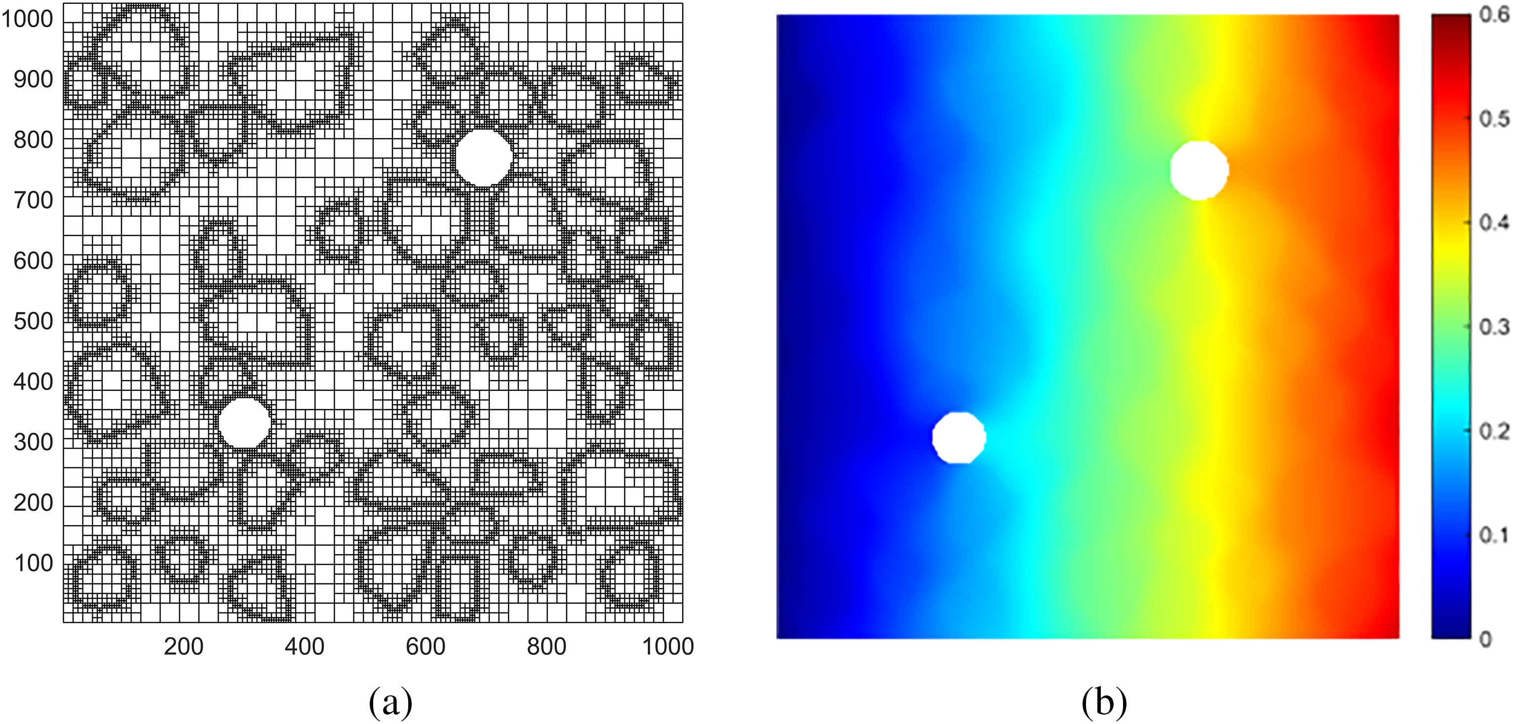
Figure 1: (a) Quadtree mesh containing double holes; (b) Contour plot of horizontal displacement for the square plate

4  DNN-Based Structural Flaw Inversion Model

In DNNs, mathematical transformations are achieved by stacking different layers and adjusting the weights of each layer through functions, thereby describing data patterns. In this chapter, the image quadtree SBFEM is used to calculate the displacement responses of structural observation points under different loads. Based on a DNN with a backpropagation algorithm, an inversion model for internal flaws or damaged areas of the structure is constructed.

4.1 Structural Design of DNN for Flaw Inversion

The displacement responses of observation points are used as data features, and flaw parameters as data labels, to jointly train the DNN model. This process is essentially an inverse analysis. The mathematical model for deriving flaw position parameters is expressed as follows:

minpE(p)s.t.g(p)=0,h(p)≤0(8)

where p represents the vector of structural flaw parameters (e.g., the location, size, shape, and number of flaws). g(p) is the mechanical equilibrium equation of the image quadtree SBFEM. h(p) is used to limit the feasible range of flaw parameters. E(p) refers to the objective function constructed from observed and predicted values:

E(p)=12∑i=1n(ui−ui(p))2(9)

where ui is the observed value at the i-th observation point (e.g., displacement, strain), and ui(p) is the simulated value obtained via forward numerical calculation based on the flaw parameter p.

The weighted Mean Squared Error (MSE) is adopted to assign different weight coefficients to the output target based on the magnitude of the target variable and the task requirements. For a two-dimensional flaw inversion problem, the flaw region may be defined by the parameter p = [x, y, r] (the center position and radius of the circular flaw), and the MSE is:

MSE=w1⋅MSEx+w2⋅MSEy+w3⋅MSEr(10)

To avoid ill-posed problems or non-unique solutions in the calculation process, a regularization term is added to the objective function E(p), which can then be rewritten as:

Ereg(p)=E(p)+λR(p)(11)

For example, for a single flaw board with three flaw parameters x, y, and r, the reverse analysis mathematical model can be expressed as:

minx,y,r=12∑i=1n(uiobs−uisim(x,y,r))2+λ(x2+y2+r2)(12)

Once the model objective function is established, the network parameters of the DNN are set based on the flaw parameters predicted by the inversion model. During the entire training process, the Bayesian regularization algorithm is introduced for gradient update in back propagation to construct the model’s loss function E, and the Adam algorithm is used for optimization:

E=βED+αEW(13)

where the regularization parameters α and β are dynamically adjusted via Bayesian regularization during network training to balance error minimization and weight constraints. ED is the error between the network output and the target value, and EW is the weight regularization term used to constrain the weight magnitude:

ED=12∑n=1N∑m=13(ym(n)−y^m(n))2(14)

EW=12(∑i,jωij2+∑k,iωki2+∑m,kωmk2)(15)

The establishment process of the DNN is shown in Fig. 2:

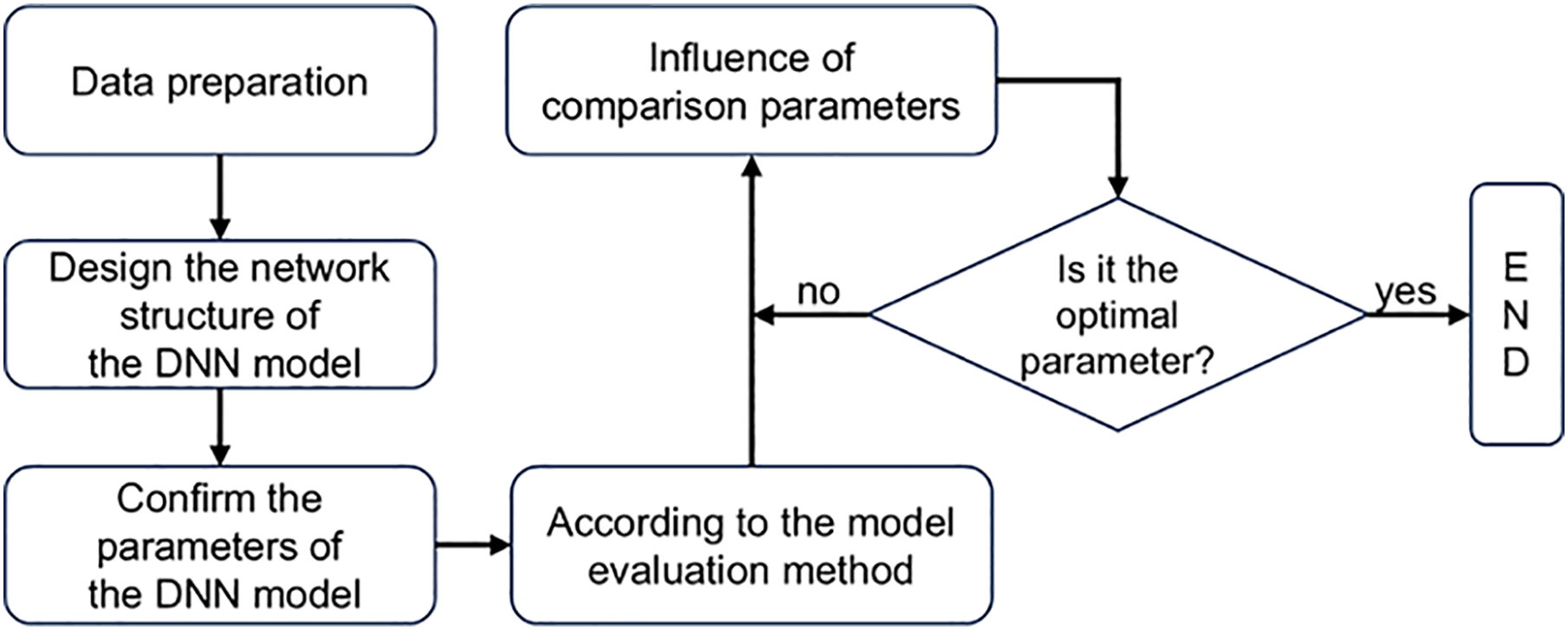
Figure 2: Flowchart of DNN model establishment

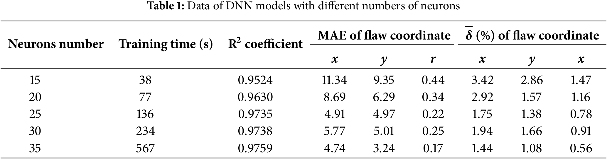
The sample dataset of the single-flaw inversion model is used as comparative optimization data. After the model’s objective function is established, the network parameters of DNN are set according to the flaw parameters predicted by the inversion model. Herein, the deep learning model contains two hidden layers. The Adam algorithm is used throughout the training process to optimize the loss function. The tanh function is employed as the activation function of the deep learning model and grid search is used as the optimization algorithm. In order to select the feasible number of neurons in hidden layers, a comparative analysis is conducted in terms of training time, Mean Absolute Error (MAE) and the average relative error δ¯. The number of iterations is 500 and the number of neurons is set to 15, 20, 25, 30, and 35, respectively. R2 coefficient is employed to evaluate the model’s ability to explain the variation in the dependent variable. The training time and R2 coefficient of the DNN model are counted. The MAE and average relative error δ¯ between the predicted parameters and the true values are calculated, respectively. The statistical results are shown in Table 1. When the number of neurons exceeds 25, the MAE and average relative error between the predicted values and the true values are not significantly different. When 30 or more neurons are used, the model training takes more time. Therefore, it is considered to set the number of neurons in both hidden layers to 25.

4.2 Flaw Inversion Stages

As shown in Fig. 3, the model can be divided into two stages: preprocessing and inversion.

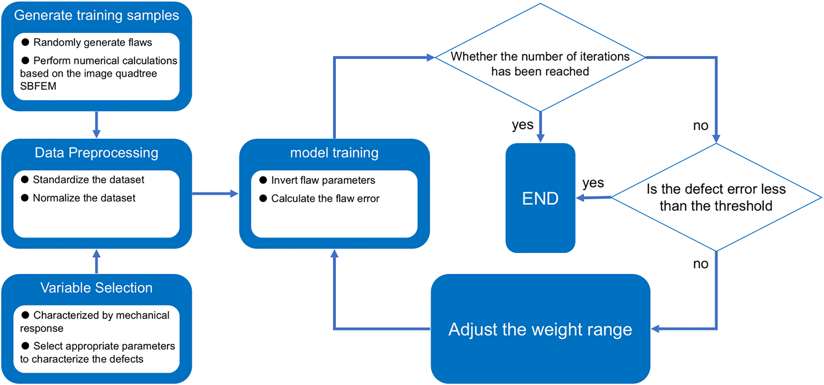
Figure 3: Model inversion flowchart

(1)   The preprocessing stage of this paper is as follows: A large number of square plates with unknown circular flaws are randomly generated. The left end of each flawed plate is fixed, and a uniformly distributed load is applied to the right end. Six observation points are evenly arranged on the upper and lower boundaries of the flawed plate. Numerical simulations are performed on the flawed plates using the image-based quadtree SBFEM to obtain the displacements at the observation points. These displacements are used as input features, and the positions and sizes of the flaws as output labels. A large dataset is generated by repeating this process. The generated dataset is then standardized such that the input feature values are scaled to the range [0, 1], and the output labels to the range [−1, 1]. The standardized dataset is used to train the designed DNN model, where the weights and bias parameters of each part of the DNN model are fitted to establish a nonlinear mapping between the responses at the observation points and the flaw parameters. At this stage, the trained DNN model can output the corresponding flaw parameters given only the responses at the observation points.

(2)   Inversion Stage: The test set data divided during the preprocessing stage is input into the trained DNN model. The DNN model automatically outputs the flaw parameters, thereby completing the inversion of flaw information.

5  Numerical Examples

5.1 Inversion of Single Circular Flaw

As shown in Fig. 4, a square plate with a single circular flaw is considered, with a side length of a = 1000 mm. The left end of the plate is fixed, and a uniformly distributed load of P = 100 MPa is applied at the right end. Six observation points are evenly distributed along the upper and lower boundaries of the plate. The elastic modulus of the plate is E = 210 GPa, and Poisson’s ratio is ν = 0.3. The internal flaw under study is a circular hole, described by three parameters: the center coordinates and radius r of the flaw. The flaw radius r ranges from 15 to 50 mm.

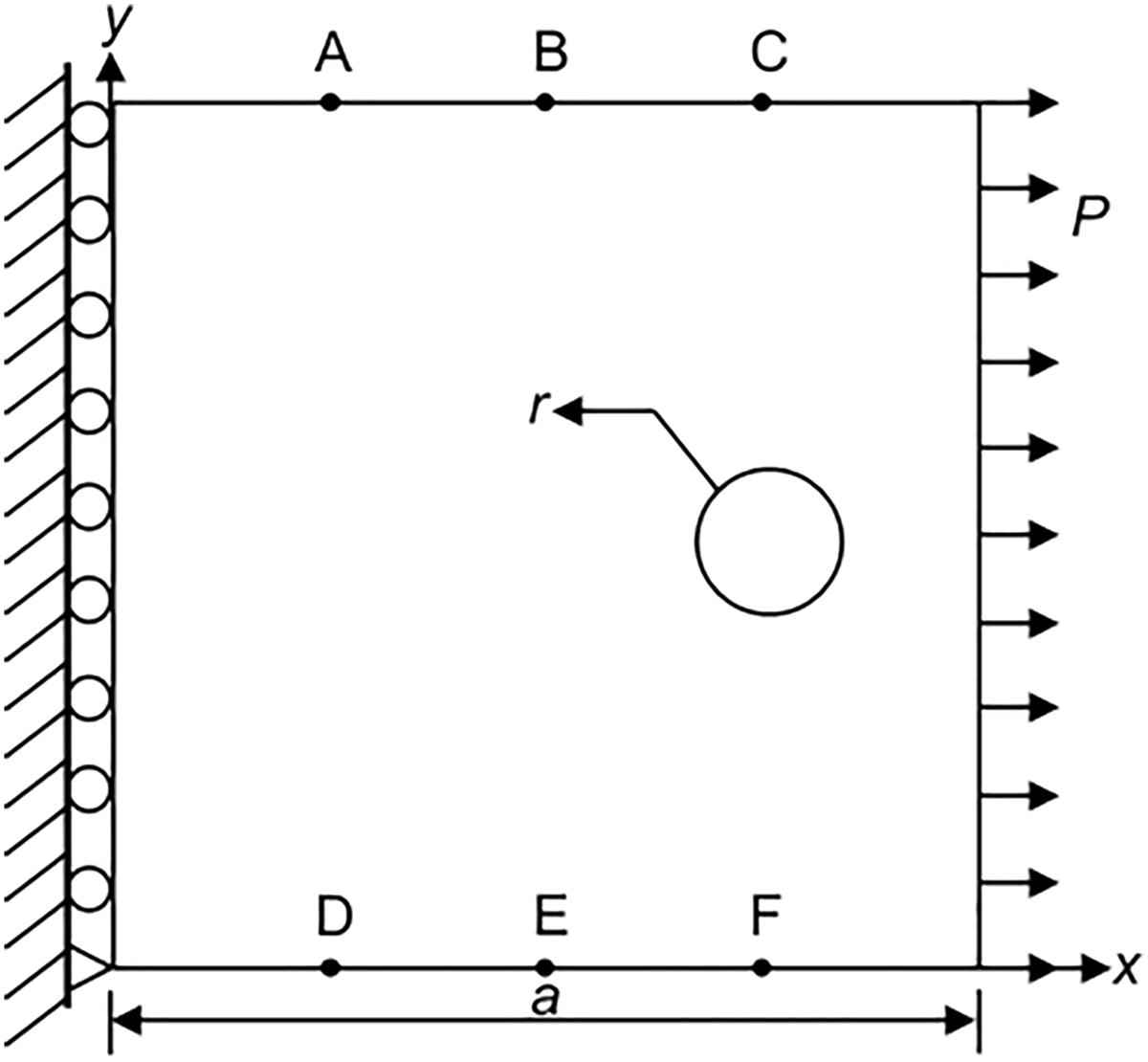
Figure 4: The geometric dimensions of square plate structures with a single flaw

According to previous studies in selecting the number of training set samples and test set samples [17], the position coordinates (x, y) and radius (r) of the hole were randomly varied to generate 6200 sample groups with other parameters of the square plate remaining unchanged. The image-based quadtree SBFEM was used for quadtree mesh generation, and the displacements at the observation points for each sample were calculated sequentially. Each sample group used 12 displacement values as data features and 3 flaw parameters as data labels. Of these, 6000 sample groups were used as the training set to train a single-hidden-layer neural network. Subsequently, 200 sample groups were selected the clean data and input into the inversion model as the test set to analyze the model accuracy. All test samples are generated through the same process to ensure the consistency of data generation logic and avoid verification bias caused by distribution shift.

Verification is performed using the prediction results of 200 sets of clean data and several evaluation indexes are calculated. The true value, predicted value and the relative error δ of a typical set of result data are detailed in Table 2. The statistical evaluation of the MAE, MSE and average relative error δ¯ are also obtained and given. The results show that the predicted results agree well with the true values. Furthermore, the relative errors of the flaw parameters were calculated, and histograms of the relative error distributions for the coordinates and radius are shown in Fig. 5. The 95% confidence intervals for the relative errors were [2.16%, 2.76%] for the x-coordinate, [1.53%, 1.96%] for the y-coordinate, and [1.49%, 1.91%] for the radius (r). From the statistical results, it can be observed that for a single circular hole, the established inversion model can accurately detect flaw information.

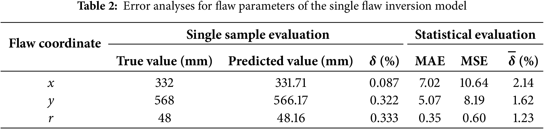
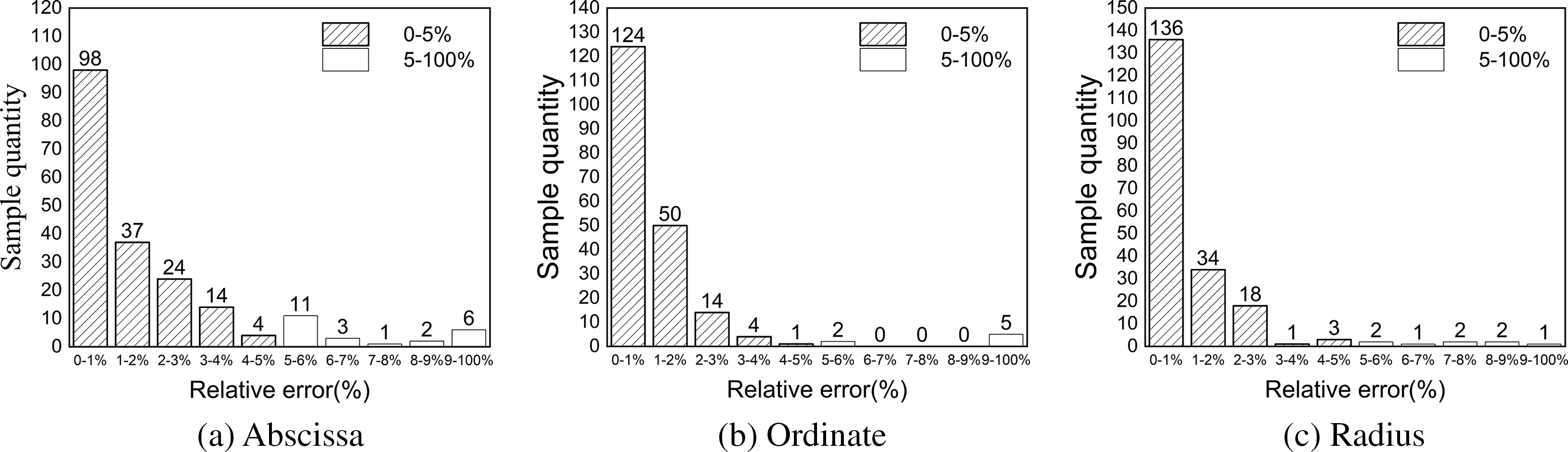
Figure 5: Histograms of relative error distributions. (a) Abscissa. (b) Ordinate. (c) Radius

5.1.1 Influence of Hole Size on Inversion Accuracy

To investigate the influence of hole size on the prediction results of the inversion model, the radius r of the holes to be inverted was set to different proportions of the square plate’s side length, specifically 1/20, 1/24, 1/30, 1/40, 1/50, and 1/60, respectively. For each group, the radius r in the training set was kept constant, and holes were randomly generated within the plate. Each group generated 2200 samples, of which 2000 were used as the training set to train the DNN model, and the remaining 200 served as the test set to analyze the accuracy of each trained model.

Post-processing was performed on the inversion results of 200 test set samples from the six model groups, yielding the MAE values for both the true and inverted coordinates of each model group. The statistical results are presented in Table 3. Additionally, a graph depicting the variation of the overall average relative error of the flaw parameters with respect to radius size is plotted in Fig. 6. Based on the statistical results, the MAE values for the inverted coordinates are all below 6. This indicates that the established single flaw inversion model also exhibits good adaptability in predicting cavity locations. Notably, the circular cavity with a radius-to-plate-side-length ratio of 1/30 exhibits the smallest overall average relative error in the inversion results, with predicted values closest to the true values. However, as the radius range becomes more dispersed, the inversion accuracy tends to decrease.

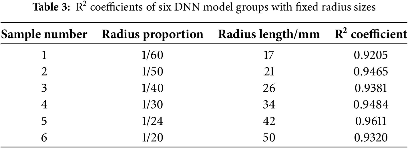
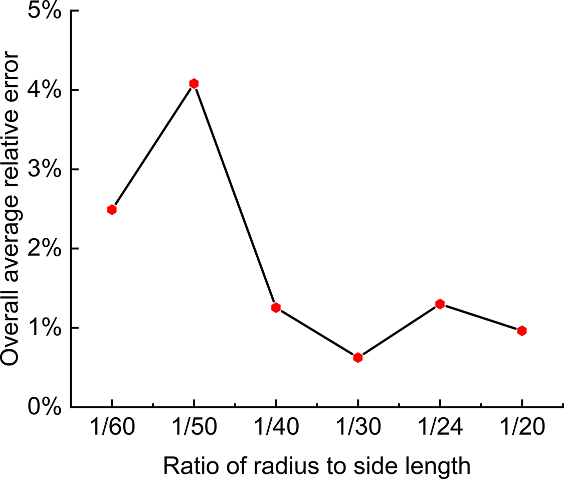
Figure 6: Variation of the overall average relative error of flaw parameters with radius size

5.1.2 Influence of Training Sample Size on Inversion Performance

For the DNN, an increase in the number of training set samples implies improved inversion accuracy; however, it also leads to a corresponding increase in model training time. To investigate the impact of different sample sizes on the model’s inversion capability, this section examines the number of samples in the training set.

The positions (x, y) and radius (r) of holes in a square plate were randomly varied to generate 10,200 sample groups. Each sample was sequentially numbered from 1 to 10,200. Samples numbered 1 to 1000 served as the first training set; those numbered 1 to 2000 formed the second training set; and so on, with samples numbered 1 to 10,000 constituting the tenth training set. The ten training sets were input separately into a DNN model for training. The DNN model used the tanh activation function and had two hidden layers, each with 25 nodes. The training time of each model group was recorded. It should be noted that the training processes of these models were independent of one another.

After training the ten models, 200 reserved test set data were input into each model to obtain the corresponding prediction values (i.e., the inversion values for each model). The number of training set samples significantly affects the model’s inversion accuracy. In this numerical example, the inversion accuracy of the deep learning neural network model tended to stabilize when the sample count ranged from 3000 to 9000. A combined comparison of the inversion result errors of the ten models and their corresponding training times is shown in Fig. 7. It can be observed that as the number of samples increases, the model training time also increases accordingly. Considering both time cost and error accuracy, 3000 data sets are appropriate for training.

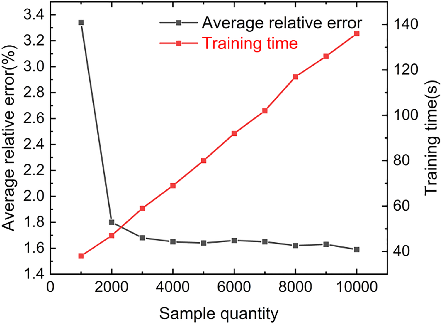
Figure 7: Bivariate plot of sample size impact on inversion errors and training time

5.2 Inversion of Double Circular Flaws

This section explores the applicability of the established flaw inversion model for multi-flaw identification. As shown in Fig. 8, inversion of double flaws are conducted based on the model presented in Section 4. In the numerical example, the dimensions, boundary conditions, material parameters, observation point locations, and loading conditions of the plate with double holes are the same as those described previously. However, the square plate contains two circular hole flaws, with inversion parameters [x1, y1, r1] and [x2, y2, r2].

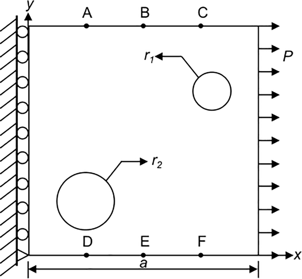
Figure 8: The geometric dimensions of square plate structures with double flaws

In this numerical example, the image quadtree SBFEM was used to calculate the responses at observation points for 6200 random flawed plates. A single-hidden-layer neural network model was trained using 6000 data sets as the training set. After training, 200 data sets were used as the test set to predict the parameters of double flaws. The inversion results are shown in Table 4. The relative errors between the inverted and true values of the double flaws information are within 4%, indicating satisfactory inversion results. The inversion results from the test set were analyzed, and a comparison of the relative errors between the inverted and true flaw parameters is presented in Fig. 9. The prediction results of 200 clean data sets were used for verification. The 95% confidence interval of the error is [3.06%, 3.62%], and the error distribution histogram is shown in Fig. 10. It can be observed that the established inversion model can also accurately detect the location and size of multiple flaws.

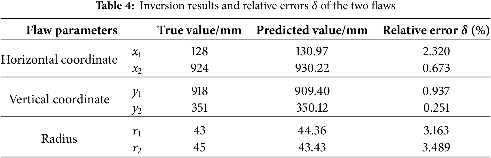
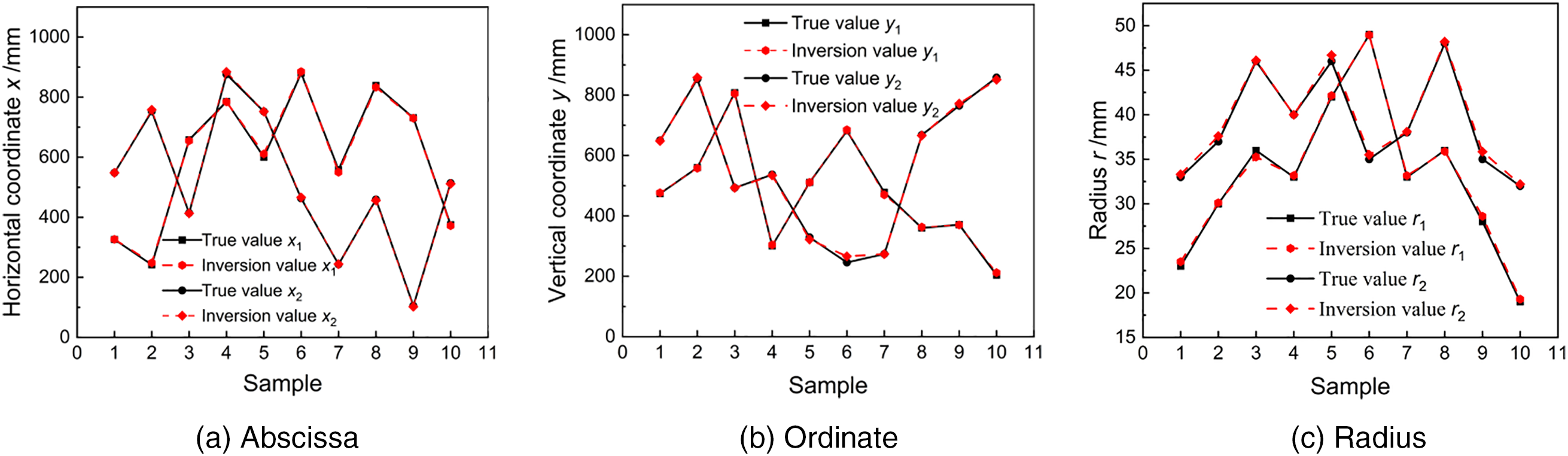
Figure 9: Comparison of inversion results for the double-flaws test set. (a) Abscissa. (b) Ordinate. (c) Radius

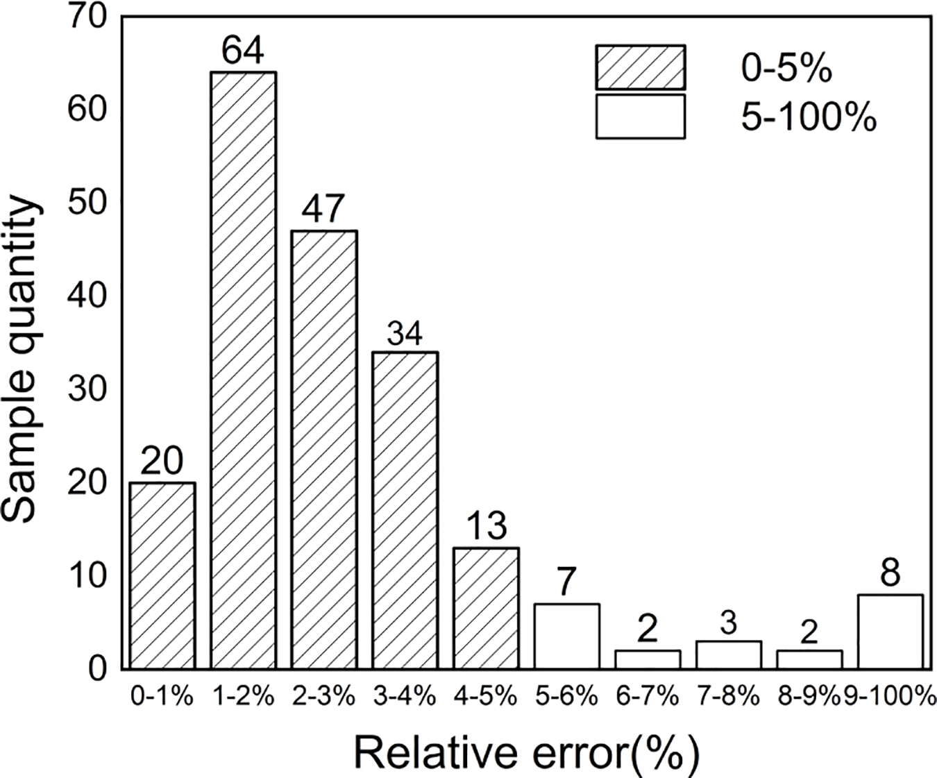
Figure 10: Error distribution histogram for 200 double-flaws samples

5.3 Inversion of Flaw Parameters in Heterogeneous Materials

For the inversion of internal flaws in concrete materials, the material is simplified as a two-phase heterogeneous material composed of polygonal aggregates and cement mortar. CT scanning was performed on laboratory-cast concrete specimens containing gravel aggregates. The aggregate particle gradation and area were statistically analyzed to construct a grayscale image of the mesoscopic model for the heterogeneous concrete structure with polygonal aggregates. The polygonal random aggregate model is a 1000 mm × 1000 mm square plate, with the aggregate elastic modulus E1 = 55 GPa, Poisson’s ratio ν1 = 0.3, cement mortar elastic modulus E2 = 22 GPa, and Poisson’s ratio ν2 = 0.3. The six observation points are positioned as previously described. As shown in Fig. 11, the model’s left end is fixed, and a uniformly distributed load of 25 MPa is applied to the right side. The model also contains a randomly generated circular flaw.

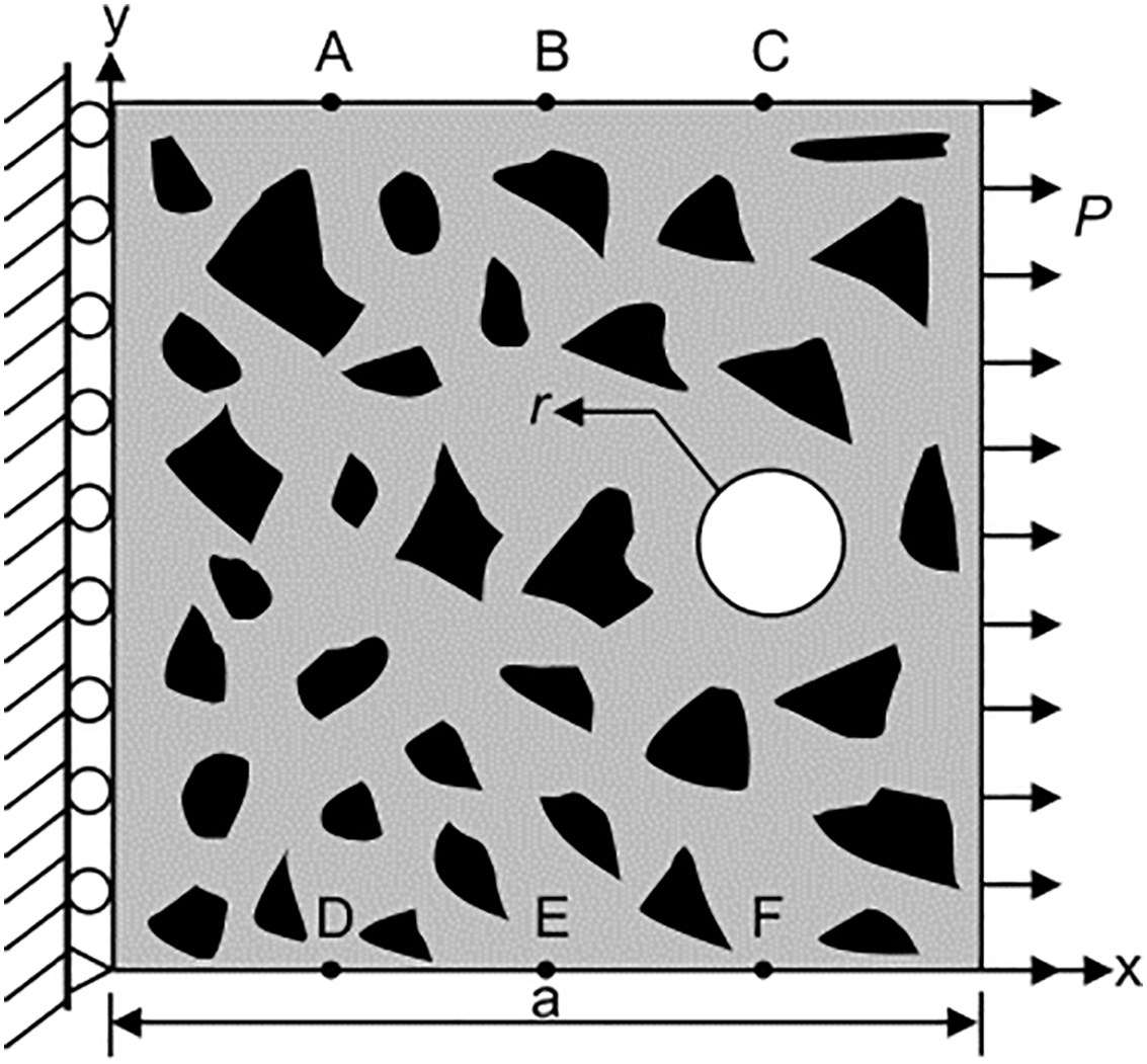
Figure 11: A uniaxial tensile model of heterogeneous concrete structures with flaws

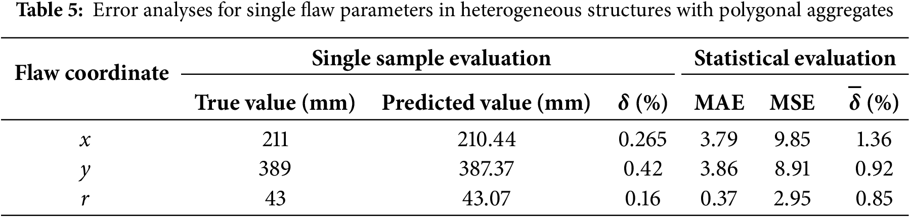
In Heterogeneous Materials, the time to generate the dataset for each group is correspondingly prolonged due to the further complexity of the situation. Considering that the generation time and computational costs, the number of training set groups has a slightly decrease. Numerical calculations were performed using the image quadtree SBFEM. By randomly varying positions, 5200 sample groups were rapidly generated. Herein, 5000 groups were used to train the DNN model, and 200 groups served as the test set to predict the flaw parameters (x, y, r). The error evaluations of inversion results on a typical set are detailed as shown in Table 5. What’s more, the statistical evaluations of the MAE, MSE and average relative error are also obtained and given. The errors between the predicted values and the true values are small. The results show that the predicted results agree well with the true values.

6  Conclusion

(1)   An inversion model suitable for internal structural flaws was established based on the image quadtree SBFEM and DNN algorithm. The sample collection process and data preprocessing methods are presented. Detailed explanations are provided regarding the observation point arrangement scheme, relevant parameters of the DNN, and the establishment process of the flaw inversion model. Based on the model evaluation method, it was determined that when the proposed inversion model uses the tanh activation function and 25 neurons, it can accurately predict structural flaw parameters while controlling time costs.

(2)   The model was validated through several numerical examples. The relative errors between the inversion results and true values are extremely small. For the single flaw, the 95% confidence intervals of the relative error for (x, y, r) are [2.16%, 2.76%], [1.53%, 1.96%] and [1.49%, 1.91%], respectively. The 95% confidence interval of the comprehensive relative error for double flaws is [3.06%, 3.62%]. Average relative errors of (x, y, r) are all less than 1.5% in the inversion of heterogeneous plates. The results demonstrate that the constructed model can accurately identify the locations and sizes of internal flaws in structures.

(3)   A further analysis was conducted on the influence of hole size and sample quantity on the inversion results in the single-flaw inversion model. It was concluded that when the hole radius is 1/30 of the square plate’s side length and the sample quantity is 3000, the established flaw inversion model can achieve the highest preprocessing efficiency while ensuring inversion accuracy.

(4)   This model achieves accurate identification of circular defects in single hole, double holes, and heterogeneous materials based on numerical simulation. By combining the adaptive ability of quadtree grids to irregular boundaries, it can be applied to cover complex defect morphologies by expanding training samples (such as rectangular and crack-like flaws). The applicability of the proposed method would be verified through experiments and other different loading conditions in future studies. Meanwhile, multi-source features such as vibration and temperature can be combined with the mature applications of SBFEM in dynamics, heat conduction and other fields to improve the defect identification ability of the model under complex working conditions. It demonstrates the potential for more complex types of defects and other aspects.

Acknowledgement: Not applicable.

Funding Statement: This research was funded by the National Natural Science Foundation of China (Grant No. 52109152) and the Jiangxi Provincial Natural Science Foundation (Grant Nos. 20242BAB25023 and 20232BAB214086).

Author Contributions: Conceptualization, Hanyu Tao and Tao Fang; Methodology, Hanyu Tao; Software, Dongye Sun; Validation, Wenhu Zhao, Hanyu Tao and Tao Fang; Writing—original draft, Hanyu Tao and Dongye Sun; Writing—review & editing, Wenhu Zhao; Supervision, Dongye Sun and Wenhu Zhao. All authors reviewed the results and approved the final version of the manuscript.

Availability of Data and Materials: Data available on request from the authors.

Ethics Approval: Not applicable.

Conflicts of Interest: The authors declare no conflicts of interest to report regarding the present study.

References

1. Xu X, Ran B, Jiang N, Xu L, Huan P, Zhang X, et al. A systematic review of ultrasonic techniques for defects detection in construction and building materials. Measurement. 2024;226:114181. doi:10.1016/j.measurement.2024.114181. [Google Scholar] [CrossRef]

2. Xue Y, Gao J, Liu J, Shen X, Zhang B, Feng Q. Nondestructive testing of internal defects by ring-laser-excited ultrasonic. Nondestruct Test Eval. 2024;39(8):2277–94. doi:10.1080/10589759.2023.2297081. [Google Scholar] [CrossRef]

3. Kang MS, Kim N, Lee JJ, An YK. Deep learning-based automated underground cavity detection using three-dimensional ground penetrating radar. Struct Health Monit. 2020;19(1):173–85. doi:10.1177/1475921719838081. [Google Scholar] [CrossRef]

4. Hou Z, Zhao W, Yang Y. Identification of railway subgrade defects based on ground penetrating radar. Sci Rep. 2023;13(1):6030. doi:10.1038/s41598-023-33278-w. [Google Scholar] [PubMed] [CrossRef]

5. Chang HL, Ren HT, Wang G, Yang M, Zhu XY. Infrared defect recognition technology for composite materials. Front Phys. 2023;11:1203762. doi:10.3389/fphy.2023.1203762. [Google Scholar] [CrossRef]

6. Kabouri A, Khabbazi A, Youlal H. Applied multiresolution analysis to infrared images for defects detection in materials. NDT E Int. 2017;92(1):38–49. doi:10.1016/j.ndteint.2017.07.014. [Google Scholar] [CrossRef]

7. Segnidi H, Wahid A, Fouaidi M, Kartouni A, Elghorba M. Monitoring damage development in glass fiber/epoxy laminated composites under cyclic shear fatigue loading using acoustic emission. Thin Walled Struct. 2025;215:113524. doi:10.1016/j.tws.2025.113524. [Google Scholar] [CrossRef]

8. Ma S, Li S, Wu C, Zhang X, Zeng Z. Crack detection and damage evaluation of asymmetrical steel-reinforced concrete frame nodes using acoustic emission technology. Nondestruct Test Eval. 2025;40(4):1424–50. doi:10.1080/10589759.2024.2351171. [Google Scholar] [CrossRef]

9. Nishimura N, Kobayashi S. A boundary integral equation method for an inverse problem related to crack detection. Int J Numer Meth Eng. 1991;32(7):1371–87. doi:10.1002/nme.1620320702. [Google Scholar] [CrossRef]

10. Mellings SC, Aliabadi MH. Flaw identification using the boundary element method. Int J Numer Meth Eng. 1995;38(3):399–419. doi:10.1002/nme.1620380304. [Google Scholar] [CrossRef]

11. Ma C, Yu T, Van Lich L, Quoc Bui T. An effective computational approach based on XFEM and a novel three-step detection algorithm for multiple complex flaw clusters. Comput Struct. 2017;193(3):207–25. doi:10.1016/j.compstruc.2017.08.009. [Google Scholar] [CrossRef]

12. Zhao W, Du C, Jiang S. An adaptive multiscale approach for identifying multiple flaws based on XFEM and a discrete artificial fish swarm algorithm. Comput Meth Appl Mech Eng. 2018;339(3):341–57. doi:10.1016/j.cma.2018.04.037. [Google Scholar] [CrossRef]

13. Zhang L, Yang G, Hu D. Identification of voids in structures based on level set method and FEM. Int J Comput Methods. 2018;15(3):1850015. doi:10.1142/s0219876218500159. [Google Scholar] [CrossRef]

14. Ramujee K, Sadula P, Madhu G, Kautish S, Almazyad AS, Xiong G, et al. Prediction of geopolymer concrete compressive strength using convolutional neural networks. Comput Model Eng Sci. 2024;139(2):1455–86. doi:10.32604/cmes.2023.043384. [Google Scholar] [CrossRef]

15. Zarouan M, Mehedi IM, Latif SA, Rana MM. Gradient optimizer algorithm with hybrid deep learning based failure detection and classification in the industrial environment. Comput Model Eng Sci. 2024;138(2):1341–64. doi:10.32604/cmes.2023.030037. [Google Scholar] [CrossRef]

16. Dong X, Taylor CJ, Cootes TF. Defect detection and classification by training a generic convolutional neural network encoder. IEEE Trans Signal Process. 2020;68:6055–69. doi:10.1109/TSP.2020.3031188. [Google Scholar] [CrossRef]

17. Yang Y, Zhou X, Liu Y, Hu Z, Ding F. Wood defect detection based on depth extreme learning machine. Appl Sci. 2020;10(21):7488. doi:10.3390/app10217488. [Google Scholar] [CrossRef]

18. Nguyen-Ngoc L, Nguyen-Huu Q, De Roeck G, Bui-Tien T, Abdel-Wahab M. Deep neural network and evolved optimization algorithm for damage assessment in a truss bridge. Mathematics. 2024;12(15):2300. doi:10.3390/math12152300. [Google Scholar] [CrossRef]

19. Huang X, Peng X, Qin F, Yang Q, Xu B. Damage detection of beam structures using displacement differences and an artificial neural network. Coatings. 2025;15(3):289. doi:10.3390/coatings15030289. [Google Scholar] [CrossRef]

20. Song C, Wolf JP. The scaled boundary finite-element method—alias consistent infinitesimal finite-element cell method—for elastodynamics. Comput Meth Appl Mech Eng. 1997;147(3–4):329–55. doi:10.1016/S0045-7825(97)00021-2. [Google Scholar] [CrossRef]

21. Qu Y, Eisenträger S, Zhang Z, Zhang L, Song C. Development of a fully automatic damage simulation framework for quasi-brittle materials. Eng Anal Bound Elem. 2023;157:578–95. doi:10.1016/j.enganabound.2023.10.004. [Google Scholar] [CrossRef]

22. Su R, Tangaramvong S, Song C. Automatic image-based SBFE-BESO approach for topology structural optimization. Int J Mech Sci. 2024;263:108773. doi:10.1016/j.ijmecsci.2023.108773. [Google Scholar] [CrossRef]

23. Thananjayan P, Natarajan S, Ooi ET, Ramu P. Scaled boundary finite element based two-level learning approach for structural flaw identification. Eng Anal Bound Elem. 2024;166:24. doi:10.1016/j.enganabound.2024.105855. [Google Scholar] [CrossRef]

24. Thananjayan P, Ramu P, Natarajan S. SBFEM and Bayesian inference for efficient multiple flaw detection in structures. Eng Anal Bound Elem. 2023;155:226–50. doi:10.1016/j.enganabound.2023.06.001. [Google Scholar] [CrossRef]

25. Shen X, Du C, Jiang S, Sun L, Chen L. Enhancing deep neural networks for multivariate uncertainty analysis of cracked structures by POD-RBF. Theor Appl Fract Mech. 2023;125:103925. doi:10.1016/j.tafmec.2023.103925. [Google Scholar] [CrossRef]

26. Song C, Ooi ET, Natarajan S. A review of the scaled boundary finite element method for two-dimensional linear elastic fracture mechanics. Eng Fract Mech. 2018;187:45–73. doi:10.1016/j.engfracmech.2017.10.016. [Google Scholar] [CrossRef]

27. Ooi ET, Natarajan S, Song C, Ooi EH. Dynamic fracture simulations using the scaled boundary finite element method on hybrid polygon–quadtree meshes. Int J Impact Eng. 2016;90:154–64. doi:10.1016/j.ijimpeng.2015.10.016. [Google Scholar] [CrossRef]

28. Tabarraei A, Sukumar N. Adaptive computations using material forces and residual-based error estimators on quadtree meshes. Comput Meth Appl Mech Eng. 2007;196(25–28):2657–80. doi:10.1016/j.cma.2007.01.016. [Google Scholar] [CrossRef]

29. Krysl P, Grinspun E, Schröder P. Natural hierarchical refinement for finite element methods. Int J Numer Meth Eng. 2003;56(8):1109–24. doi:10.1002/nme.601. [Google Scholar] [CrossRef]

30. Jiang S, Wan C, Sun L, Du C. Flaw classification and detection in thin-plate structures based on scaled boundary finite element method and deep learning. Int J Numer Meth Eng. 2022;123(19):4674–701. doi:10.1002/nme.7051. [Google Scholar] [CrossRef]

31. Li J, Liu J, Lin G. Dynamic interaction numerical models in the time domain based on the high performance scaled boundary finite element method. Earthq Eng Eng Vib. 2013;12(4):541–6. doi:10.1007/s11803-013-0195-8. [Google Scholar] [CrossRef]