
 Submit a Paper
 Propose a Special lssue
 Open Access
ARTICLE
Predicting the Compressive Strength of Self-Consolidating Concrete Using Machine Learning and Conformal Inference
1 Department of Civil and Building Engineering, Université de Sherbrooke, Sherbrooke, QC J1K 2R1, Canada
2 Department of Architecture, Canadian University Dubai, Dubai, P.O. Box 117781, United Arab Emirates
3 Department of Mathematical and Statistical Sciences, University of Colorado Denver, Denver, CO 80204, USA
* Corresponding Author: Masoud Hosseinpoor. Email:
Computer Modeling in Engineering & Sciences 2025, 145(3), 3309-3347. https://doi.org/10.32604/cmes.2025.072271
Received 23 August 2025; Accepted 07 November 2025; Issue published 23 December 2025
 View Full Text
 Download PDF
Abstract
Self-consolidating concrete (SCC) is an important innovation in concrete technology due to its superior properties. However, predicting its compressive strength remains challenging due to variability in its composition and uncertainties in prediction outcomes. This study combines machine learning (ML) models with conformal prediction (CP) to address these issues, offering prediction intervals that quantify uncertainty and reliability. A dataset of over 3000 samples with 17 input variables was used to train four ensemble methods, including Random Forest (RF), Gradient Boosting Regressor (GBR), Extreme gradient boosting (XGBoost), and light gradient boosting machine (LGBM), along with CP techniques, including cross-validation plus (CV+) and conformalized quantile regression (CQR) methods. Results demonstrate that LGBM and XGBoost outperform RF, improving R2 by 4.5% and 5.7% and reducing Root-mean-square Error (RMSE) by 24.6% and 24.8%, respectively. While CV+ yielded narrower but constant intervals, CV+_Gamma and CQR provided adaptive intervals, highlighting trade-offs among precision, adaptability, and coverage reliability. The integration of CP offers a robust framework for uncertainty quantification in SCC strength prediction and marks a significant step forward in ML applications for concrete research.Keywords
Over the past two decades, concrete has evolved from a simple mixture of cement, aggregate, and water into a highly engineered material incorporating a variety of new advanced components. Among these advancements, self-consolidating concrete (SCC) is known as one of the most promising innovations due to its superior performance compared to traditional concrete [1]. SCC is highly deformable and has good resistance to segregation; it flows under its own weight through congested reinforcement without the need for mechanical vibration. SCC has now become a material that is being used around the world with many different types of applications and structural configurations [2].
Determining the compressive strength of concrete is essential for the structural design of buildings and infrastructure. In practice, the compressive strength is assessed through laboratory testing of standard specimens after a designated curing period under controlled conditions. While reliable, this conventional approach is time-consuming, labor-intensive, and costly [3]. To overcome these limitations, the application of machine learning (ML), a branch of artificial intelligence (AI), has recently emerged as a transformative and innovative approach in the construction industry, leading to enhanced efficiency, greater predictive accuracy, and the potential of data-driven advancements [4].
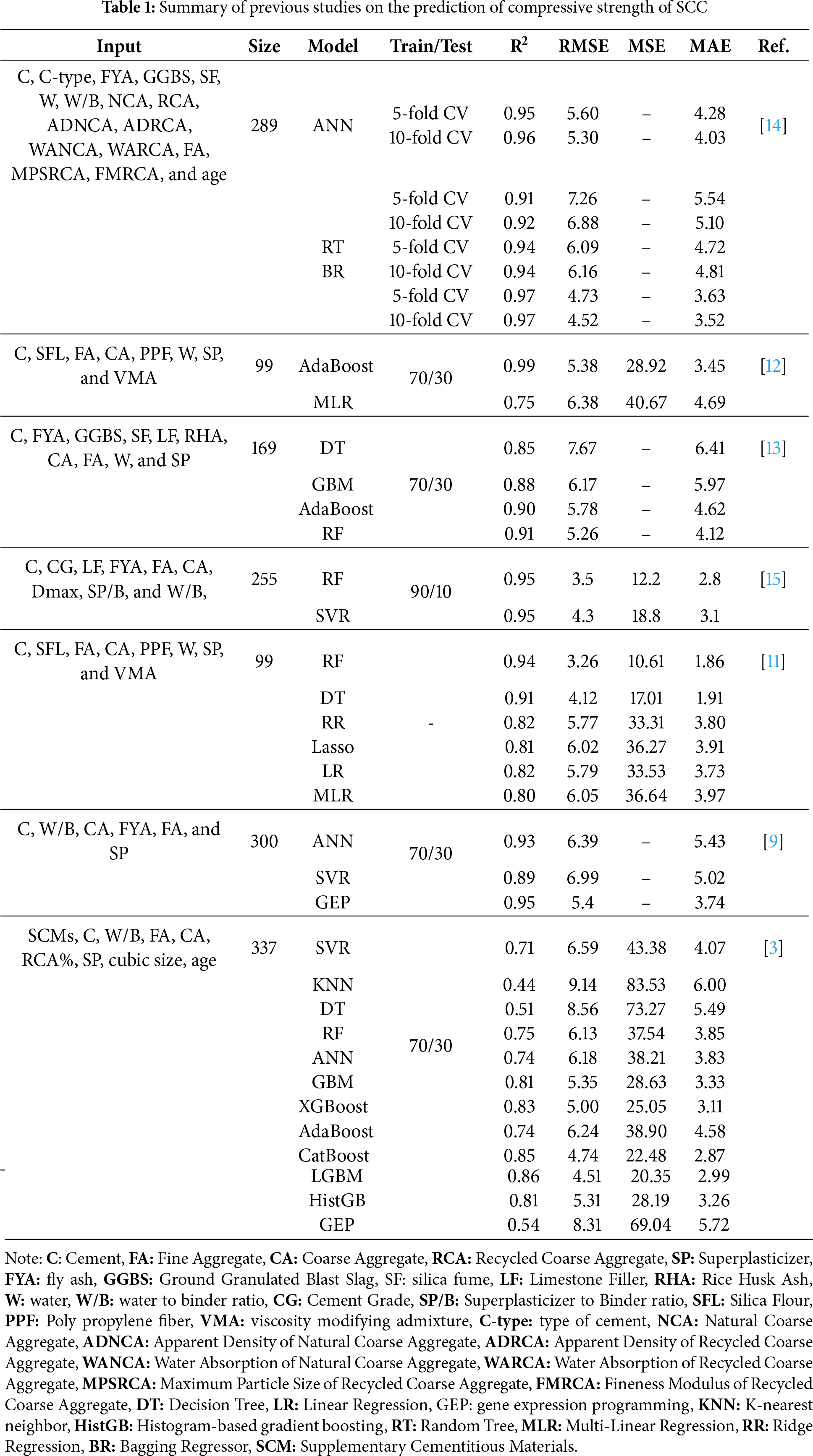
Numerous studies have successfully used ML techniques to predict the compressive strength of concrete. For instance, Shafighfard et al. [5] demonstrated that stacked ML models combining support vector regressor (SVR), random forest (RF), extra tree regression (ETR), gradient boosting regressor (GBR), and K-nearest neighbors (KNN) significantly improved the prediction accuracy for steel fiber-reinforced concrete compared to an artificial neural network (ANN) model. Similarly, a recent study reported that integrating active learning with stacked ensembles can significantly enhance the predictive performance of ML models for estimating the compressive strength of alkali-activated ultra-high-performance concrete. In this approach, base learners are iteratively retrained on selectively labeled, high-information samples identified through active learning strategies, enabling the ensemble to capture complex patterns in the data [6]. Golafshani et al. [7] applied eight different ensemble models to predict the compressive strength of geopolymer recycled aggregate concrete using a synthetically generated dataset. Among these, the extreme gradient boosting machine (XGBoost) model achieved the highest test accuracy, outperforming the other models. Moreover, a recent study has shown that coupling tree-based learners with metaheuristic optimization algorithms, such as integrating the Grey Wolf Optimizer (GWO) with RF and XGBoost, can further enhance predictive performance [8]. Farooq et al. [9] investigated the use of ANN, SVR, and gene expression programming (GEP) to predict the compressive strength of SCC incorporating fly ash. All three models exhibited good predictive capability, with GEP outperforming both ANN and SVR in terms of accuracy and error. Kumar et al. [10] applied five different ML models to a dataset of 240 samples to predict the compressive strength of high-volume fly ash SCC. Their findings demonstrated that all models could accurately predict the strength, with RF achieving the highest performance. Similarly, another study predicted the compressive strength of SCC containing recycled coarse aggregate, based on 44 data samples, where GBR achieved an accuracy of 0.96 [4]. Furthermore, Huang et al. [3] examined 12 different ML models to predict the compressive strength of SCC using 337 data samples. The findings revealed that the categorical boosting algorithm (CatBoost) and light gradient boosting machine (LGBM) models generally outperformed the others, offering higher accuracy and lower error rates. Additionally, a laboratory dataset consisting of 99 SCC samples was used for prediction, where the RF model was able to accurately predict the compressive strength [11]. Although a simple train–test split often produces high accuracy, subsequent k-fold cross-validation revealed substantial variability between folds, indicating limited model generalizability [12,13]. Table 1 summarizes the main findings of previous studies on ML-based prediction of SCC compressive strength.
Although ML models have shown great success in making point predictions (mean estimates for regression), they do not provide insights into the uncertainties or the reliability of their predictions. This limitation becomes highly noticeable if the dataset contains noise and outliers, or if the outcomes are subjected to some levels of intrinsic randomness. Providing insight into the uncertainty associated with point estimates would allow for more informed and confident decision-making. One approach to quantifying the uncertainty in ML models is to provide prediction intervals instead of just point predictions [16,17]. Prediction intervals convey the reliability of a ML model’s predictive performance, which is crucial for guiding decision-making and enhancing trust in ML [18].
The Bayesian network is one such approach, providing a robust framework for uncertainty analysis and probabilistic reasoning [19]. For instance, in a study, a Bayesian inference method was applied to predict the strength of sustainable geomaterials, highlighting the effectiveness of this approach in quantifying prediction uncertainty. The study showed that by employing credible intervals (CIs), the Bayesian model could provide a range of plausible values for the predicted material strength, thus reducing uncertainty in the estimates. During validation, the model successfully captured 93.18% of the observed values within the 85% credible intervals, indicating a high level of confidence in its predictions [20]. Furthermore, a multi-level Bayesian framework was also utilized to quantify and differentiate the various sources of uncertainty in the calibration of a cracked hinge model for fiber-reinforced concrete (FRC), demonstrating its effectiveness in directly quantifying inherent parameter variability stemming from material heterogeneity [21]. Despite these advantages, Bayesian methods require the specification of prior distributions, which can be challenging when prior knowledge is either unavailable or uncertain. The selection of priors can significantly impact the results, and an improper choice may lead to biased outcomes [22].
Unlike Bayesian approach, conformal prediction (CP) does not require explicit assumptions about the underlying data distribution, making it robust even in complex real-world applications where the distribution is unknown. In other words, CP is a powerful, distribution-free method for constructing prediction intervals or sets that provide finite-sample coverage guarantees, making it a robust tool for uncertainty quantification in ML. CP operates on the principle of exchangeability, meaning the order in which we receive the data does not affect the model’s predictions, a less restrictive assumption than requiring independently and identically distributed samples. This makes CP highly flexible and applicable across a range of ML models, such as support vector machines (SVM), decision trees (DTs), boosting algorithms, and neural networks.
The primary objective of CP is to create prediction intervals that contain the true target value within a specified coverage level (e.g., 95%). To achieve this, CP divides the data into two sets: a training set, used to build the model, and a calibration set, used to compute nonconformity score. Nonconformity score quantifies how unusual or “nonconforming” a data point is compared to the rest of the data. For a regression problem, a common nonconformity measure is the absolute error between the predicted and actual values as expressed in Eq. (1) [18]:
where
When a new data point is introduced, the model generates a prediction and computes its nonconformity score, which is compared to the threshold. The prediction interval is constructed to include all potential target values that yield nonconformity scores below this threshold. In regression tasks, the resulting prediction interval for a new input xnew takes the following form [18]:
where
The method’s flexibility and distribution-free nature make CP particularly attractive. It provides finite-sample guarantees, ensuring that its prediction intervals will contain the true value with the specified confidence level, even in small datasets [17,18,23].
CP has been successfully applied across a wide range of fields, demonstrating its adaptability in providing reliable uncertainty estimates. For instance, in the medical domain, Nouretdinov et al. [24] applied Transductive Conformal Predictors (TCP) to MRI-based diagnostic and prognostic markers in depression. Their study demonstrated that TCP provided confidence measures for predictions in psychiatric diagnosis, achieving accuracy comparable to traditional ML methods like SVM, while also offering a valid measure of prediction reliability. Moreover, in the drug discovery process, CP has been integrated into QSAR modeling to assess the solubility and toxicity of chemical compounds [25]. In addition, in software engineering, Papadopoulos et al. [26] applied CP to software effort estimation, utilizing ridge regression to generate predictive intervals for project effort estimations. This approach improved confidence in project management decisions by providing reliable prediction intervals. Similarly, CP has been employed in earth observation to quantify uncertainty in ML models applied to satellite data, aiding in more dependable environmental monitoring and analysis [27]. Furthermore, in structural engineering, CP has been adapted to improve seismic response prediction by introducing data-dependent weights for calculating nonconformity scores. This method provided more precise prediction intervals for high-confidence predictions, surpassing traditional methods like Gaussian Process Regression (GPR) [17].
While CP has been applied in various scientific fields and even tested on publicly available datasets, including the concrete dataset from the UCI repository (Refs. [28–31]), these studies have not addressed the challenges specific to concrete technology. The performance of hardened concrete is influenced by numerous interacting parameters. Although curing can be rigorously controlled in laboratory settings, field variables such as temperature, relative humidity, rainfall, and wind fluctuate during the placement and curing. At the material level, parameters including the size and fineness of cement particles, the reactive content and surface area of SCMs, chemical composition, and particle size distribution (PSD) play a critical role and can vary considerably depending on geographic origin and source [32]. Because the dataset used in this study includes experimental results from several countries with differing material characteristics, even small variations in these parameters can alter hydrations kinetics and, consequently, compressive strength. In this context, uncertainty quantification reflects the extent to which the true compressive strength may deviate from model’s estimate under different materials and environmental conditions. Rather than providing a single deterministic value, CP offers a prediction interval at a selected confidence level (e.g., 90%–95%). This ensures that the true value lies within the predicted interval at the specified frequency, enabling risk-aware and more reliable decision-making. To the best of authors’ knowledge, no research has specifically applied CP to tackle uncertainty estimation in SCC, where managing variability is critical. This study takes the first step toward bridging this gap by investigating how CP can provide more reliable and trustworthy predictions in the field of concrete technology.
To this end, the present study aims to integrate uncertainty quantification through CP alongside traditional point prediction for estimating the compressive strength of SCC. To the best of our knowledge, this is the first study that systematically evaluates and compares multiple CP variants, namely cross-validation plus (CV+), CV+_Gamma, and Conformalized Quantile Regression (CQR), within the context of SCC. The performance of these approaches is assessed at different target coverage levels (90%, 85%, and 80%), providing practical insights into the adaptiveness and reliability of the generated prediction intervals. The comparative analysis highlights the advantages of adaptive CP methods, such as CV+_Gamma, in producing more informative and statistically valid uncertainty estimates, which are essential for informed decision-making in concrete mix design and quality control. The study is supported by the largest and most comprehensive dataset on SCC compressive strength to date, comprising 3005 data points. By explicitly addressing the inherent uncertainties associated with concrete behavior, this study not only enhances prediction accuracy but also provides a more reliable and interpretable framework for compressive strength forecasting in concrete technology. The study is supported by the largest and most comprehensive dataset on SCC compressive strength to date, comprising 3005 data points. By explicitly addressing the inherent uncertainties associated with concrete behavior, this study not only enhances prediction accuracy but also provides a more reliable and interpretable framework for compressive strength forecasting in concrete technology.
To achieve these objectives, the paper is structured, as follows: Section 2 outlines the methodology employed in this study, including data preparation steps, model explanation, and CP for uncertainty quantification. Given the success of ensemble tree models in capturing complex relationships within data, this study focuses on four ensemble methods, RF, GBR, XGBoost, and LGBM due to their proven efficacy in similar tasks. Sections 3 and 4 presents the results of point prediction, SHapley additive exPlanations (SHAP), and conformal prediction to evaluate the reliability and robustness of the predictive models. Section 5 draws conclusions and recommendations for future research.
Fig. 1 illustrates the schematic representation of the current study. The process begins with data collection, followed by exploratory data analysis (EDA) to identify any anomalies or outliers. Next, the data undergoes processing to address missing values and outliers. Once the data is preprocessed, it is utilized for modeling. A 5-fold cross-validation approach will be applied for hyperparameter tuning and model training. After selecting the optimized model, it will be tested on unseen data samples. The final step involves uncertainty estimation using the CP method. Further details of each step are outlined in Fig. 1.
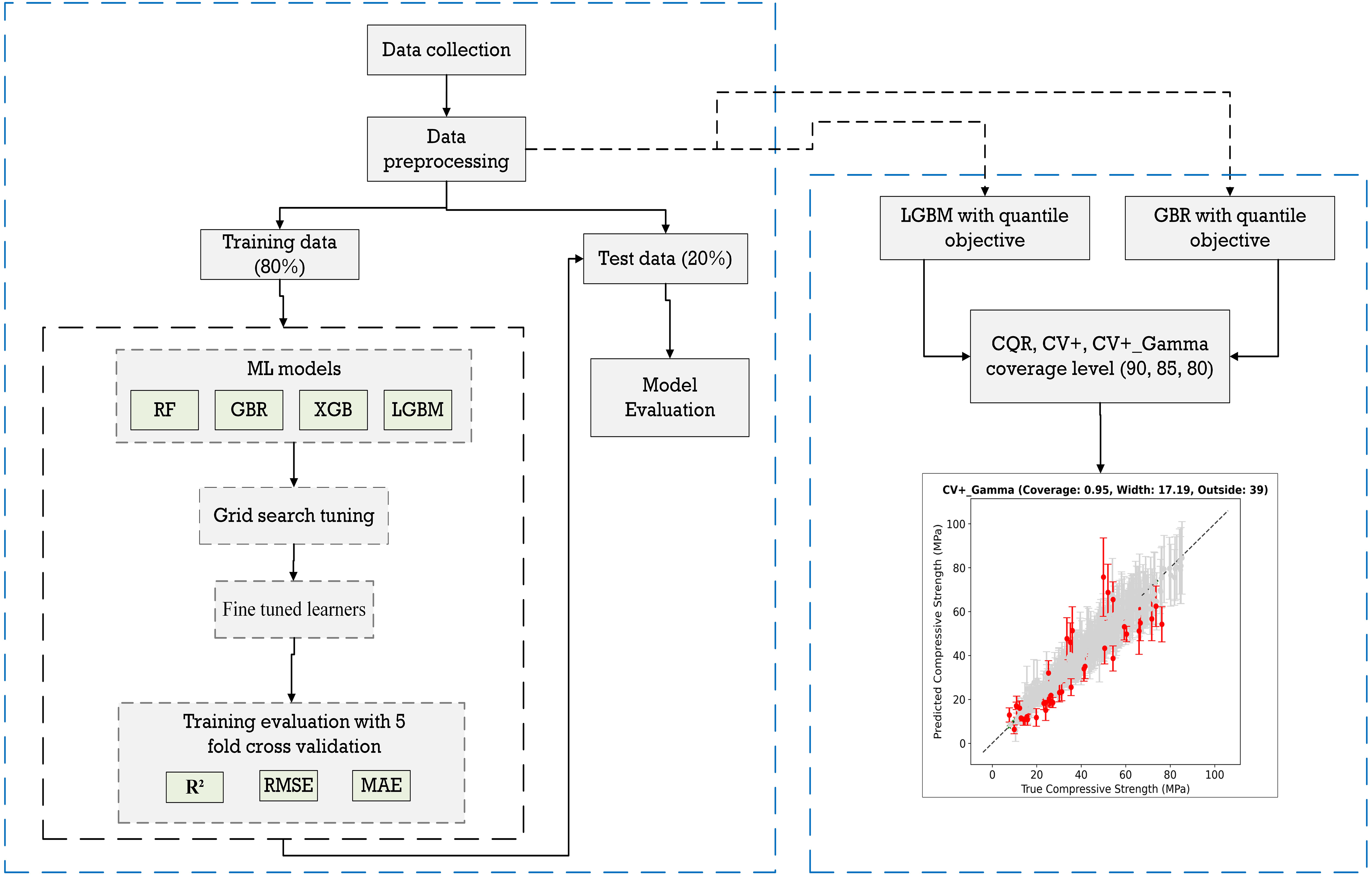
Figure 1: Schematic representation of the study
The size of the dataset used for training plays a crucial role in model performance, as smaller datasets are prone to overfitting. Overfitting occurs when a learning algorithm fits the training data well but cannot maintain performance when evaluated on unseen test data. This over-reliance on the training set limits the model’s ability to generalize, resulting in reduced accuracy and inconsistent results when applied to new unseen data [33]. To address this issue and enable accurate prediction of SCC compressive strength, a comprehensive dataset comprising 3005 data points was collected from 64 journal articles, 2 conference papers, and 16 theses conducted at the Université de Sherbrooke [34–115]. The binder in SCC is commonly produced by combining ordinary Portland cement (OPC) with supplementary cementitious materials (SCMs). In this research, only studies have been considered that contain slag, fly ash, silica fume, and metakaolin as SCMs. Unlike OPC, which has a relatively stable chemical composition, the properties of SCMs can vary significantly due to their natural origins or their role as by-products from other industries. This variability can greatly impact the performance of concrete binders and poses challenges when trying to apply mix designs across different regions. To address this variability and improve the general applicability of mix design processes, Xie and Visintin [116] proposed a unified method for incorporating SCMs into concrete. This method introduces a reactivity index, which considers the chemical composition of the binder. By identifying the key oxides that influence binder reactivity, the reactivity of a cementitious material can be quantified using reactivity moduli. To this end, three moduli, including reactivity modulus (RM), hydraulic modulus (HM), and silica modulus (SM), are calculated using Eqs. (3)–(5) [116].
Finally, the overall reactivity of a blended binder is determined by calculating the weighted average of these moduli, which are subsequently used as input features in predictive models. The RM, SM, and HM are computed according to the details reported in the study by Xie et al. [117].
A total of 17 input variables were analyzed in this study, including contents of cement (kg/m3), slag (kg/m3), fly ash (kg/m3), silica fume (kg/m3), metakaolin (kg/m3), filler (kg/m3), admixture (kg/m3), fine aggregate (kg/m3), coarse aggregate (kg/m3), and water (kg/m3), as well as the water-to-binder ratio (W/B), fine aggregate-to-total aggregate ratio (FA/Tagg), maximum aggregate size (Dmax), age, RM, SM, and HM. These features were selected based on their known effect on the compressive strength of SCC. SCMs, such as fly ash, silica fume, and metakaolin affect both the rate and extent of C–S–H formation. Fly ash generally reduces early-age strength due to its dilution effect and slower pozzolanic reaction, whereas silica fume, typically incorporated at 5%–10%, enhances strength through its high reactivity, micro-filler properties, and nucleation effects. Similarly, metakaolin contributes to strength development through accelerated hydration and pozzolanic reactions, with reported strength gains up to approximately 27%, depending on dosage and W/B. The W/B ratio governs the gel-to-space ratio, where higher values consistently lead to reduced strength. High-range water-reducing admixtures improve particle dispersion and decrease the effective water demand, allowing lower W/B while maintaining adequate workability. Limestone filler enhances particle packing and provides additional nucleation sites, which can modestly accelerate hydration and increase strength at moderate dosages. Aggregate grading (fine vs. coarse), captured by FA/Tagg and Dmax influences packing, paste demand, and the interfacial transition zone (ITZ), all of which affect the resulting strength. Finally, the oxide-based indices (RM, SM, HM) reflect the binder’s chemical composition and its potential C–S–H yield, thereby providing insight into the overall strength development of SCC [56,79,80].
To maintain consistency across data samples, filler was excluded from the calculation of the binder for the W/B ratio, as it is not considered in this calculation in many studies. Additionally, the chemical properties of the filler were not considered in RM, SM, and HM calculations, as its chemical composition is often not reported in most studies. All strength measurements recorded for cubic specimens were converted to their equivalent cylindrical values [118]. A detailed statistical analysis of the input and output variables is presented in Table 2.

EDA was conducted, and visualizations such as distribution plots and box plots were generated (Figs. 2 and 3) to provide insights into the data distribution and detect outliers. Outliers, data points that deviate significantly from most observations, can negatively impact the performance of ML models, leading to inaccurate predictions on new data. Therefore, handling outliers is crucial for building robust and reliable models [119]. In this study, outliers were treated using a percentile-based trimming approach, where data points below the 1st percentile and above the 99th percentile were removed to minimize the impact of extreme values on model training. Following this step, the final dataset used for model development comprised 2341 samples. To ensure comparability among features and improve the convergence of the ML algorithm, Min-Max scaling was applied to normalize all variables within the range of (0, 1). This transformation was performed according to Eq. (6):
where X is the original value, Xmin and Xmax are the minimum and maximum values of the feature, and Xscaled is the normalized value. Min-Max scaling ensures that all features contribute proportionally to the ML models by transforming them into a common range, thereby preventing features with larger magnitudes from dominating the learning process and improving overall model performance. To prevent data leakage, scaling was performed after the dataset was divided into training and test sets.
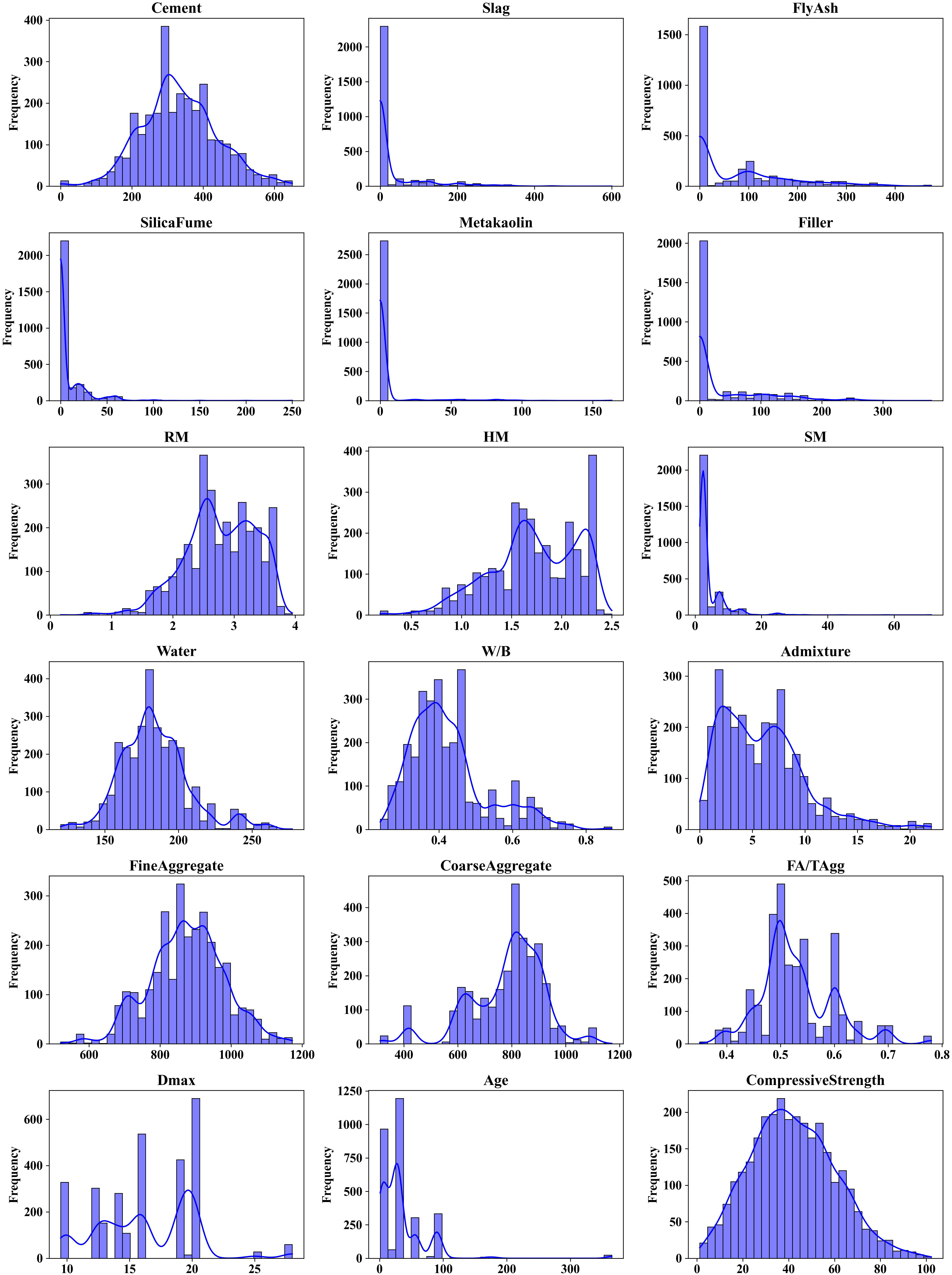
Figure 2: Histogram plot of input variables and output
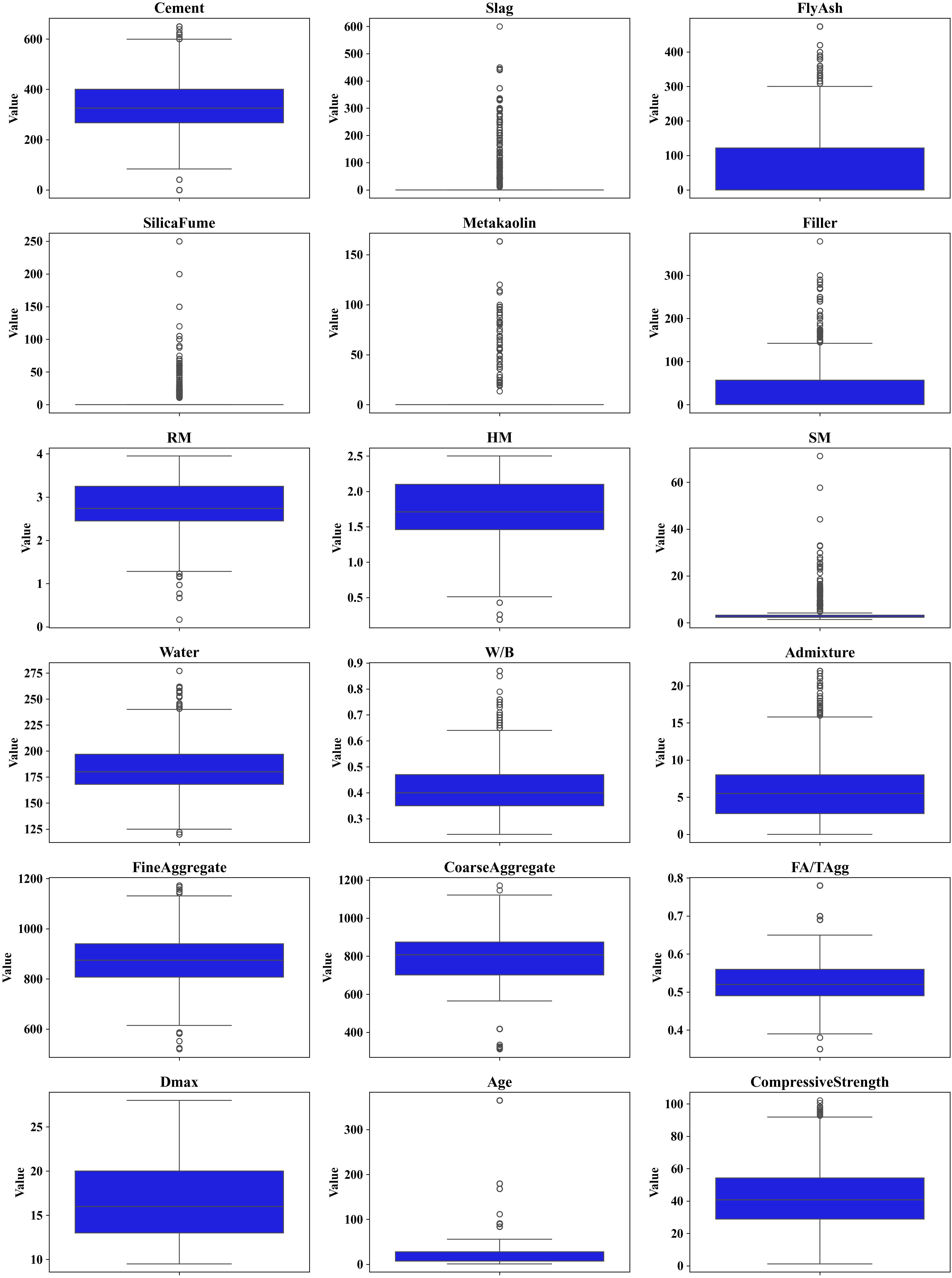
Figure 3: Box plot of input variables and output
To better understand the relationships among input features and their relevance to the target variable, a Pearson correlation heatmap was generated (Fig. 4). As shown, several input variables exhibited moderate correlations with compressive strength. Notably, cement content (r = 0.33), admixture dosage (r = 0.34), and age (r = 0.50) demonstrated high positive correlations with compressive strength, reflecting their significant influence in improving the mechanical performance of SCC. On the other hand, W/B displayed a negative correlation (r = −0.43), consistent with the well-established knowledge that higher W/B generally led to reduced strength. Strong inter-feature correlations were also observed, such as between RM and HM (r = 0.96) and between coarse aggregate and FA/TAgg (r = −0.94), indicating potential redundancy among some input variables. However, since Pearson correlation captures only linear relationships, it may not fully reflect the complex, nonlinear interactions among features. Therefore, additional feature selection and importance analysis methods, such as SHAP values and Partial Dependence Plot (PDP), were employed to provide a more comprehensive understanding of the relative contributions of each input feature.
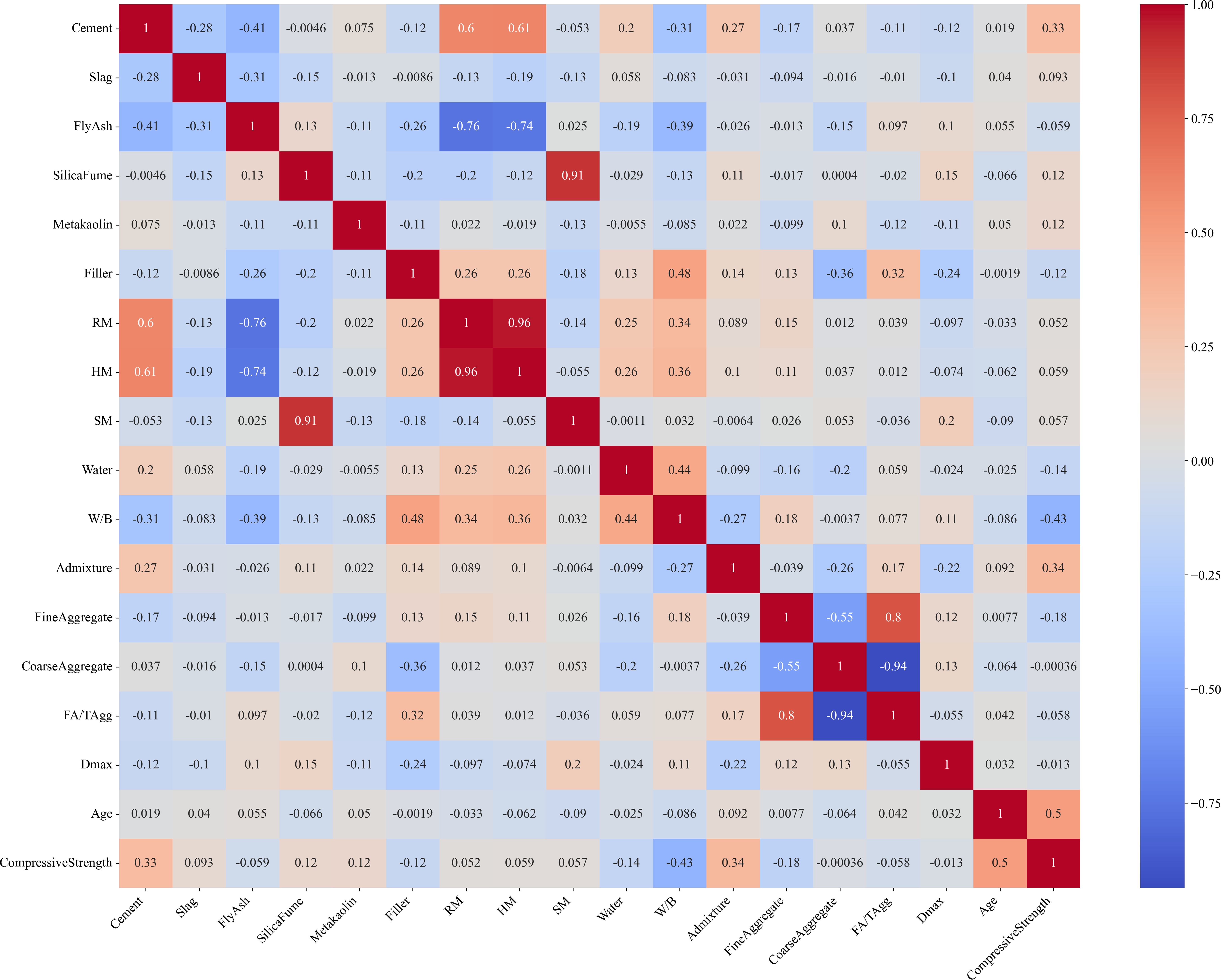
Figure 4: Heatmap plot of the investigated SCC dataset
Feature selection plays a critical role in developing accurate and interpretable ML models, particularly for complex, multi-variable systems such as concrete mix design. Identifying the most relevant input parameters not only improves model performance but also deepens the understanding of the physical mechanisms governing compressive strength. In this study, both SHAP and PDP were used to evaluate feature importance and guide the final input selection process.
SHAP values were calculated for two representative models, LGBM and RF, to quantify the contribution of each feature to SCC compressive strength predictions (Fig. 5). The results consistently highlight age, W/B, admixture dosage, cement content, and Dmax as the most influential variables. Minor differences in features ranking were observed between models, an expected outcome given their distinct learning strategy. For example, RM, silica fume, and coarse aggregate exhibited varying importance across models. To ensure robustness and generalizability, all features were retained in the final modeling phase, preventing the exclusion of variables that may exhibit non-linear, or interaction effects not captured by a single model.
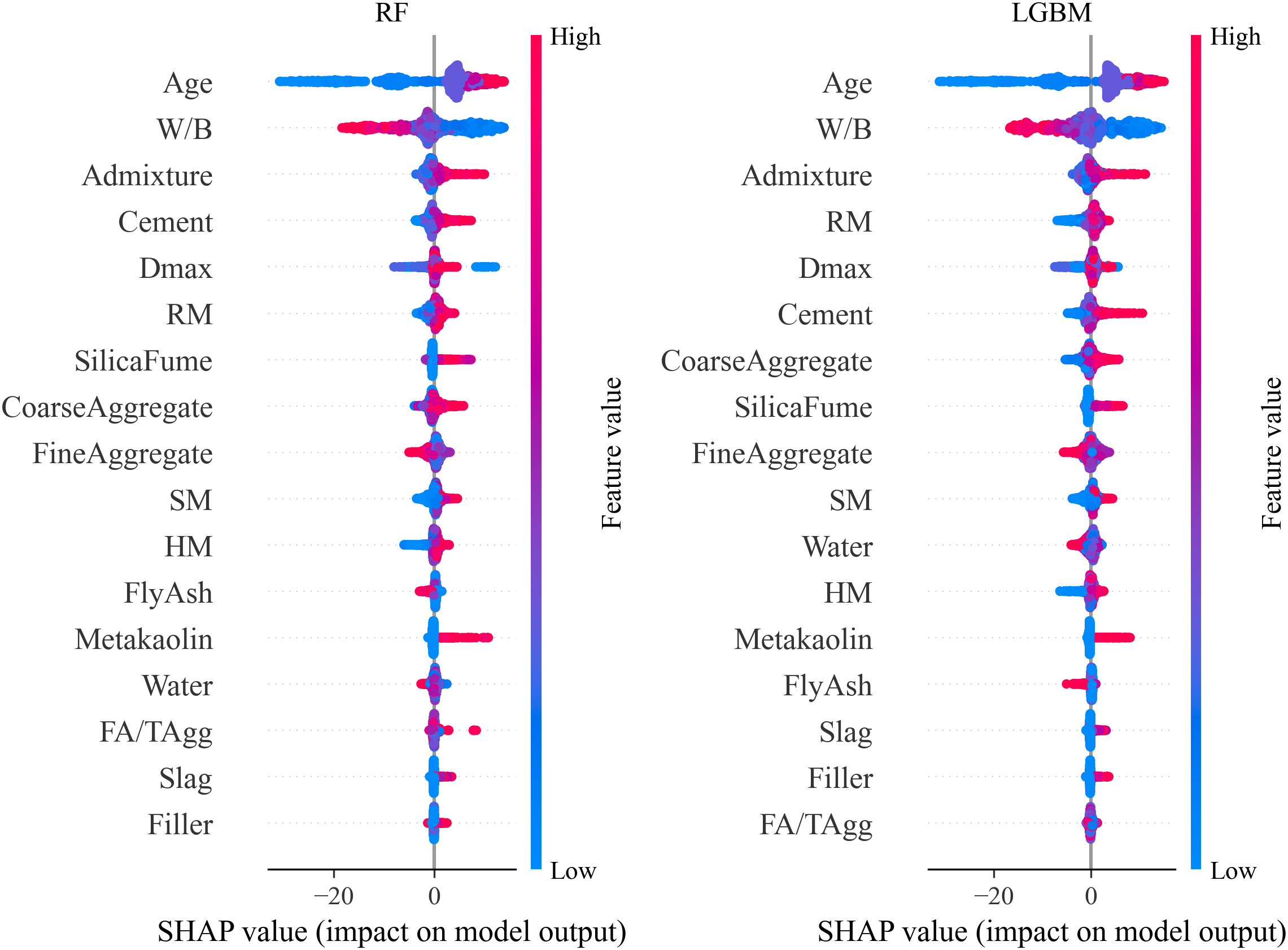
Figure 5: SHAP plot for feature selection
Complementary PDP analyses (Fig. 6) were conducted to illustrate the marginal effect of each feature on predicted strength. While certain parameters, such as slag, fly ash, and FA/Tagg, display relatively flat PDP curves, suggesting a limited direct effect, their non-zero SHAP values confirm they still contribute indirectly through interactions with other variables. Together, these analyses provide a more comprehensive understanding of input feature relevance and intercedence within SCC mix design.
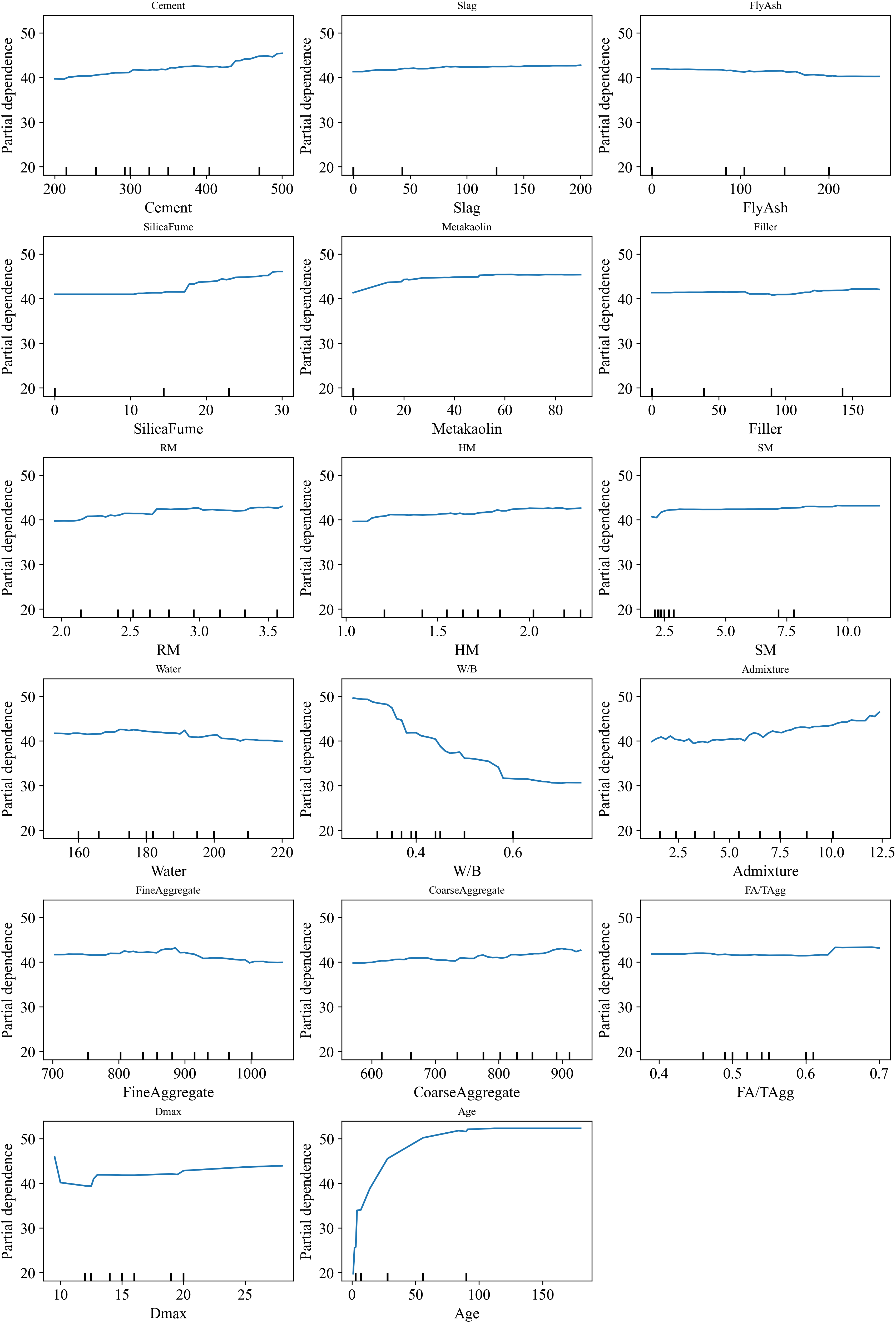
Figure 6: PDP for feature selection
After all consideration, the dataset is divided into training (80%) and test sets (20%). The K-fold cross-validation assesses the generalizability and performance of ML models across different subgroups of data samples. K-fold cross-validation is a commonly used method where the dataset is divided into K subsets [120,121]. In this approach, the model is trained on K-1 subsets, with the remaining subsets used for testing. This process is repeated K times, and the performance metrics are reported separately for each fold to evaluate the model’s performance across all subsets. In this study, 5-fold cross-validation was used: the training data was partitioned into five equal subsets, and in each iteration, the model was trained on four folds and validated on the remaining one. The final model, trained on the entire training set, was subsequently evaluated on the 20% test set, with the test results reported separately to demonstrate predictive performance on unseen data. For the CP method, the same preprocessing steps were applied, and LGBM and GBR were selected as the base models.
In this study, four ML algorithms including XGBoost, LGBM, GBR, and RF were selected based on their proven effectiveness for medium-sized tabular datasets. Tree-based ensemble methods serve as strong baselines for such data types due to their ability to model nonlinear relationships, capture feature interactions, and handle heterogeneous input features with minimal preprocessing. Recent comprehensive benchmarking studies by Grinsztajn et al. [122] and Borisov et al. [123] have demonstrated that gradient-boosted DTs consistently outperform deep neural networks on medium-sized tabular datasets, particularly under comparable hyperparameter tuning budgets. Moreover, these models exhibit lower computational costs and require fewer tuning parameters, which enhances their robustness and practical applicability. This trend is also evident in concrete-related applications. For instance, DT based models have shown superior performance over neural networks in predicting the compressive strength of alkali-activated concrete [124]. Furthermore, a previous study that evaluated 32 different ML algorithms identified XGBoost, GBR, AdaBoost, RF, and Bagging as the most suitable models for predicting concrete strength [6]. Based on this empirical evidence, the present study focuses on the top-performing and widely adopted tree-based models. The following section provides detailed description of the RF, GBR, LGBM, and XGboost algorithms.
RF is a widely used ensemble learning technique that builds multiple DTs during training and aggregates their outputs to improve predictive performance. In this method, each tree is trained on a random subset of the data, with random subsets of features considered for each split, introducing variability among the trees. This randomness reduces the risk of overfitting while maintaining the individual strength of the trees. Once the trees are generated, the final prediction is made by averaging the predictions (for regression tasks) or voting for the most common class (for classification tasks). RF is known for its robustness to noise and its ability to handle large datasets with high-dimensional features, providing accurate and reliable predictions even in complex tasks. Additionally, it offers built-in mechanisms for estimating variable importance and error, making it a powerful tool for both prediction and interpretation [125].
2.1.3 Gradient Boosting Regression
GBR is a boosting technique in ML that constructs a series of weak learners to form a highly accurate model. GBR add one weak learner at a time, with each learner trained to minimize the overall error of the model without modifying the previously added learners. Typically, regression trees are used as the weak learners, and a gradient-based optimization algorithm, such as stochastic gradient descent (SGD), is employed to iteratively train the model and minimize the loss. In the first iteration, the algorithm learns a weak learner (a tree) to reduce the training error. In subsequent iterations, each new tree is trained to correct the errors made by the previous trees. This process continues until the model achieves the desired level of performance, effectively reducing the overall error [126].
2.1.4 Extreme Gradient Boosting
XGBoost is a boosting ensemble model built on classification and regression trees (CART). It enhances the traditional GBR model by incorporating features, such as regularization, column subsampling, feature importance computation, and parallel processing. XGBoost forms its ensemble by iteratively training DTs, using gradient and second-order gradient information to improve the model’s predictive accuracy. In each iteration, the current gradients are calculated, and a new tree is fit to minimize the error. The model then updates its predictions, with regularization applied to control complexity and mitigate overfitting. The final prediction is obtained by weighting and summing the predictions of all the weak learners [3].
2.1.5 Light Gradient Boosting Machine
LGBM is a highly efficient ML model built on gradient boosting DTs. It stands out as a lightweight, high-performance framework, offering fast training and low memory usage, making it ideal for large-scale datasets. Unlike level-wise splitting algorithms (XGBoost), LGBM uses a leaf-wise splitting algorithm, where the leaf node with the highest gradient is split at each iteration. This method enables the model to quickly identify features and samples with the largest gradient, improving performance [3]. Table 3 summarizes the advantages and limitations of each model used in this study.

2.2 Hyperparameter Tuning and Model Evaluation
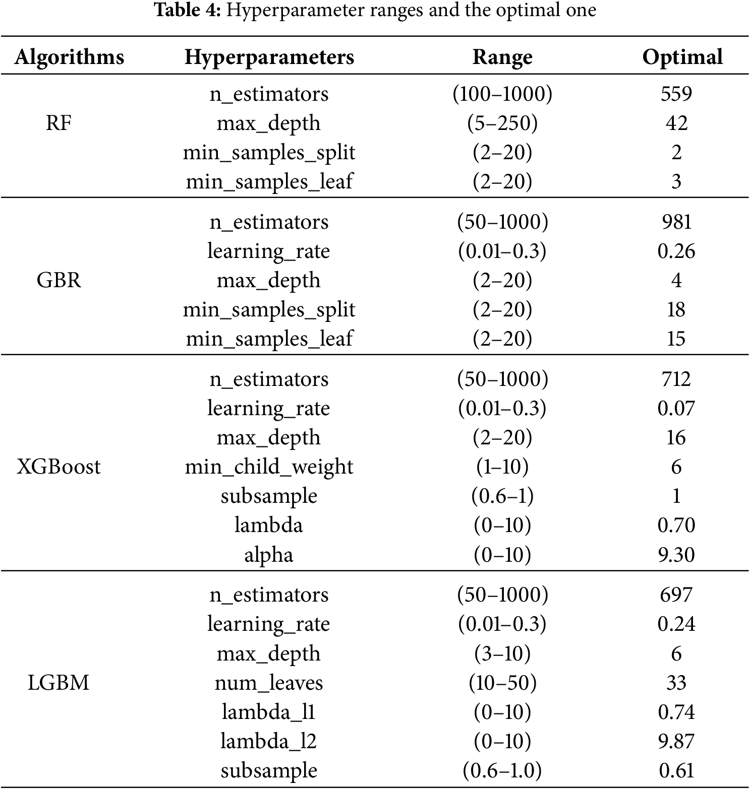
Hyperparameters are parameters that must be defined before the training process. While they influence the performance and behavior of a ML model, they are not learned from the data. The selection of hyperparameters can have a considerable effect on the model’s accuracy, generalization, and training duration. To achieve optimal performance, it is necessary to fine-tune these hyperparameters and experiment with various combinations by training several models. Afterward, the performance of these models is compared to determine the best configuration. As a result, optimizing hyperparameters is a crucial component of any ML algorithm [127]. To this end, for each ML model, random search is employed to optimize hyperparameters and identify the best-performing model. Compared to grid search and manual search, random search is more effective for hyperparameter optimization, even with the same number of combinations. This is because random search explores a broader hyperparameter space, increasing the likelihood of finding better-performing configurations [126]. The hyperparameters of each model and the optimal one is listed in Table 4.
Finally, to evaluate the predictive accuracy of all ML models in this study, the coefficient of determination (R2), root mean error (MSE), root mean square error (RMSE), mean absolute error (MAE), mean absolute relative error (MARE), and mean squared relative error (MSRE) are used.
2.3 SHapley Additive exPlanations
The output of ML models can be interpreted using SHAP, which constructs an additive interpretation model where each feature is considered a “contributor” to the prediction. For each sample, the model produces a predicted value, and SHAP assigns a value to each feature for that sample. If xi represents the i-th sample, and xij is the j-th feature of this sample, then the predicted value for the i-th sample is
where,
CP is a framework designed to generate prediction intervals that provide coverage guarantees, ensuring that the true target value lies within the predicted interval for a predefined proportion of new data points. The primary goal of CP is to construct prediction intervals that meet this coverage requirement without making strong assumptions about the data distribution. To achieve this, several methods have been developed within the CP framework, each offering different balances between computational and statistical efficiency [18,128].
Among the various approaches, split-CP is one of the simplest and most computationally efficient methods. It involves splitting dataset D into two disjoint subsets: the training set Dm = {(X1, Y1), …, (Xm, Ym)} and the calibration set Dn = {(Xm+1, Ym+1), …, (Xm+n, Ym+n)}. The training set is used to fit a predictive model
The prediction interval is then defined as:
While this method is interesting due to its simplicity and reduced computational cost, it can suffer from reduced statistical efficiency because part of the data is kept out for calibration. This limitation becomes particularly important when dealing with smaller datasets [18,128–130].
To overcome the statistical efficiency trade-off of split-CP, resampling methods, such as Jackknife+ and CV+ have been introduced. The Jackknife+ method is an enhancement of the traditional Jackknife approach, designed to provide predictive confidence intervals with theoretical coverage guarantees under minimal assumptions. It works by incorporating leave-one-out predictions for each training data point to account for variability in the model’s predictions. The process starts with fitting a regression model
For a new test point (Xn+1,Yn+1), the leave-one-out prediction
here,
To reduce computational time, the CV+ method can be used as an alternative to the leave-one-out approach. Similar to the Jackknife+ method, CV+ constructs prediction intervals through a cross-validation process, but with lower computational complexity. This method divides the training data into K disjoint subsets S1, S2, …, Sk, each of size m = n/K, where n is the total number of samples. For each fold k, a regression model
where k(i) identifies the fold containing sample i, ensuring that the model used to compute the residual does not have access to the data point itself during training. For a new test sample (Xn+1, Yn+1), the prediction interval is constructed as:
The CV+ method reduces computational costs compared to the Jackknife+ method, as it requires training only K models rather than n, making it more efficient for large datasets [17,131].
As explained, a common nonconformity measure is the absolute error between the predicted and actual values. This score results in constant interval width. In order to provide an adaptive CP method, the gamma conformity score is introduced, which is calculated as:
This approach is suitable for cases where the confidence interval is not symmetrical, and its range varies with the predicted values [129].
Another adaptive solution to the limitation of CV+ method is CQR which adapts the prediction intervals to the underlying distribution of the target variable, thereby addressing the issue of constant interval width inherent in absolute error-based nonconformity scores. The process begins with splitting the dataset into two parts: a training set and a calibration set. Using the training set, two quantile regression models are fitted to estimate the lower and upper quantiles of the target variable Y conditional on the features X, at specified levels αlo and αhi. These quantile models,
To ensure finite-sample validity, this interval is refined using the calibration set. For each sample in the calibration set, a conformity score is computed as:
Finally, for a new test point Xn+1, the prediction interval is adjusted based on the empirical distribution of the conformity scores from the calibration set. The final interval is:
where Q1−α(E) is the (1 − α)-th quantile of the conformity scores [132]. In this study, three conformal prediction methods, CV+, CV+_Gamma, and CQR, were implemented using MAPIE library to ensure efficient and reliable prediction interval estimation. For CV+ and CV+_Gamma, a 10-fold cross-validation strategy was employed to construct out-of-fold residuals. For CQR, 30% of the data was set aside as a calibration set. Prediction intervals were constructed for GBR and LGBM models at three significance levels: α = 0.10, 0.15, and 0.20, corresponding to 90%, 85%, and 80% confidence levels, respectively. The absolute error was used as the nonconformity score for CV+, while the gamma conformity score was used for CV+_Gamma. For CQR, prediction intervals were derived from the upper and lower quantiles and subsequently adjusted using conformity scores obtained from the calibration set.
Fig. 7 illustrates the results of 5-fold cross-validation in terms of R2, RMSE, and MAE for LGBM, XGboost, GBR and RF models. In contrast to the findings of previous studies on SCC where the results from 10-fold cross-validation demonstrated significant variation and instability across different folds [12,13,133], this study reveals highly stable performance. The R2, MAE, and RMSE metrics remain consistent across folds, underscoring the robustness and generalizability of our models. LGBM and XGBoost show relatively low RMSE and MAE values, indicating that they are effective in minimizing prediction errors. The similarity in performance between these two models highlights their strength and reliability, making them highly suitable for producing consistent and accurate predictions. The GBR model also shows great results, with slight variation in R2, indicating its robustness in predicting compressive strength of SCC. On the other hand, RF model shows the highest RMSE and MAE values among all the models, indicating a higher level of prediction error. Its R2 value, while consistent, is lower than those of the other models (0.85 in average). This higher level of error and lower consistency make RF a less optimal choice compared to other models; however, RF is still robust enough.
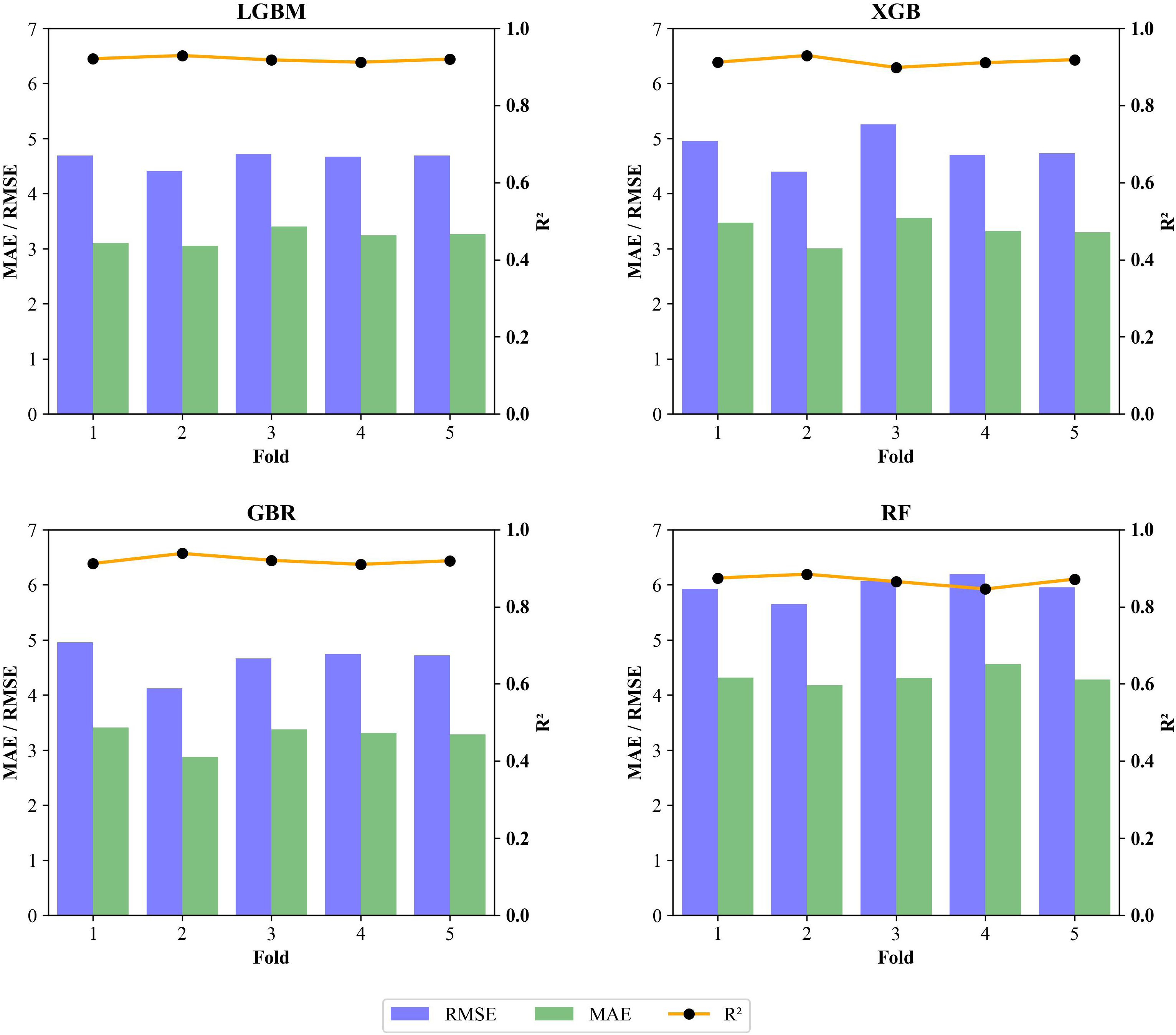
Figure 7: 5-fold cross-validation results of LGBM, XGBoost, GBR, and RF
The results shown in Fig. 8 provide a comparison of the predictive capabilities of LGBM, XGBoost, GBR, and RF models on the test set. LGBM demonstrates high degree of agreement between the predicted and actual strength values, with most points closely aligned along the diagonal, particularly within the ±20% tolerance band. The R2 of 0.95 and the mean R2 of 5-fold cross validation of 0.92 (Fig. 7) suggest that the model generalizes well to unseen data, maintaining strong predictive performance. The RMSE and MAE values are relatively low, indicating minimal prediction error. The XGBoost model displays almost the same performance as LGBM with an R2 of 0.95. The points are densely clustered around the diagonal line, and data align well within the tolerance bounds. The model achieves the low test RMSE and MAE, reflecting its strong ability to minimize error and produce accurate predictions. Both XGBoost and LGBM demonstrate the best overall performance, with high R2 values and low error metrics across the board, indicating excellent generalizability and predictive accuracy. GBR similarly shows strong performance with high R2. The RMSE and MAE (4.25 and 2.91, respectively) are comparable to XGBoost, confirming GBR’s high level of predictive accuracy. The RF model, however, exhibits higher prediction errors. The R2 of 0.90, although good, is lower than the other models. The RMSE and MAE values are also higher. The results confirm that all three boosting models, LGBM, XGBoost, and GBR, exhibit comparably high predictive accuracy, as indicated by their low RMSE and MAE reported in Table 5. Their strong performance can be attributed to the sequential learning mechanism inherent in boosting algorithms, where each successive learner focuses on correcting the residual errors of its predecessors. This iterative refinement allows the ensemble to capture complex, nonlinear relationships within the data, thereby enhancing prediction accuracy. These findings are further supported by the Taylor diagram (Fig. 9), which provide a visual summary of the standard deviation, correlation coefficient, and RMSE of each model relative to the observed data. As can be observed, the LGBM, XGBoost, and GBR models are tightly clustered near the reference line, indicating strong correlation with the actual values and a close match to the observed variability. Their proximity to the reference point and alignment along the lower centered RMSE reflect their superior accuracy and consistency. In contrast, the RF appears farther from the reference point, exhibiting a slightly higher standard deviation and lower correlation coefficient, indicating its relatively weaker predictive performance and greater deviation from the experimental values.
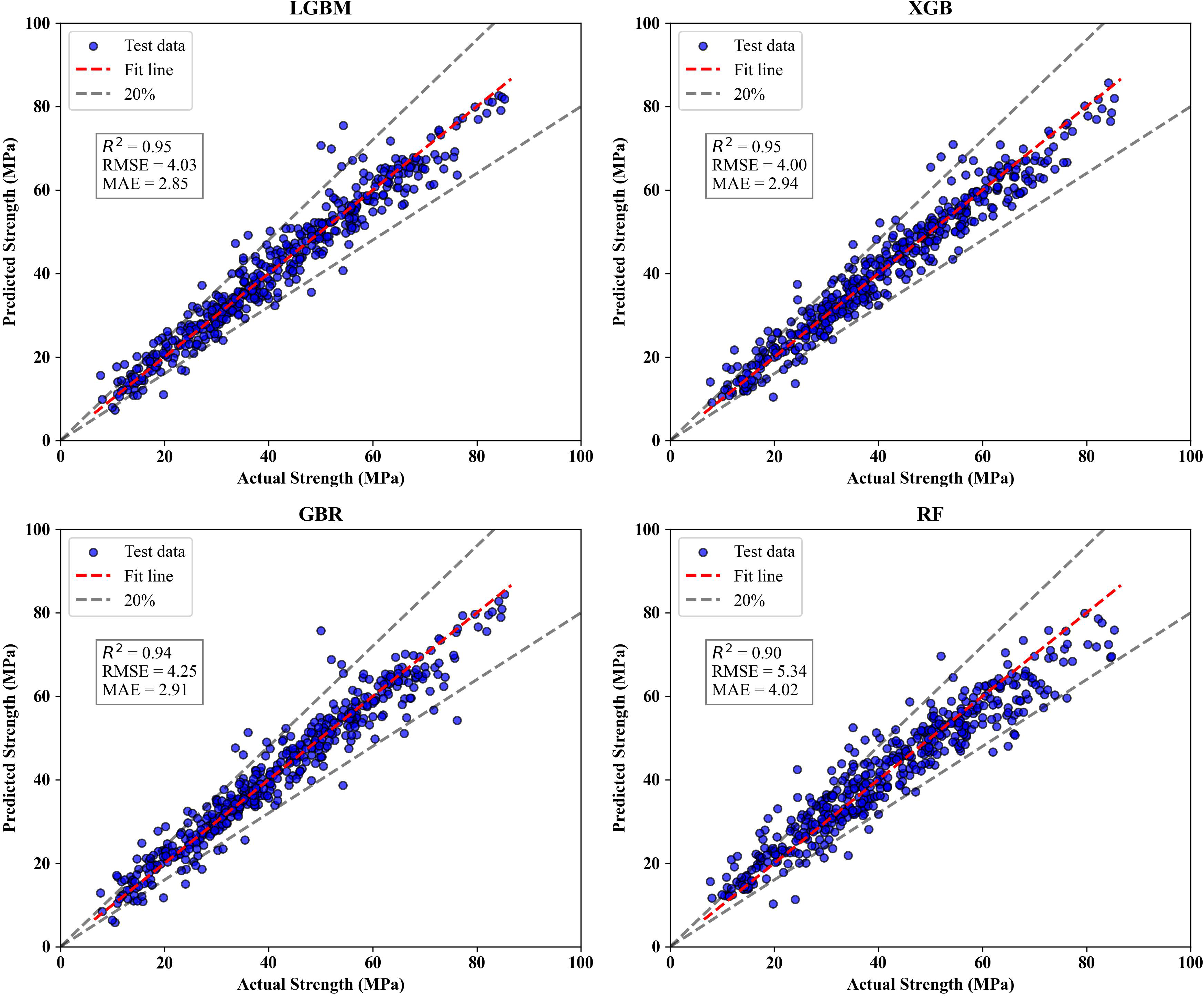
Figure 8: Predicted vs. actual compressive strength results with LGBM, XGBoost, GBR, and RF
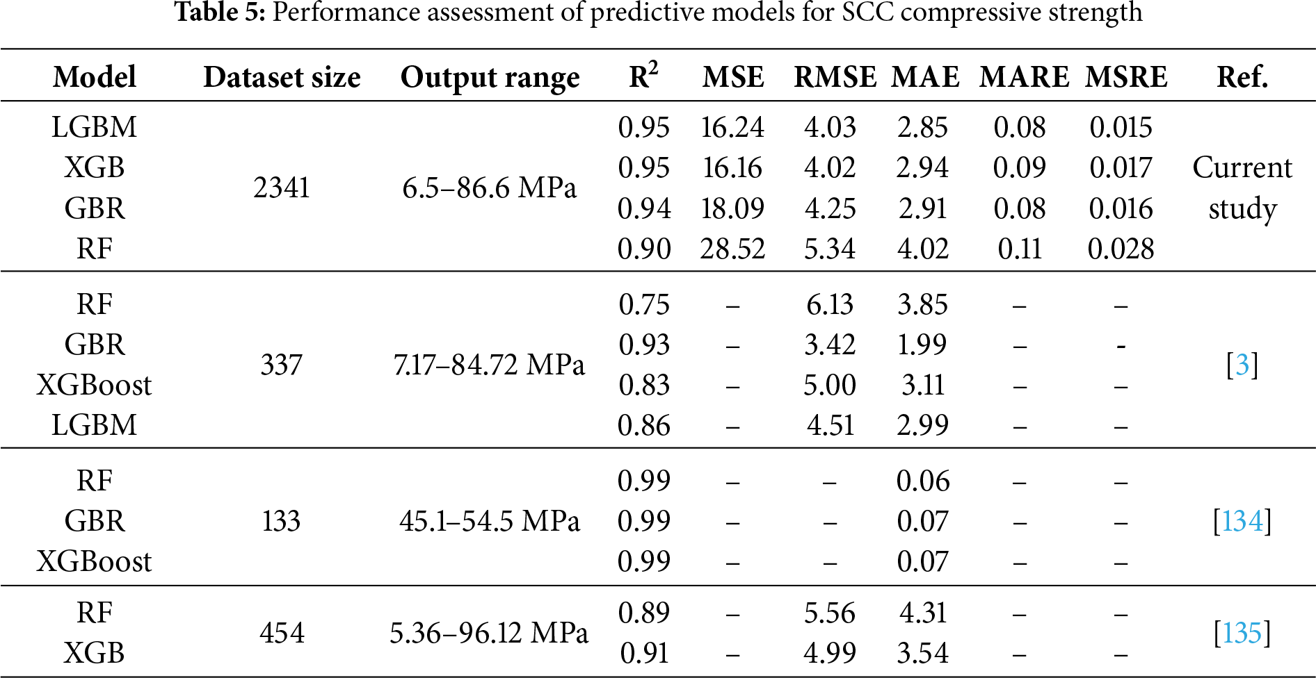
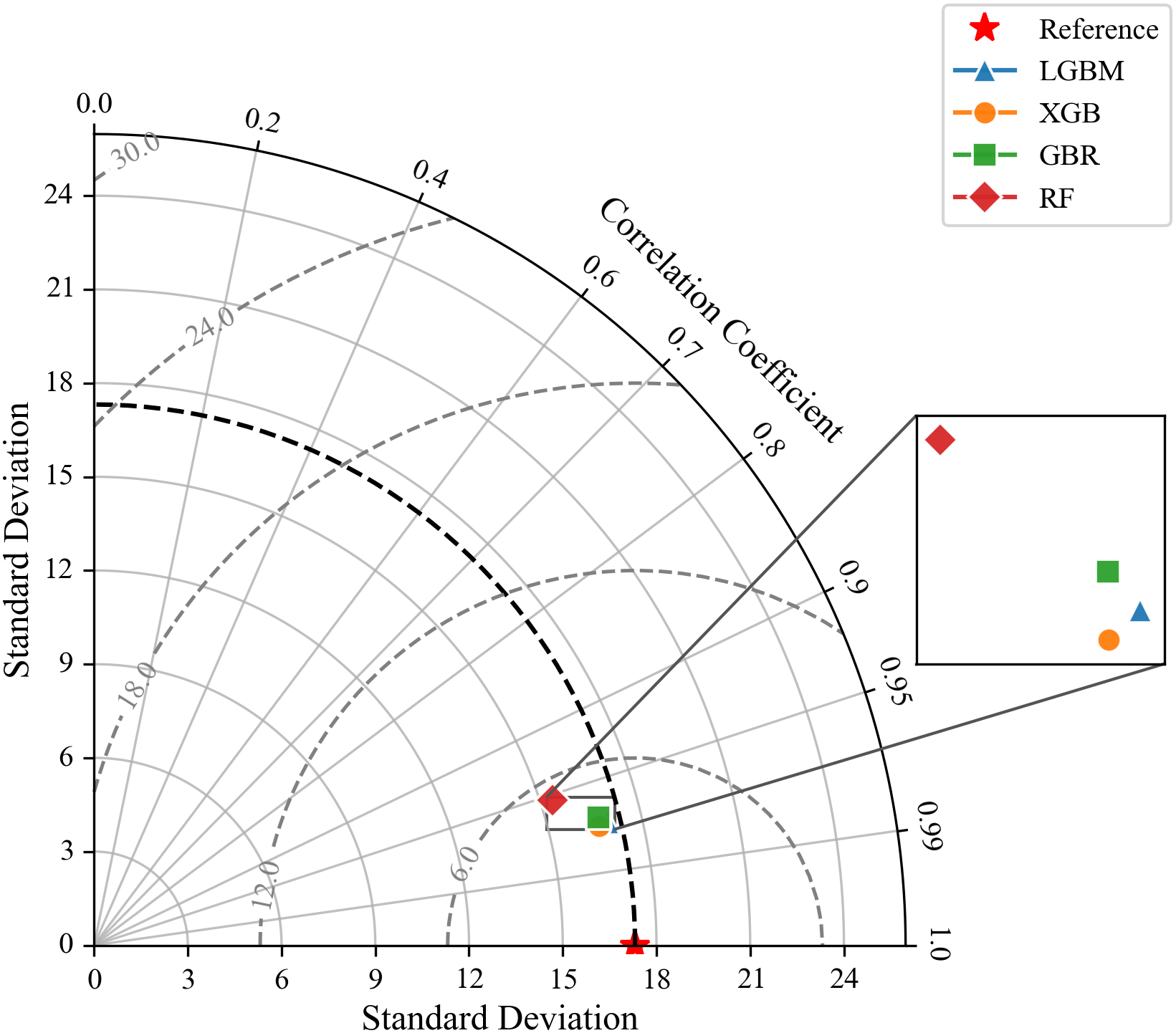
Figure 9: Taylor diagram of the applied ML models
A comparison between the results of the present study and previously published models for predicting SCC compressive strength is presented in Table 5. According to Ref. [3], the GBR model in that study outperformed its counterpart in this research; however, the other three models evaluated here, LGBM, XGBoost, and RF, exhibited superior performance. This observation aligns with the No Free Lunch Theorem (NFL), which states that no single model consistently outperforms others across all problems. Model performance is often dataset-dependent, and the most suitable model may vary depending on the specific characteristics of the data. In the case of Ref. [134], the reported performance metrics appear better than those obtained in the current study. However, this difference should be interpreted cautiously, as dataset size and output range are critical factors influencing error metrics. Their dataset contains only 133 samples with a narrow compressive strength range (45.1–54.5 MPa), which inherently reduces variability and simplifies the prediction task. In contrast, the current study uses a much larger dataset (2341 samples) with a broader strength range (6.5–86.6 MPa) collected from multiple sources. The increased variability and potential noise from different experimental conditions make the prediction task more challenging, yet more representative of real-world scenarios. Regarding Ref. [135], which is closer to the present study in terms of dataset size (454 samples) and strength range, our models demonstrate improved predictive accuracy, particularly in terms of RMSE and MAE.
Fig. 10 shows the performance of LGBM, XGBoost, GBR, and RF models through residual plots and error distribution box plots. The residual plots, shown at the top, provide insights into how the predicted values align with the actual values across the range of compressive strength for each model in the test set.
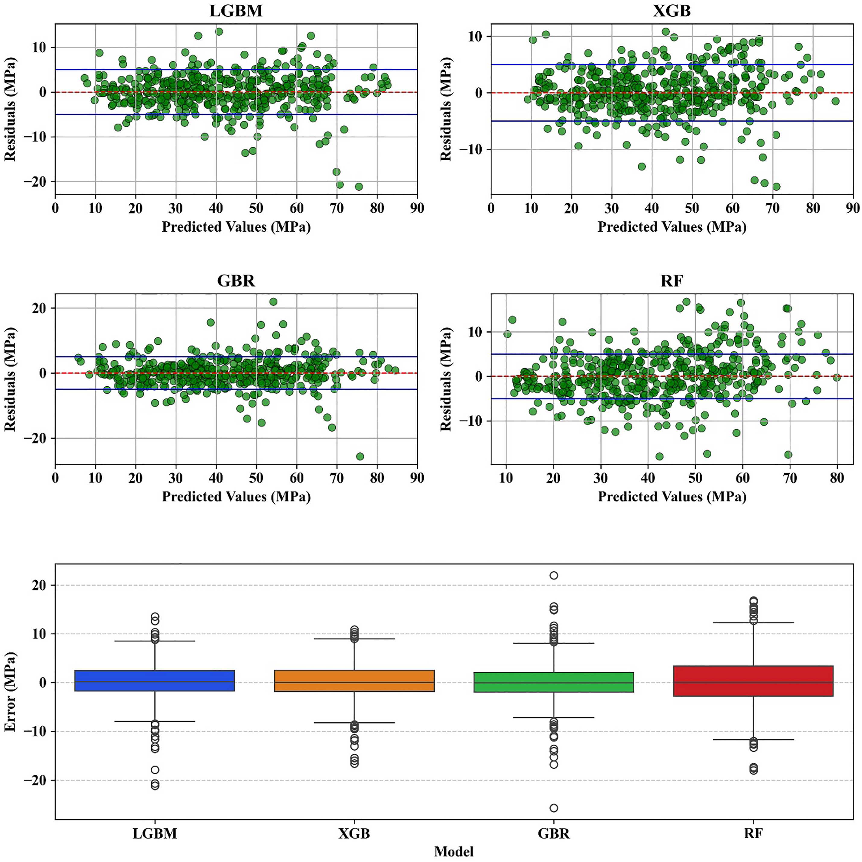
Figure 10: Residual analysis with LGBM, XGBoost, GBR, and RF
For all four models, the residuals appear relatively symmetrically distributed around zero, though some variance is observed. This suggests that the models capture the general trends in the data reasonably well, but slight deviations are present. Both LGBM and XGBoost exhibit residuals that remain largely clustered within ±5 MPa, indicating that their predictions closely track the actual values. This tight clustering around zero for both models suggests that they consistently produce accurate estimates, with only a small fraction of predictions deviating significantly. In contrast, the RF model displays a much wider dispersion, with residuals frequently within ±10 MPa. This indicates that RF predictions are more variable and less reliable in terms of precision.
Each model’s box plot provides a comparison of how well it performs in terms of variability and central tendency. None of the models exhibit a consistent bias towards over- or under-prediction, as seen by the median error for all models being near zero. However, there are clear differences in the error spread and the presence of outliers. LGBM, GBR, and XGBoost show narrower interquartile range (IQR), demonstrating the higher consistency and reliability compared to RF. The RF model, with the widest IQR and the most outliers, indicates the highest level of error variability, highlighting that it is the least consistent of the four models.
The SHAP summary plot (Fig. 11) presents the impact of individual input features on the model’s output, providing insights into both their relative importance and their direction of influence on the predicted compressive strength of SCC. Each plot ranks the features according to their contribution to the model predictions, where blue and red colors represent low and high feature values, respectively. Across all four models, age, W/B, cement content and admixture dosage consistently emerge as the most influential parameters on SCC compressive strength. However, variations in the ranking of the remaining features reflect differences in each algorithm’s tree construction strategy, split selection criterion, and regularization scheme. For example, LGBM uses a leaf-wise growth strategy, expanding the leaf with the highest split gain, regardless of its depth, whereas XGB uses a level-wise growth strategy, expanding all nodes at a given depth before proceeding to the next level.
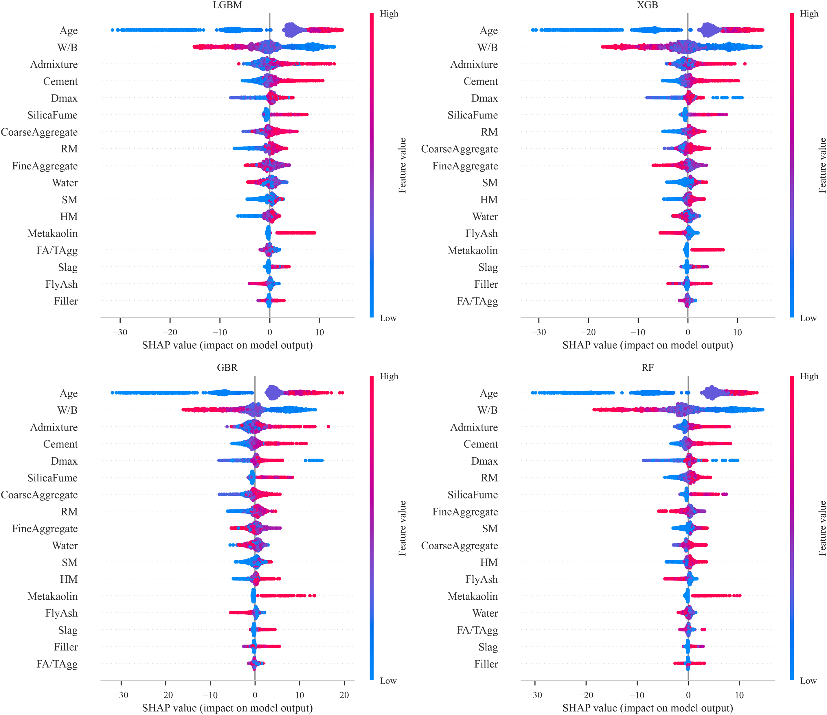
Figure 11: SHAP summary plot of LGBM, XGB, GBR, and RF models
As it is clear, higher age values are associated with positive SHAP values, indicating that compressive strength increases with curing time due to prolonged hydration of cement and SCMs, leading to enhanced microstructural development [3]. Similarly, greater cement content exhibits a positive contribution, confirming its direct effect on strength gain. In contrast, higher W/B ratios negatively impact compressive strength, consistent with well-established findings in SCC research [136]. The results also reveal that RM and SM have noticeable impact on SCC strength, whereas SCMs show a comparatively smaller impact on model predictions. However, this lower apparent influence may be attributed to the limited number of data point containing SCMs in the dataset, as reflected in the statistical distribution presented in Table 2, where most entries are zero. Hence it cannot be concluded that SCMs have no significant influence on compressive strength.
3.5 Conformal Prediction Results
3.5.1 Actual vs. Predicted Strength with Prediction Intervals
Figs. 12 and 13 demonstrate the prediction intervals produced by the CV+, CV+_Gamma, and CQR methods for the LGBM and GBR models at target coverage levels of 90%, 85%, and 80%. These target coverage levels reflect how effectively each method captures the true compressive strength values while also revealing differences in their prediction accuracy and adaptability across the models. In Fig. 12, for the 90% target coverage, the CV+ method achieved a coverage of 93%, slightly surpassing the target. This method produced relatively narrow prediction intervals, with an average width of 16.84. The narrower intervals indicate that CV+ effectively balances accuracy and precision, offering tight ranges that still include most of the true values. However, its intervals remained relatively consistent across the prediction range, limiting the method’s ability to adapt to varying levels of uncertainty in the predictions.
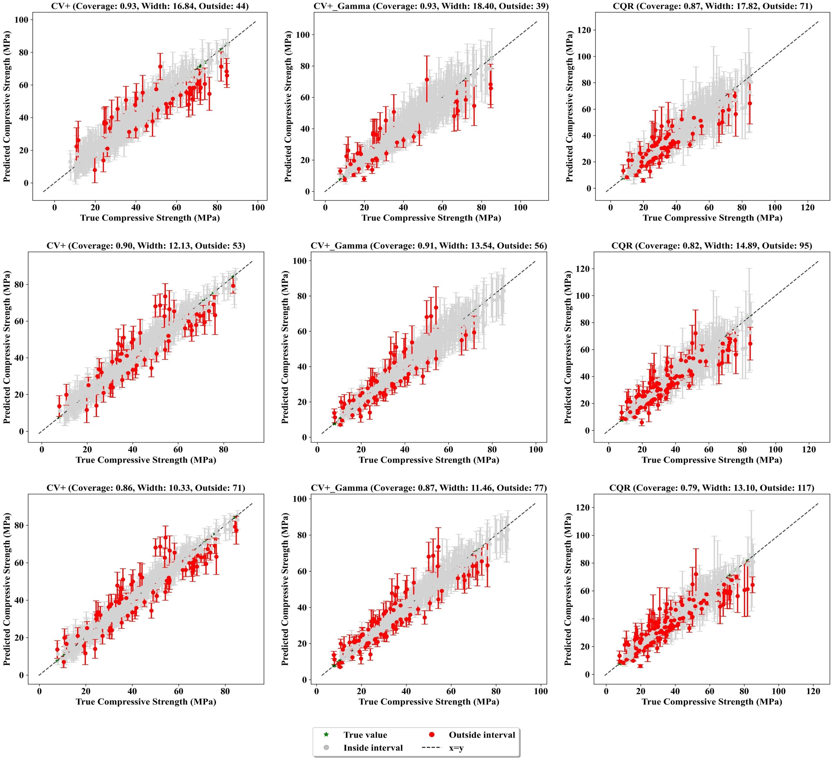
Figure 12: Actual values vs. prediction intervals of compressive strength at different coverage levels (LGBM)
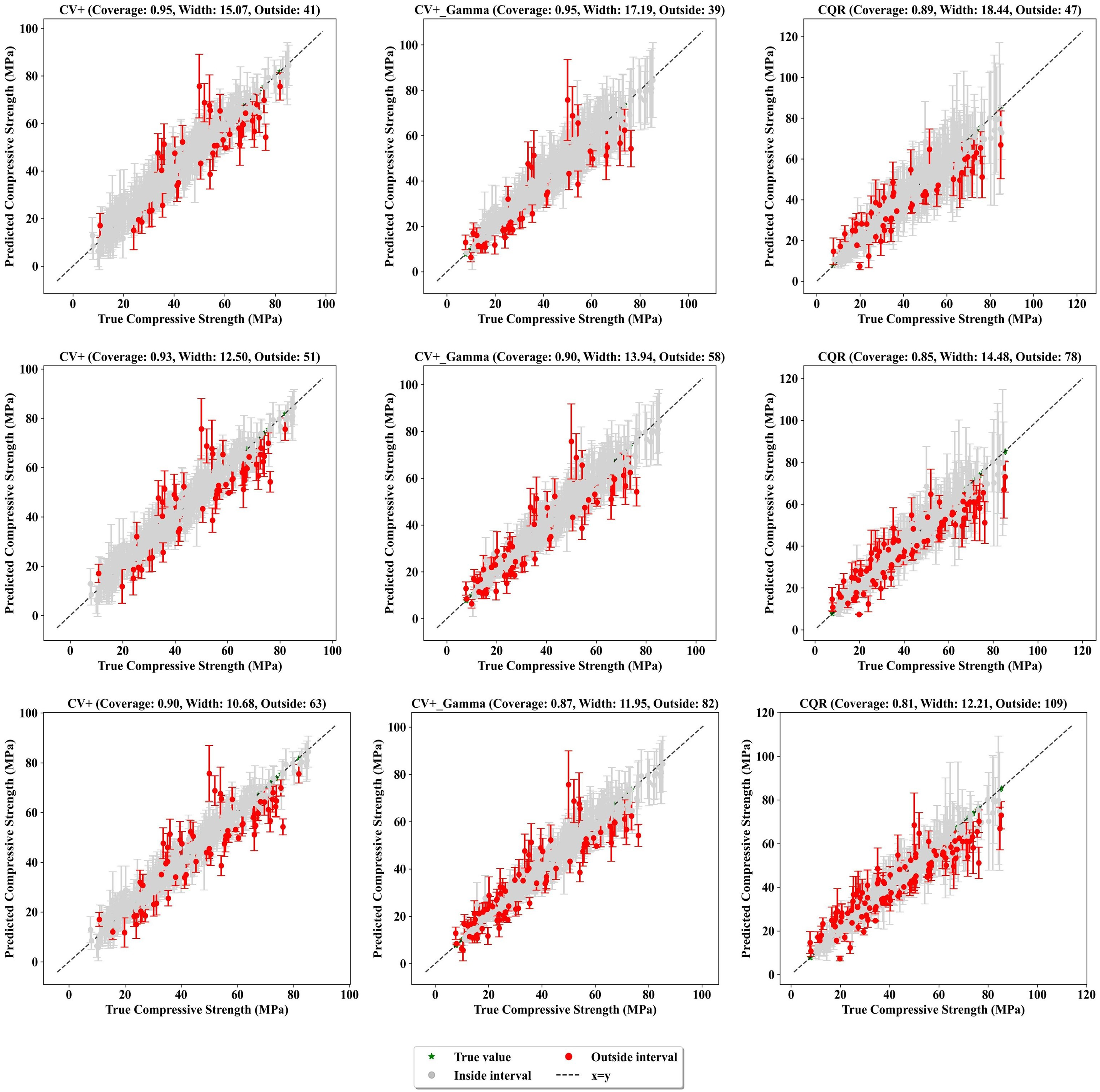
Figure 13: Actual values vs. prediction intervals of compressive strength at different coverage levels (GBR)
The CV+_Gamma method, on the other hand, incorporates a Gamma conformity score to adjust the interval size based on the magnitude of the predictions. It achieved a coverage of 93%, with an average interval width of 18.40. Unlike CV+, the CV+_Gamma intervals adapt to the predicted values, becoming wider when the predicted strength increases. The CQR method achieved a coverage of 87%, lower than the targeted coverage and showed the highest interval with an average of 17.82. CQR is specifically designed to handle heteroscedasticity, where variability in the data changes across the target range. This adaptability is reflected in the interval widths, which expand at both lower and higher predicted strengths where uncertainty is more pronounced. A shown in Fig. 13, the GBR model produced results comparable to those of the LGBM model, though it occasionally resulted in slightly wider intervals and higher coverage.
A clear trend emerges when comparing different target coverage levels. As the target coverage decreases from 90% to 85% and then 80%, the prediction intervals become narrower. While this can improve precision, it comes at the cost of more points being outside prediction intervals. For instance, considering the CV+_Gamma approach with the LGBM model (Fig. 12), the number of points falling outside the prediction intervals increases from 39 at 90% coverage to 56 at 85% and 77 at 80% coverage. This demonstrates the trade-off between interval size and reliability; narrower intervals mean greater precision but a higher risk of missing the true values.
Based on the graphs, it can be concluded that higher coverage levels ensure most true compressive strengths are captured, providing a conservative and reliable approach. However, the trade-off is wider intervals, which may limit their practical usefulness in applications requiring precise estimates, such as material optimization or cost reduction. Conversely, lower coverage levels produce tighter intervals but increase the likelihood of underestimating or overestimating the true compressive strength.
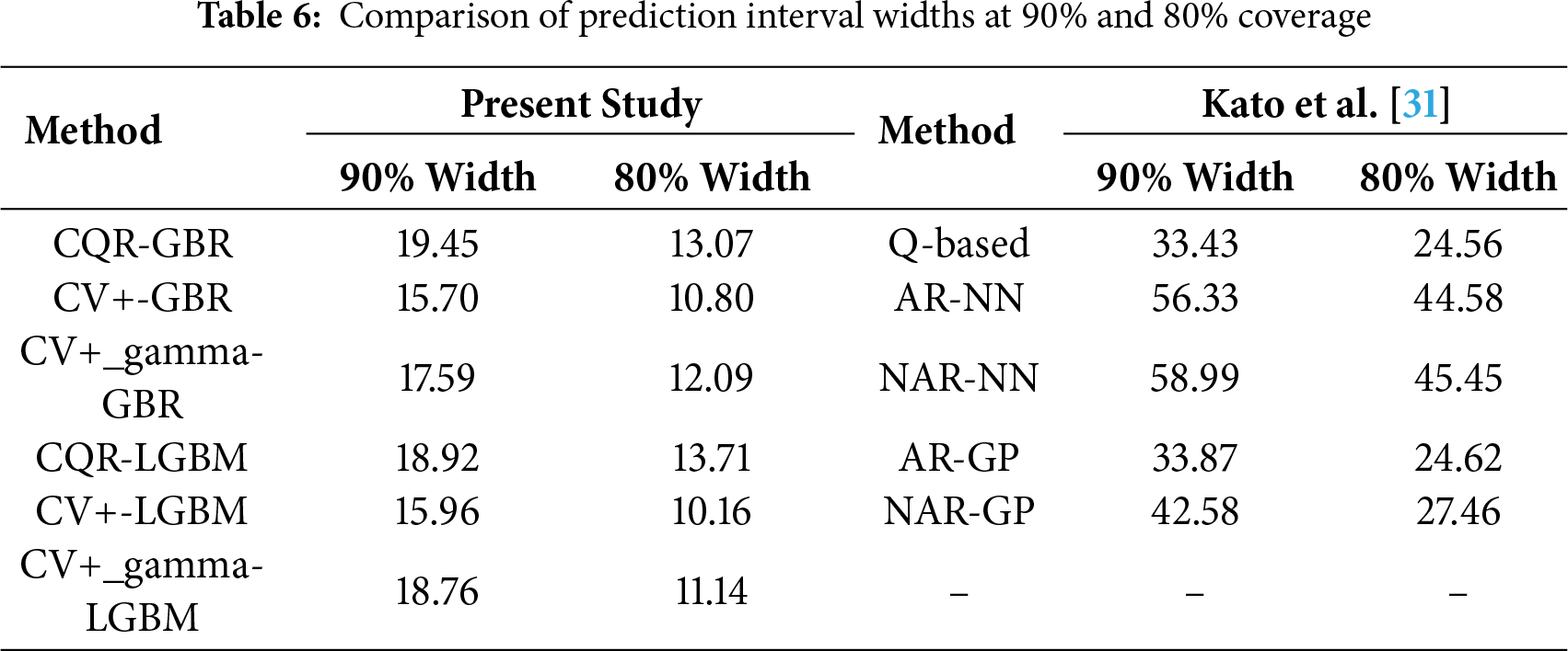
Kato et al. [31] applied CP to concrete dataset available in UCI repository. They compared the performance of three different nonconformity scores, including (i) absolute residual (AR), (ii) normalized absolute residual (NAR), and (iii) quantile-based (Q-based) methods. The base models employed in their study were quantile regression, neural networks (NN), and Gaussian processes (GP). The average prediction interval widths corresponding to 90% and 80% coverage levels for various nonconformity scores and models are presented in Table 6. In comparison, the fine-tuned ensemble models used in our study achieved narrower interval widths with the same nonconformity scores, demonstrating superior performance.
3.5.2 Conditional Coverage and Interval Width Results
Figs. 14 and 15 illustrate the conditional coverage and the prediction interval widths across different compressive strength ranges for both LGBM (top) and GBR (bottom). In Fig. 14, the dashed horizontal line indicates the target coverage level of 90%. Conditional Coverage is an important characteristic of prediction intervals, ensuring their reliability and adaptability across diverse input conditions. It means that the intervals can flexibly adjust their size based on the complexity or difficulty of the input data while aiming to maintain the desired coverage level of 1 − α. Although the coverage may sometimes exceed 1 − α for certain values and fall below it for others, the overall objective is to achieve consistent prediction intervals with 1 − α coverage across all training and test data. This ensures that the intervals are informative and capable of providing robust uncertainty quantification for a wide range of inputs [17]. To report the conditional coverage, the test set is divided into 10 bins based on the quantiles of the actual values of the output.

Figure 14: Conditional coverage of CV+, CV+_Gamma, and CQR methods at target coverage of 90%
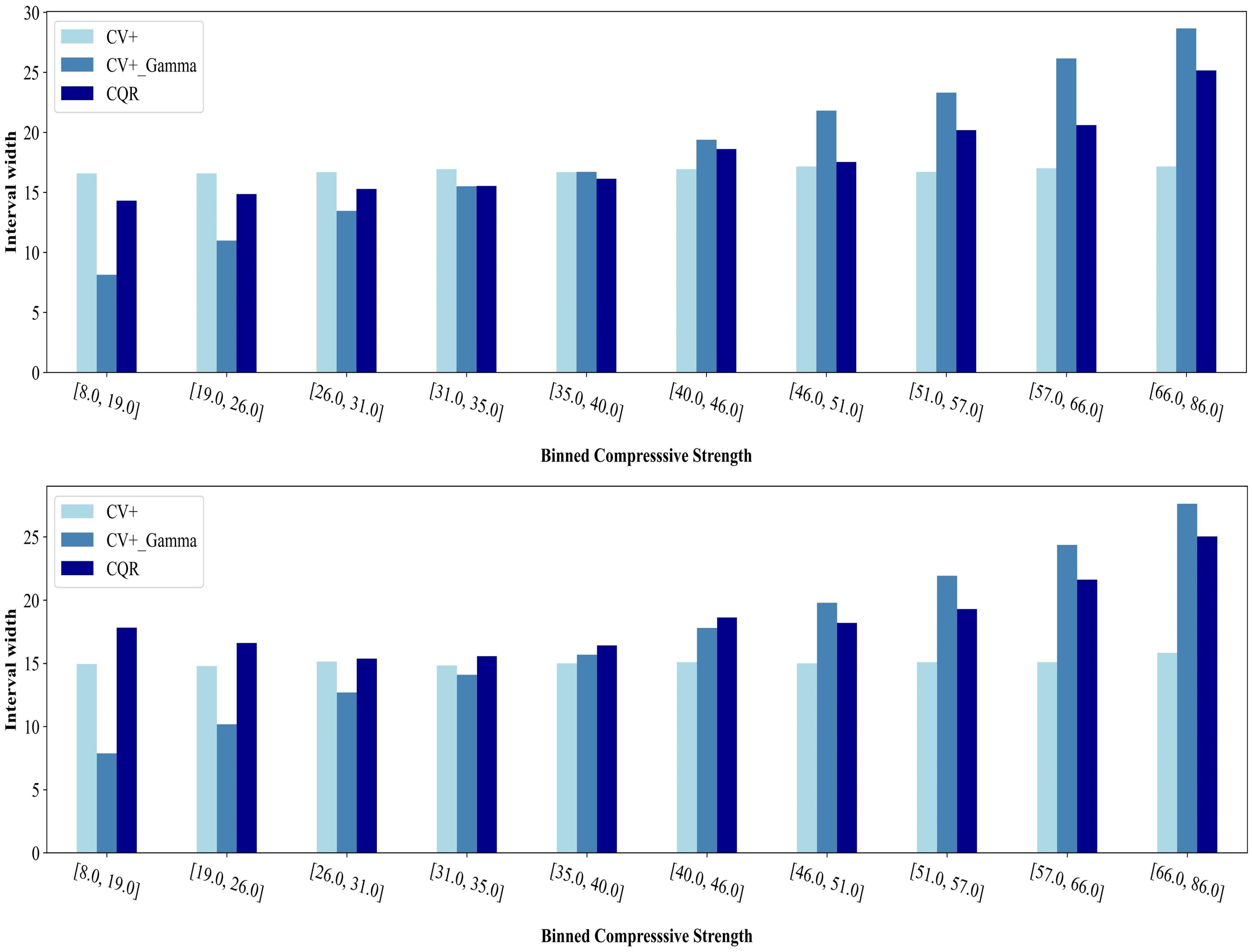
Figure 15: Prediction intervals at binned compressive strength
For the LGBM model (Fig. 9), the CV+ method demonstrates generally consistent performance across most bins, especially in the low and mid-range compressive strength categories. However, for the highest strength bin (66.0–86.0 MPa), the conditional coverage falls below the target level. Notably, for all strength bins, the CV+ method produces intervals of the same width (Fig. 15). The CV+_Gamma method underperforms in the lowest strength bin (8.0–19.0 MPa), with coverage below the target, but it achieves the narrowest intervals in this range, showcasing the trade-off between validity and efficiency [17]. Compared to LGBM model, the GBR provides better conditional coverage for CV+_Gamma as it meets the coverage in most bins.
As compressive strength increases, its intervals widen to reflect the growing uncertainty in higher-strength predictions. The CQR approach maintains stable and reliable performance in the mid-strength bins for LGBM, but at the highest strengths, coverage falls below the target. While CQR typically yields the widest intervals in the low- and mid-strength bins, it begins to outperform CV+_Gamma in higher-strength scenarios by providing more reliable sized intervals; however, it compromises the coverage level.
The performance patterns of CV+, CV+_Gamma, and CQR in GBR model are similar to those observed with LGBM, though the coverage and interval widths vary in magnitude due to the calibration specific to each model. Similar to LGBM, CV+ maintains relatively stable coverage in the lower bins, while CQR and CV+_Gamma display varying degrees of the validity-efficiency trade-off.
Considering the trade-offs observed across different compressive strength ranges, the CV+_Gamma method offers a more balanced compromise between coverage and interval width. While it may fail to achieve the target coverage in the lowest strength bin, it simultaneously provides the narrowest intervals where such efficiency might be most valuable. As compressive strength increases and the underlying complexity grows, CV+_Gamma broadens its intervals. This adaptive approach accounts for greater uncertainty and ensures more robust predictive coverage under more challenging conditions.
The results of this study showed that all four ML models produced consistent and stable predictions across the five cross-validation folds, demonstrating strong generalizability and robustness. In contrast, some studies have reported substantial fluctuations in model performance across folds. For example, using 10-fold cross-validation, models based on bagging regressors showed wide variability in results, with R2 ranging from 0.1 to 1.0, MAE from 5 to 20 MPa, and RMSE from 7 to 19 MPa [133]. Similarly, Phan and Nguyen [12]. Reported that the Adaboost model yielded R2 values between 0.70 and 0.97, MAE between 1.09 and 6.29 MPa, and RMSE between 1.48 and 11.04 MPa. Such large variations in R2, MAE, and RMSE indicate that the performance of these models was highly sensitive to the specific data subsets used during training and validation. This level of inconsistency is often a sign of overfitting, where the model memorizes patterns specific to certain folds rather than learning a generalizable relationship within the dataset [32]. Several factors may contribute to this instability, including small or imbalanced datasets that make the model more susceptible to the effects of partitioning, insufficient or poorly selected input features that fail to capture the true complexity of the problem, and the absence of proper regularization techniques. Moreover, the use of overly complex models without adequate tuning can further worsen this issue by fitting noise in the training data. In contrast, the models developed in this study, particularly the ensemble boosting models (LGBM, XGBoost, and GBR) demonstrated superior and stable performance due to several factors. First, the sequential nature of boosting allows each learner to correct the errors of its predecessor, enabling the ensemble to effectively capture complex, nonlinear relationships in the data. Additionally, the comprehensive feature set, which includes both material composition and chemical descriptors such as reactivity moduli, allowed the models to account for the combined physical and chemical influences on concrete strength, improving prediction accuracy and reducing overfitting. Finally, the robustness of these models was further enhanced by the regularization techniques inherent in boosting algorithms and careful hyperparameter tuning.
In addition to providing stable point predictions, the conformal prediction results further demonstrate the robustness of the developed models. By providing calibrated prediction intervals that closely align with target coverage levels, CP improves model reliability beyond what traditional approaches offer. For example, the CV+_Gamma method consistently achieved empirical coverage near the desired 90% threshold while maintaining relatively narrow intervals. This indicates that the models not only produced accurate predictions but also reliably quantified the uncertainty associated with them.
The practical utility of CP becomes particularly evident in mix design optimization. While a point prediction (e.g., 50 MPa) represents the model’s best estimate, the corresponding prediction interval (e.g., 45–55 MPa at 90% coverage) reflects the range within which the realized strength is likely to fall under typical field variability. Such variability may result from differences in raw material properties, including cement chemistry, aggregate grading, or SCM fineness, as well as curing conditions such as temperature, humidity, and duration. Consequently, prediction intervals enable engineers to evaluate not only the expected performance of a mix but also its robustness. A narrow interval suggests that the mix is less sensitive to variations in materials and curing, whereas a wider interval highlights greater sensitivity and potential risk.
This study investigated the application of ML models and CP to predict the compressive strength of SCC, while incorporating uncertainty quantification. Using a comprehensive dataset of 3005 samples and applying ensemble learning algorithms, including RF, GBR, XGBoost, and LGBM, the study demonstrated the capability of these models to accurately predict SCC compressive strength and assess the reliability of their prediction. The main findings can be summarized as follows:
• Boosting-based models (LGBM, XGB, and GBR) demonstrated the highest predictive accuracy, with R2 values exceeding 0.94 on the test data. The residuals were tightly distributed around zero, reflecting strong generalization and minimal prediction bias.
• The integration of well-structured feature sets, including material and chemical descriptors (e.g., reactivity moduli), combined with careful model tuning significantly enhanced model robustness and predictive stability.
• SHAP analysis identified curing age, W/B, cement content, and admixture dosage as the most influential parameters affecting SCC compressive strength.
• As expected, reducing the target coverage from 90% to 85% and 80% resulted in narrower prediction intervals, improving precision at the expense of coverage. For example, for the LGBM model using the CV+_Gamma method, the number of points outside coverage increased from 39 to 77 as the confidence level decreased.
• The CV+_Gamma method emerged as the most balanced approach, effectively adjusting interval widths based on compressive strength levels to handle increasing uncertainty. While it underperformed at low-strength ranges, it provided reliable coverage and efficiency at higher strengths.
While the proposed framework effectively predicts compressive strength and quantifies uncertainty via CP, it currently focuses on a single property and omits fresh and rheological characteristics, such as workability (e.g., slump flow) and setting time that are critical for practical SCC mixture design. Future work should integrate these properties into a unified ML pipeline (e.g., multi-task regression) to better reflect real-world requirements. In parallel, exploring additional learning algorithms and advancing conformal prediction, especially through problem-specific, adaptive nonconformity scores that produce efficient, data-dependent intervals would improve reliability of the uncertainty estimates and broaden applicability across diverse concrete compositions and performance targets.
Acknowledgement: The authors wish to thank the financial support of the National Science and Engineering Research Council of Canada (NSERC) and the ten industrial partners participating in the NSERC Industrial Research Chair (IRC) on Development of Flowable Concrete with Adapted Rheology and Their Application in Concrete Infrastructures, held by Professor Ammar Yahia at the Université de Sherbrooke.
Funding Statement: This research was conducted as part of the activities of the NSERC Industrial Research Chair (IRC) on Development of Flowable Concrete with Adapted Rheology and Their Application in Concrete Infrastructures, held by Professor Ammar Yahia at the Université de Sherbrooke. The Chair is financially supported by the Natural Sciences and Engineering Research Council of Canada (NSERC; Grant No. ALLRP 576708-22) and ten industrial partners. No specific funding was received for this particular study.
Author Contributions: The authors confirm contribution to the paper as follows: Conceptualization, Fatemeh Mobasheri, Masoud Hosseinpoor, Ammar Yahia and Farhad Pourkamali-Anaraki; methodology, Fatemeh Mobasheri, Masoud Hosseinpoor, Ammar Yahia and Farhad Pourkamali-Anaraki; validation, Fatemeh Mobasheri, Masoud Hosseinpoor, Ammar Yahia and Farhad Pourkamali-Anaraki; writing-review and editing, Fatemeh Mobasheri, Masoud Hosseinpoor, Ammar Yahia and Farhad Pourkamali-Anaraki; formal analysis, Fatemeh Mobasheri, Masoud Hosseinpoor, Ammar Yahia and Farhad Pourkamali-Anaraki; investigation, Fatemeh Mobasheri, Masoud Hosseinpoor, Ammar Yahia and Farhad Pourkamali-Anaraki; data curation, Fatemeh Mobasheri, Masoud Hosseinpoor, Ammar Yahia and Farhad Pourkamali-Anaraki; writing—original draft preparation, Fatemeh Mobasheri, Masoud Hosseinpoor, Ammar Yahia and Farhad Pourkamali-Anaraki; visualization, Fatemeh Mobasheri; supervision, Ammar Yahia, Masoud Hosseinpoor and Farhad Pourkamali-Anaraki; project administration, Ammar Yahia and Farhad Pourkamali-Anaraki;funding acquisition, Ammar Yahia. All authors reviewed the results and approved the final version of the manuscript.
Availability of Data and Materials: The data used in this study were compiled from previously published sources, including 64 journal articles, 2 conference papers, and 16 theses conducted at the Université de Sherbrooke, as cited in references [34–115]. The compiled dataset was further curated and processed as part of an ongoing research project at the Université de Sherbrooke. While the raw data from the cited publications are publicly available through their respective sources, the processed dataset used for model development is not publicly available at this time due to ongoing research.
Ethics Approval: Not applicable.
Conflicts of Interest: The authors declare no conflicts of interest to report regarding the present study.
References
1. Naik TR, Kumar R, Ramme BW, Canpolat F. Development of high-strength, economical self-consolidating concrete. Constr Build Mater. 2012;30(7):463–9. doi:10.1016/j.conbuildmat.2011.12.025. [Google Scholar] [CrossRef]
2. Akram T, Memon SA, Obaid H. Production of low cost self compacting concrete using bagasse ash. Constr Build Mater. 2009;23(2):703–12. doi:10.1016/j.conbuildmat.2008.02.012. [Google Scholar] [CrossRef]
3. Huang P, Dai K, Yu X. Machine learning approach for investigating compressive strength of self-compacting concrete containing supplementary cementitious materials and recycled aggregate. J Build Eng. 2023;79(10):107904. doi:10.1016/j.jobe.2023.107904. [Google Scholar] [CrossRef]
4. Aggarwal S, Singh R, Rathore A, Kapoor K, Patel M. A novel data-driven machine learning techniques to predict compressive strength of fly ash and recycled coarse aggregates based self-compacting concrete. Mater Today Commun. 2024;39:109294. doi:10.1016/j.mtcomm.2024.109294. [Google Scholar] [CrossRef]
5. Shafighfard T, Bagherzadeh F, Rizi RA, Yoo D-Y. Data-driven compressive strength prediction of steel fiber reinforced concrete (SFRC) subjected to elevated temperatures using stacked machine learning algorithms. J Mater Res Technol. 2022;21(3):3777–94. doi:10.1016/j.jmrt.2022.10.153. [Google Scholar] [CrossRef]
6. Kazemi F, Shafighfard T, Jankowski R, Yoo D-Y. Active learning on stacked machine learning techniques for predicting compressive strength of alkali-activated ultra-high-performance concrete. Arch Civ Mech Eng. 2025;25(1):24. doi:10.1007/s43452-024-01067-5. [Google Scholar] [CrossRef]
7. Golafshani E, Khodadadi N, Ngo T, Nanni A, Behnood A. Modelling the compressive strength of geopolymer recycled aggregate concrete using ensemble machine learning. Adv Eng Softw. 2024;191:103611. doi:10.1016/j.advengsoft.2024.103611. [Google Scholar] [CrossRef]
8. Özyüksel Çiftçioğlu A, Kazemi F, Shafighfard T. Grey wolf optimizer integrated within boosting algorithm: application in mechanical properties prediction of ultra high-performance concrete including carbon nanotubes. Appl Mater Today. 2025;42(289):102601. doi:10.1016/j.apmt.2025.102601. [Google Scholar] [CrossRef]
9. Farooq F, Czarnecki S, Niewiadomski P, Aslam F, Alabduljabbar H, Ostrowski KA, et al. A comparative study for the prediction of the compressive strength of self-compacting concrete modified with fly ash. Materials. 2021;14(17):4934. doi:10.3390/ma14174934. [Google Scholar] [PubMed] [CrossRef]
10. Kumar S, Kumar R, Rai B, Samui P. Prediction of compressive strength of high-volume fly ash self-compacting concrete with silica fume using machine learning techniques. Constr Build Mater. 2024;438(4):136933. doi:10.1016/j.conbuildmat.2024.136933. [Google Scholar] [CrossRef]
11. Rajakarunakaran SA, Lourdu AR, Muthusamy S, Panchal H, Alrubaie AJ, Jaber MM, et al. Prediction of strength and analysis in self-compacting concrete using machine learning based regression techniques. Adv Eng Softw. 2022;173(1):103267. doi:10.1016/j.advengsoft.2022.103267. [Google Scholar] [CrossRef]
12. Phan T-D, Nguyen D-L. Data-driven approaches for predicting and optimizing the compressive strength of self-compacting concrete. Mater Today Commun. 2025;42(3):111298. doi:10.1016/j.mtcomm.2024.111298. [Google Scholar] [CrossRef]
13. Wang Z, Liu H, Amin MN, Khan K, Qadir MT, Khan SA. Optimizing machine learning techniques and SHapley Additive exPlanations (SHAP) analysis for the compressive property of self-compacting concrete. Mater Today Commun. 2024;39(1):108804. doi:10.1016/j.mtcomm.2024.108804. [Google Scholar] [CrossRef]
14. Yang S, Sun J, Xu ZF. Prediction on compressive strength of recycled aggregate self-compacting concrete by machine learning method. J Build Eng. 2024;88(10):109055. doi:10.1016/j.jobe.2024.109055. [Google Scholar] [CrossRef]
15. Long W, Cheng B, Luo S, Li L, Mei L. Interpretable auto-tune machine learning prediction of strength and flow properties for self-compacting concrete. Constr Build Mater. 2023;393:132101. doi:10.1016/j.conbuildmat.2023.132101. [Google Scholar] [CrossRef]
16. Tyralis H, Papacharalampous G. A review of predictive uncertainty estimation with machine learning. Artif Intell Rev. 2024;57(4):94. doi:10.1007/s10462-023-10698-8. [Google Scholar] [CrossRef]
17. Hajibabaee P, Pourkamali-Anaraki F, Hariri-Ardebili M. Adaptive conformal prediction intervals Using data-dependent weights with application to seismic response prediction. IEEE Access. 2024;12:53579–97. doi:10.1109/ACCESS.2024.3387858. [Google Scholar] [CrossRef]
18. Akpabio II, Savari SA. Uncertainty quantification of machine learning models: on conformal prediction. J Micro/Nanopatterning Mater Metrol. 2021;20(4):041206. doi:10.1117/1.jmm.20.4.041206. [Google Scholar] [CrossRef]
19. Najml O, El-Hassan H, El-Dieb A, Aljassmi H. Utilization of a Bayesian network algorithm to predict the compressive strength of concrete. Int J Civ Eng. 2021;4:33–40. doi:10.11159/ijci.2021.005. [Google Scholar] [CrossRef]
20. Jong SC, Ong DE, Oh E. A novel Bayesian inference method for predicting optimum strength gain in sustainable geomaterials for greener construction. Constr Build Mater. 2022;344:128255. doi:10.1016/j.conbuildmat.2022.128255. [Google Scholar] [CrossRef]
21. Ponsi F, Bassoli E, Buratti N, Vincenzi L. Parameter estimation and uncertainty quantification of a fiber-reinforced concrete model by means of a multi-level Bayesian approach. Constr Build Mater. 2024;438(3):136994. doi:10.1016/j.conbuildmat.2024.136994. [Google Scholar] [CrossRef]
22. Alizadehsani R, Roshanzamir M, Hussain S, Khosravi A, Koohestani A, Zangooei MH, et al. Handling of uncertainty in medical data using machine learning and probability theory techniques: a review of 30 years (1991–2020). Ann Oper Res. 2024;339(3):1077–118. doi:10.1007/s10479-021-04006-2. [Google Scholar] [PubMed] [CrossRef]
23. Shafer G, Vovk V. A tutorial on conformal prediction. J Mach Learn Res. 2008;9(12):371–421. [Google Scholar]
24. Nouretdinov I, Costafreda SG, Gammerman A, Chervonenkis A, Vovk V, Vapnik V, et al. Machine learning classification with confidence: application of transductive conformal predictors to MRI-based diagnostic and prognostic markers in depression. NeuroImage. 2011;56(2):809–13. doi:10.1016/j.neuroimage.2010.05.023. [Google Scholar] [PubMed] [CrossRef]
25. Eklund M, Norinder U, Boyer S, Carlsson L. The application of conformal prediction to the drug discovery process. Ann Math Artif Intell. 2015;74(1–2):117–32. doi:10.1007/s10472-013-9378-2. [Google Scholar] [CrossRef]
26. Papadopoulos H, Papatheocharous E, Andreou AS. Reliable confidence intervals for software effort estimation. In: Proceedings of the Workshops of the 5th IFIP Conference on Artificial Intelligence Applications & Innovations (AIAI-2009); 2009 Apr 23–25; Thessaloniki, Greece. [Google Scholar]
27. Singh G, Moncrieff G, Venter Z, Cawse-Nicholson K, Slingsby J, Robinson TB. Uncertainty quantification for probabilistic machine learning in earth observation using conformal prediction. Sci Rep. 2024;14(1):16166. doi:10.1038/s41598-024-65954-w. [Google Scholar] [PubMed] [CrossRef]
28. Xie R, Barber RF, Candès EJ. Boosted conformal prediction intervals. In: Proceedings of the 38th International Conference on Neural Information Processing Systems (NIPS’24); 2024 Dec 10–15; Vancouver, BC, Canada. doi:10.5555/3737916.3740212. [Google Scholar] [CrossRef]
29. Sesia M, Candès EJ. A comparison of some conformal quantile regression methods. Stat. 2020;9(1):e261. doi:10.1002/sta4.261. [Google Scholar] [CrossRef]
30. Liang Z, Zhou Y, Sesia M. Conformal inference is (almost) free for neural networks trained with early stopping. In: Proceedings of the 40th International Conference on Machine Learning (ICML’23); 2023 Jul 23–29; Honolulu, HI, USA. doi:10.48550/arXiv.2301.11556. [Google Scholar] [CrossRef]
31. Kato Y, Tax DM, Loog M. Inductive conformal prediction under data scarcity: exploring the impacts of nonconformity measures. arXiv:241009894. 2024. [Google Scholar]
32. Mobasheri F, Hosseinpoor M, Yahia A, Pourkamali-Anaraki F. Machine learning as an innovative engineering tool for controlling concrete performance: a comprehensive review. Arch Computat Methods Eng. 2025;32(8):4723–67. doi:10.1007/s11831-025-10284-x. [Google Scholar] [CrossRef]
33. Jabbar H, Khan RZ. Methods to avoid over-fitting and under-fitting in supervised machine learning (comparative study). In: Proceedings of Computer Science, Communication and Instrumentation Devices; 2014 Dec 27; Kochi, India. p. 163–72. doi:10.3850/978-981-09-5247-1_017. [Google Scholar] [CrossRef]
34. Kassimi F. Development and performance of fiber-reinforced self-consolidating concrete for repair applications [dissertation]. Sherbrooke, Canada: Université de Sherbrooke; 2013. 377 p. [cited 2025 Nov 1]. Available from: http://hdl.handle.net/11143/6636. [Google Scholar]
35. Youness D. Synergy between binders and alternative binders and its impact on the rheology of fluid concrete with adapted rheology (FCAR) [dissertation]. Sherbrooke, Canada: Université de Sherbrooke; 2021. 405 p. [cited 2025 Nov 1]. Available from: http://hdl.handle.net/11143/18787. [Google Scholar]
36. Aïssoun BM. Influence des caractéristiques rhéologiques des bétons autoplaçants sur leur durabilité [dissertation]. Sherbrooke, QC, Canada: Université de Sherbrooke; 2015. 217 p. (In French). [Google Scholar]
37. Pelletier M-A. tilisation de matériaux composites et/ou de béton autoplaçant pour réhabiliter des structures en béton armé étude du comportement au fluage [master’s thesis]. Sherbrooke, Canada: Université de Sherbrooke; 2003. 127 p. (In French). [cited 2025 Nov 1]. Available from: https://hdl.handle.net/11143/1195. [Google Scholar]
38. Tchieme FJ. Utilisation des carbonates de calcium manufacturés dans les bétons autoplaçants [master’s thesis]. Sherbrooke, QC, Canada: Université de Sherbrooke; 2008. 158 p. (In French). [Google Scholar]
39. Khatib R. Steam-cured self-consolidating concrete for precast, prestressed elements [master’s thesis]. Sherbrooke, Canada: Université de Sherbrooke; 2011. 172 p. (In French). [Google Scholar]
40. Sonebi M. Développement des bétons autonivelants à haute performance pour des travaux de réparation sous l’eau [dissertation]. Sherbrooke, QC, Canada: Université de Sherbrooke; 1997. 481 p. (In French). [Google Scholar]
41. Charbel A. Effet couplé de la formulation et du mûrissement sur les caractéristiques du béton autoplaçant à haute performance dans les conditions estivales [master’s thesis]. Sherbrooke, QC, Canada: Université de Sherbrooke; 2008. 174 p. [Google Scholar]
42. Sotomayor Cruz CD. Développement des bétons semi autoplaçants à rhéologie adaptée pour des infrastructures [master’s thesis]. Sherbrooke, QC, Canada: Université de Sherbrooke; 2012. 148 p. (In French). [Google Scholar]
43. Hadriche MS. Modélisation du comportement du béton autoplaçant effet de la composition [master’s thesis]. Sherbrooke, QC, Canada: Université de Sherbrooke; 1998. 248 p. (In French). [Google Scholar]
44. Leclerc A. Élaboration des protocoles d’essais, de consolidation et de formulation des bétons semi-autoplaçants pour le bâtiment [master’s thesis]. Sherbrooke, QC, Canada: Université de Sherbrooke; 2011. 182 p. (In French). [Google Scholar]
45. Mechaymech A. Optimisation et performance de bétons autoplaçants économiques à base de différentes combinaisons d’adjuvants et de liants composés [master’s thesis]. Sherbrooke, QC, Canada: Université de Sherbrooke; 2005. (In French). [Google Scholar]
46. Naji S. Développement d’essais pour évaluer la thixotropie et la robustesse des bétons autoplaçants [master’s thesis]. Sherbrooke, Canada: Université de Sherbrooke; 2009. 224 p. (In French). [Google Scholar]
47. Lemieux G. Effets de la composition et des paramètres de mélange sur la performance des bétons autoplaçants utilisés pour la préfabrication d’éléments précontraints [master’s thesis]. Sherbrooke, QC, Canada: Université de Sherbrooke; 2008. 192 p. [Google Scholar]
48. Belaid K. Performances de divers types d’agents viscosants dans les bétons autoplaçants pour bâtiments [master’s thesis]. Sherbrooke, QC, Canada: Université de Sherbrooke; 2009. 166 p. (In French). [Google Scholar]
49. Elaguab MY. Comportement rhéologique et pressions latérales des bétons autoplaçants sur les coffrage [master’s thesis]. Sherbrooke, QC, Canada: Université de Sherbrooke; 2007. 205 p. [Google Scholar]
50. Hosseinpoor M, Koura B-IO, Yahia A. New methodology to evaluate the Reynolds dilatancy of self-consolidating concrete using 3D image analysis-Coupled effect of characteristics of fine mortar and granular skeleton. Cem Concr Compos. 2020;108(2):103547. doi:10.1016/j.cemconcomp.2020.103547. [Google Scholar] [CrossRef]
51. Esmaeilkhanian B, Khayat K, Wallevik O. Ecological self-consolidating concrete: design and performance. In: Proceedings of International Symposium on Environmentally Friendly Concrete-Eco-Crete; 2014 Aug 13–15; Reykjavik, Iceland. p. 197–206. [Google Scholar]
52. Ali ZS, Hosseinpoor M, Yahia A. New aggregate grading models for low-binder self-consolidating and semi-self-consolidating concrete (Eco-SCC and Eco-semi-SCC). Constr Build Mater. 2020;265(2/3):120314. doi:10.1016/j.conbuildmat.2020.120314. [Google Scholar] [CrossRef]
53. Esmaeilkhanian B, Khayat KH, Wallevik ÓH. Mix design procedure for low-powder self-consolidating concrete: Eco-SCC. In: 8th International RILEM Symposium on Self-Compacting Concrete (SCC2016); 2016 May 15–18; Washington, DC, USA. p. 37–46. [Google Scholar]
54. Esmaeilkhanian B, Khayat K, Wallevik OH. Mix design approach for low-powder self-consolidating concrete: eco-SCC—content optimization and performance. Mater Struct. 2017;50(2):124. doi:10.1617/s11527-017-0993-y. [Google Scholar] [CrossRef]
55. Dinakar P, Sethy KP, Sahoo UC. Design of self-compacting concrete with ground granulated blast furnace slag. Mater Des. 2013;43(11):161–9. doi:10.1016/j.matdes.2012.06.049. [Google Scholar] [CrossRef]
56. Wongkeo W, Thongsanitgarn P, Ngamjarurojana A, Chaipanich A. Compressive strength and chloride resistance of self-compacting concrete containing high level fly ash and silica fume. Mater Des. 2014;64(3):261–9. doi:10.1016/j.matdes.2014.07.042. [Google Scholar] [CrossRef]
57. Gesoğlu M, Güneyisi E, Özbay E. Properties of self-compacting concretes made with binary, ternary, and quaternary cementitious blends of fly ash, blast furnace slag, and silica fume. Constr Build Mater. 2009;23(5):1847–54. doi:10.1016/j.conbuildmat.2008.09.015. [Google Scholar] [CrossRef]
58. Ghezal A, Khayat KH. Optimizing self-consolidating concrete with limestone filler by using statistical factorial design methods. ACI Mater J. 2002;99(3):264–72. doi:10.14359/11972. [Google Scholar] [CrossRef]
59. Kuder K, Lehman D, Berman J, Hannesson G, Shogren R. Mechanical properties of self consolidating concrete blended with high volumes of fly ash and slag. Constr Build Mater. 2012;34(5):285–95. doi:10.1016/j.conbuildmat.2012.02.034. [Google Scholar] [CrossRef]
60. Hannesson G, Kuder K, Shogren R, Lehman D. The influence of high volume of fly ash and slag on the compressive strength of self-consolidating concrete. Constr Build Mater. 2012;30(7):161–8. doi:10.1016/j.conbuildmat.2011.11.046. [Google Scholar] [CrossRef]
61. Khatib JM. Performance of self-compacting concrete containing fly ash. Constr Build Mater. 2008;22(9):1963–71. doi:10.1016/j.conbuildmat.2007.07.011. [Google Scholar] [CrossRef]
62. Bouzoubaa N, Zhang M-H, Malhotra V. Mechanical properties and durability of concrete made with high-volume fly ash blended cements using a coarse fly ash. Cem Concr Res. 2001;31(10):1393–402. doi:10.1016/S0008-8846(01)00592-0. [Google Scholar] [CrossRef]
63. Jau W-C, Yang C-T. Development of a modified concrete rheometer to measure the rheological behavior of conventional and self-consolidating concretes. Cem Concr Compos. 2010;32(6):450–60. doi:10.1016/j.cemconcomp.2010.01.001. [Google Scholar] [CrossRef]
64. Bouzoubaâ N, Lachemi M. Self-compacting concrete incorporating high volumes of class F fly ash: preliminary results. Cem Concr Res. 2001;31(3):413–20. doi:10.1016/S0008-8846(00)00504-4. [Google Scholar] [CrossRef]
65. Bui VK, Akkaya Y, Shah SP. Rheological model for self-consolidating concrete. ACI Mater J. 2002;99(6):549–59. doi:10.14359/12364. [Google Scholar] [CrossRef]
66. Sonebi M, Bartos PJ. Filling ability and plastic settlement of self-compacting concrete. Mater Struct. 2002;35(8):462–9. doi:10.1007/BF02483133. [Google Scholar] [CrossRef]
67. Patel R, Hossain K, Shehata M, Bouzoubaa N, Lachemi M. Development of statistical models for mixture design of high-volume fly ash self-consolidating concrete. ACI Mater J. 2004;101(4):294–302. doi:10.14359/13363. [Google Scholar] [CrossRef]
68. Nehdi M, Pardhan M, Koshowski S. Durability of self-consolidating concrete incorporating high-volume replacement composite cements. Cem Concr Res. 2004;34(11):2103–12. doi:10.1016/j.cemconres.2004.03.018. [Google Scholar] [CrossRef]
69. Sukumar B, Nagamani K, Raghavan RS. Evaluation of strength at early ages of self-compacting concrete with high volume fly ash. Constr Build Mater. 2008;22(7):1394–401. doi:10.1016/j.conbuildmat.2007.04.005. [Google Scholar] [CrossRef]
70. Yazıcı H. The effect of silica fume and high-volume Class C fly ash on mechanical properties, chloride penetration and freeze-thaw resistance of self-compacting concrete. Constr Build Mater. 2008;22(4):456–62. doi:10.1016/j.conbuildmat.2007.01.002. [Google Scholar] [CrossRef]
71. Alyamaç KE, Ince R. A preliminary concrete mix design for SCC with marble powders. Constr Build Mater. 2009;23(3):1201–10. doi:10.1016/j.conbuildmat.2008.08.012. [Google Scholar] [CrossRef]
72. Şahmaran M, Yaman İÖ, Tokyay M. Transport and mechanical properties of self consolidating concrete with high volume fly ash. Cem Concr Compos. 2009;31(2):99–106. doi:10.1016/j.cemconcomp.2008.12.003. [Google Scholar] [CrossRef]
73. Topçu İB, Bilir T, Uygunoğlu T. Effect of waste marble dust content as filler on properties of self-compacting concrete. Constr Build Mater. 2009;23(5):1947–53. doi:10.1016/j.conbuildmat.2008.09.007. [Google Scholar] [CrossRef]
74. Güneyisi E, Gesoğlu M, Özbay E. Strength and drying shrinkage properties of self-compacting concretes incorporating multi-system blended mineral admixtures. Constr Build Mater. 2010;24(10):1878–87. doi:10.1016/j.conbuildmat.2010.04.015. [Google Scholar] [CrossRef]
75. Türkel S, Kandemir A. Fresh and hardened properties of SCC made with different aggregate and mineral admixtures. J Mater Civ Eng. 2010;22(10):1025–32. doi:10.1061/(ASCE)MT.1943-5533.0000107. [Google Scholar] [CrossRef]
76. Barbhuiya S. Effects of fly ash and dolomite powder on the properties of self-compacting concrete. Constr Build Mater. 2011;25(8):3301–5. doi:10.1016/j.conbuildmat.2011.03.018. [Google Scholar] [CrossRef]
77. Güneyisi E, Gesoğlu M. Properties of self-compacting portland pozzolana and limestone blended cement concretes containing different replacement levels of slag. Mater Struct. 2011;44(8):1399–410. doi:10.1617/s11527-011-9706-0. [Google Scholar] [CrossRef]
78. Güneyisi E, Gesoglu M, Özbay E. Permeation properties of self-consolidating concretes with mineral admixtures. ACI Mater J. 2011;108(2):150–8. doi:10.14359/51682308. [Google Scholar] [CrossRef]
79. Gesoğlu M, Güneyisi E, Kocabağ ME, Bayram V, Mermerdaş K. Fresh and hardened characteristics of self compacting concretes made with combined use of marble powder, limestone filler, and fly ash. Constr Build Mater. 2012;37:160–70. doi:10.1016/j.conbuildmat.2012.07.092. [Google Scholar] [CrossRef]
80. Madandoust R, Mousavi SY. Fresh and hardened properties of self-compacting concrete containing metakaolin. Constr Build Mater. 2012;35:752–60. doi:10.1016/j.conbuildmat.2012.04.109. [Google Scholar] [CrossRef]
81. Ramanathan P, Baskar I, Muthupriya P, Venkatasubramani R. Performance of self-compacting concrete containing different mineral admixtures. KSCE J Civ Eng. 2013;17(2):465–72. doi:10.1007/s12205-013-1882-8. [Google Scholar] [CrossRef]
82. Uysal M. The influence of coarse aggregate type on mechanical properties of fly ash additive self-compacting concrete. Constr Build Mater. 2012;37(9):533–40. doi:10.1016/j.conbuildmat.2012.07.085. [Google Scholar] [CrossRef]
83. Uysal M, Yilmaz K, Ipek M. The effect of mineral admixtures on mechanical properties, chloride ion permeability and impermeability of self-compacting concrete. Constr Build Mater. 2012;27(1):263–70. doi:10.1016/j.conbuildmat.2011.07.049. [Google Scholar] [CrossRef]
84. Bingöl AF, Tohumcu İ. Effects of different curing regimes on the compressive strength properties of self compacting concrete incorporating fly ash and silica fume. Mater Des. 2013;51(1b):12–8. doi:10.1016/j.matdes.2013.03.106. [Google Scholar] [CrossRef]
85. Chen Y-Y, Tuan BLA, Hwang C-L. Effect of paste amount on the properties of self-consolidating concrete containing fly ash and slag. Constr Build Mater. 2013;47(10):340–6. doi:10.1016/j.conbuildmat.2013.05.050. [Google Scholar] [CrossRef]
86. Dinakar P, Reddy MK, Sharma M. Behaviour of self compacting concrete using Portland pozzolana cement with different levels of fly ash. Mater Des. 2013;46(4):609–16. doi:10.1016/j.matdes.2012.11.015. [Google Scholar] [CrossRef]
87. Fathi A, Shafiq N, Nuruddin M, Elheber A. Study the effectiveness of the different pozzolanic material on self-compacting concrete. ARPN J Eng Appl Sci. 2013;8(4):299–305. [Google Scholar]
88. Turk K, Karatas M, Gonen T. Effect of fly ash and silica fume on compressive strength, sorptivity and carbonation of SCC. KSCE J Civ Eng. 2013;17(1):202–9. doi:10.1007/s12205-013-1680-3. [Google Scholar] [CrossRef]
89. Wang H-Y, Lin C-C. A study of fresh and engineering properties of self-compacting high slag concrete (SCHSC). Constr Build Mater. 2013;42(6):132–6. doi:10.1016/j.conbuildmat.2012.11.020. [Google Scholar] [CrossRef]
90. Abouhussien AA, Hassan AA. Application of statistical analysis for mixture design of high-strength self-consolidating concrete containing metakaolin. J Mater Civ Eng. 2014;26(6):04014016. doi:10.1061/(ASCE)MT.1943-5533.0000944. [Google Scholar] [CrossRef]
91. Bauchkar SD, Chore H. Rheological properties of self consolidating concrete with various mineral admixtures. Struct Eng Mech Int J. 2014;51(1):1–13. doi:10.12989/sem.2014.51.1.001. [Google Scholar] [CrossRef]
92. Beycioğlu A, Aruntaş HY. Workability and mechanical properties of self-compacting concretes containing LLFA, GBFS and MC. Constr Build Mater. 2014;73(3):626–35. doi:10.1016/j.conbuildmat.2014.09.071. [Google Scholar] [CrossRef]
93. Kannan V, Ganesan K. Mechanical properties of self-compacting concrete with binary and ternary cementitious blends of metakaolin and fly ash. J S Afr Inst Civ Eng. 2014;56(2):97–105. doi:10.1617/s11527-007-9345-7. [Google Scholar] [CrossRef]
94. Nikbin I, Beygi M, Kazemi M, Amiri JV, Rabbanifar S, Rahmani E, et al. A comprehensive investigation into the effect of water to cement ratio and powder content on mechanical properties of self-compacting concrete. Constr Build Mater. 2014;57(284):69–80. doi:10.1016/j.conbuildmat.2014.01.098. [Google Scholar] [CrossRef]
95. Ahari RS, Erdem TK, Ramyar K. Thixotropy and structural breakdown properties of self consolidating concrete containing various supplementary cementitious materials. Cem Concr Compos. 2015;59(6):26–37. doi:10.1016/j.cemconcomp.2015.03.009. [Google Scholar] [CrossRef]
96. Benaicha M, Roguiez X, Jalbaud O, Burtschell Y, Alaoui AH. Influence of silica fume and viscosity modifying agent on the mechanical and rheological behavior of self compacting concrete. Constr Build Mater. 2015;84(8):103–10. doi:10.1016/j.conbuildmat.2015.03.061. [Google Scholar] [CrossRef]
97. Celik K, Meral C, Gursel AP, Mehta PK, Horvath A, Monteiro PJ. Mechanical properties, durability, and life-cycle assessment of self-consolidating concrete mixtures made with blended portland cements containing fly ash and limestone powder. Cem Concr Compos. 2015;56:59–72. doi:10.1016/j.cemconcomp.2014.11.003. [Google Scholar] [CrossRef]
98. Hemalatha T, Ramaswamy A, Chandra Kishen J. Micromechanical analysis of self compacting concrete. Mater Struct. 2015;48:3719–34. doi:10.1617/s11527-014. [Google Scholar] [CrossRef]
99. Kostrzanowska-Siedlarz A, Gołaszewski J. Rheological properties and the air content in fresh concrete for self compacting high performance concrete. Constr Build Mater. 2015;94(4):555–64. doi:10.1016/j.conbuildmat.2015.07.051. [Google Scholar] [CrossRef]
100. Nagaratnam BH, Faheem A, Rahman ME, Mannan MA, Leblouba M. Mechanical and durability properties of medium strength self-compacting concrete with high-volume fly ash and blended aggregates. Period Polytech Civ Eng. 2015;59(2):155–64. doi:10.3311/PPci.7144. [Google Scholar] [CrossRef]
101. Zhao H, Sun W, Wu X, Gao B. The properties of the self-compacting concrete with fly ash and ground granulated blast furnace slag mineral admixtures. J Clean Prod. 2015;95(30):66–74. doi:10.1016/j.jclepro.2015.02.050. [Google Scholar] [CrossRef]
102. da Silva PR, de Brito J. Durability performance of self-compacting concrete (SCC) with binary and ternary mixes of fly ash and limestone filler. Mater Struct. 2016;49(7):2749–66. doi:10.1617/s11527-015-0683-6. [Google Scholar] [CrossRef]
103. Esen Y, Orhan E. Investigation of the effect on the physical and mechanical properties of the dosage of additive in self-consolidating concrete. KSCE J Civ Eng. 2016;20(7):2849–58. doi:10.1007/s12205-016-0258-2. [Google Scholar] [CrossRef]
104. García-Taengua E, Sonebi M, Crossett P, Taylor S, Deegan P, Ferrara L, et al. Performance of sustainable SCC mixes with mineral additions for use in precast concrete industry. J Sustain Cem Based Mater. 2016;5(3):157–75. doi:10.1080/21650373.2015.1024297. [Google Scholar] [CrossRef]
105. Le HT, Ludwig H-M. Effect of rice husk ash and other mineral admixtures on properties of self-compacting high performance concrete. Mater Des. 2016;89:156–66. doi:10.1016/j.matdes.2015.09.120. [Google Scholar] [CrossRef]
106. Sadek DM, El-Attar MM, Ali HA. Reusing of marble and granite powders in self-compacting concrete for sustainable development. J Clean Prod. 2016;121:19–32. doi:10.1016/j.jclepro.2016.02.044. [Google Scholar] [CrossRef]
107. Ardalan RB, Joshaghani A, Hooton RD. Workability retention and compressive strength of self-compacting concrete incorporating pumice powder and silica fume. Constr Build Mater. 2017;134(5):116–22. doi:10.1016/j.conbuildmat.2016.12.090. [Google Scholar] [CrossRef]
108. Dadsetan S, Bai J. Mechanical and microstructural properties of self-compacting concrete blended with metakaolin, ground granulated blast-furnace slag and fly ash. Constr Build Mater. 2017;146(3):658–67. doi:10.1016/j.conbuildmat.2017.04.158. [Google Scholar] [CrossRef]
109. Niknezhad D, Kamali-Bernard S, Mesbah H-A. Self-compacting concretes with supplementary cementitious materials: shrinkage and cracking tendency. J Mater Civ Eng. 2017;29(7):04017033. doi:10.1061/(ASCE)MT.1943-5533.0001852. [Google Scholar] [CrossRef]
110. Vivek S, Dhinakaran G. Fresh and hardened properties of binary blend high strength self compacting concrete. Eng Sci Technol Int J. 2017;20(3):1173–9. doi:10.1016/j.jestch.2017.05.003. [Google Scholar] [CrossRef]
111. Almuwbber O, Haldenwang R, Mbasha W, Masalova I. The influence of variation in cement characteristics on workability and strength of SCC with fly ash and slag additions. Constr Build Mater. 2018;160(9):258–67. doi:10.1016/j.conbuildmat.2017.11.039. [Google Scholar] [CrossRef]
112. Djamila B, Othmane B, Said K, El-Hadj K. Combined effect of mineral admixture and curing temperature on mechanical behavior and porosity of SCC. Adv Concr Constr. 2018;6(1):69–85. doi:10.12989/acc.2018.6.1.069. [Google Scholar] [CrossRef]
113. Kannan V. Strength and durability performance of self compacting concrete containing self-combusted rice husk ash and metakaolin. Constr Build Mater. 2018;160:169–79. doi:10.1016/j.conbuildmat.2017.11.043. [Google Scholar] [CrossRef]
114. Long W-J, Gu Y, Liao J, Xing F. Sustainable design and ecological evaluation of low binder self-compacting concrete. J Clean Prod. 2017;167(5):317–25. doi:10.1016/j.jclepro.2017.08.192. [Google Scholar] [CrossRef]
115. Tavasoli S, Nili M, Serpoush B. Effect of GGBS on the frost resistance of self-consolidating concrete. Constr Build Mater. 2018;165(12):717–22. doi:10.1016/j.conbuildmat.2018.01.027. [Google Scholar] [CrossRef]
116. Xie T, Visintin P. A unified approach for mix design of concrete containing supplementary cementitious materials based on reactivity moduli. J Clean Prod. 2018;203(12):68–82. doi:10.1016/j.jclepro.2018.08.254. [Google Scholar] [CrossRef]
117. Xie T, Ali MM, Elchalakani M, Visintin P. Modelling fresh and hardened properties of self-compacting concrete containing supplementary cementitious materials using reactive moduli. Constr Build Mater. 2021;272(5):121954. doi:10.1016/j.conbuildmat.2020.121954. [Google Scholar] [CrossRef]
118. Pacheco JN, De Brito J, Chastre C, Evangelista L. Probabilistic conversion of the compressive strength of cubes to cylinders of natural and recycled aggregate concrete specimens. Materials. 2019;12(2):280. doi:10.3390/ma12020280. [Google Scholar] [PubMed] [CrossRef]
119. Hosseinzadeh M, Dehestani M, Hosseinzadeh A. Prediction of mechanical properties of recycled aggregate fly ash concrete employing machine learning algorithms. J Build Eng. 2023;76(7):107006. doi:10.1016/j.jobe.2023.107006. [Google Scholar] [CrossRef]
120. Wang J, Lu S, Wang S-H, Zhang Y-D. A review on extreme learning machine. Multimed Tools Appl. 2022;81(29):41611–60. doi:10.1007/s11042-021-11007-7. [Google Scholar] [CrossRef]
121. Biau G, Devroye L, Lugosi G. Consistency of random forests and other averaging classifiers. J Mach Learn Res. 2008;9(66):2015–33. [Google Scholar]
122. Grinsztajn L, Oyallon E, Varoquaux G. Why do tree-based models still outperform deep learning on typical tabular data?. In: Proceedings of the 36th International Conference on Neural Information Processing Systems (NIPS’22); 2022 Nov 28–Dec 9; New Orleans, LA, USA. doi:10.5555/3600270.3600307. [Google Scholar] [CrossRef]
123. Borisov V, Leemann T, Seßler K, Haug J, Pawelczyk M, Kasneci G. Deep neural networks and tabular data: a survey. IEEE Trans Neural Netw Learn Syst. 2022;35(6):7499–519. doi:10.1109/TNNLS.2022.3229161. [Google Scholar] [PubMed] [CrossRef]
124. Shafighfard T, Kazemi F, Asgarkhani N, Yoo D-Y. Machine-learning methods for estimating compressive strength of high-performance alkali-activated concrete. Eng Appl Artif Intell. 2024;136(Part B):109053. doi:10.1016/j.engappai.2024.109053. [Google Scholar] [CrossRef]
125. Breiman L. Random forests. Mach Learn. 2001;45(1):5–32. doi:10.1023/A:1010933404324. [Google Scholar] [CrossRef]
126. Nguyen H, Vu T, Vo TP, Thai H-T. Efficient machine learning models for prediction of concrete strengths. Constr Build Mater. 2021;266(Part B):120950. doi:10.1016/j.conbuildmat.2020.120950. [Google Scholar] [CrossRef]
127. Kazemi F, Çiftçioğlu AÖ, Shafighfard T, Asgarkhani N, Jankowski R. RAGN-R: a multi-subject ensemble machine-learning method for estimating mechanical properties of advanced structural materials. Compu Struct. 2025;308(4):107657. doi:10.1016/j.compstruc.2025.107657. [Google Scholar] [CrossRef]
128. Angelopoulos AN, Bates S. A gentle introduction to conformal prediction and distribution-free uncertainty quantification. arXiv:210707511. 2022. doi:10.48550/arXiv.2107.07511. [Google Scholar] [CrossRef]
129. Cordier T, Blot V, Lacombe L, Morzadec T, Capitaine A, Brunel N. Flexible and systematic uncertainty estimation with conformal prediction via the mapie. In: Proceedings of the 12th Symposium on Conformal and Probabilistic Prediction with Applications (PMLR); 2023 Sep 13–15; Limassol, Cyprus. p. 549–81. [cited 2025 Nov 1]. Available from: https://proceedings.mlr.press/v204/cordier23a/cordier23a.pdf. [Google Scholar]
130. Oliveira RI, Orenstein P, Ramos T, Romano JV. Split conformal prediction and non-exchangeable data. J Mach Learn Res. 2024;25(225):1–38. [Google Scholar]
131. Barber RF, Candes EJ, Ramdas A, Tibshirani RJ. Predictive inference with the jackknife+. Ann Stat. 2021;49(1):486–507. doi:10.1214/20-AOS1965. [Google Scholar] [CrossRef]
132. Romano Y, Patterson E, Candes E. Conformalized quantile regression. In: Proceedings of the 33rd International Conference on Neural Information Processing Systems (NIPS’19); 2019 Dec 8–14; Vancouver, BC, Canada. p. 3543–53. doi:10.5555/3454287.3454605. [Google Scholar] [CrossRef]
133. Amin MN, Al-Hashem MN, Ahmad A, Khan K, Ahmad W, Qadir MG, et al. Application of soft-computing methods to evaluate the compressive strength of self-compacting concrete. Materials. 2022;15(21):7800. doi:10.3390/ma15217800. [Google Scholar] [PubMed] [CrossRef]
134. Mahmood MS, Elahi A, Zaid O, Alashker Y, Șerbănoiu AA, Grădinaru CM, et al. Enhancing compressive strength prediction in self-compacting concrete using machine learning and deep learning techniques with incorporation of rice husk ash and marble powder. Case Stud Constr Mater. 2023;19(S1):e02557. doi:10.1016/j.cscm.2023.e02557. [Google Scholar] [CrossRef]
135. Miao Q, Gao Z, Zhu K, Guo Z, Sun Q, Zhou L. Interpretable machine learning model for compressive strength prediction of self-compacting concrete with recycled concrete aggregates and SCMs. J Build Eng. 2025;108(1):112965. doi:10.1016/j.jobe.2025.112965. [Google Scholar] [CrossRef]
136. Guo Z, Zhang J, Jiang T, Jiang T, Chen C, Bo R, et al. Development of sustainable self-compacting concrete using recycled concrete aggregate and fly ash, slag, silica fume. Eur J Environ and Civ Eng. 2022;26(4):1453–74. doi:10.1080/19648189.2020.1715847. [Google Scholar] [CrossRef]
Cite This Article
 Copyright © 2025 The Author(s). Published by Tech Science Press.
This work is licensed under a Creative Commons Attribution 4.0 International License , which permits unrestricted use, distribution, and reproduction in any medium, provided the original work is properly cited.
 Downloads
 Citation Tools