
 Submit a Paper
 Propose a Special lssue
 Open Access
ARTICLE
Automated Brain Tumor Classification from Magnetic Resonance Images Using Fine-Tuned EfficientNet-B6 with Bayesian Optimization Approach
1 Department of Software Engineering, Sir Syed University of Engineering and Technology, Karachi, 75000, Sindh, Pakistan
2 Electrical Engineering Department, College of Engineering, King Saud University, Riyadh, 11421, Saudi Arabia
3 School of Computing, Ulster University, 2-24 York Street, Northern Ireland, Belfast, BT15 1AP, UK
* Corresponding Authors: Sarfaraz Abdul Sattar Natha. Email: ; Mohammad Siraj. Email:
(This article belongs to the Special Issue: Advanced Computational Intelligence Techniques, Uncertain Knowledge Processing and Multi-Attribute Group Decision-Making Methods Applied in Modeling of Medical Diagnosis and Prognosis)
Computer Modeling in Engineering & Sciences 2025, 145(3), 4179-4201. https://doi.org/10.32604/cmes.2025.072529
Received 28 August 2025; Accepted 27 November 2025; Issue published 23 December 2025
 View Full Text
 Download PDF
Abstract
A brain tumor is a disease in which abnormal cells form a tumor in the brain. They are rare and can take many forms, making them difficult to treat, and the survival rate of affected patients is low. Magnetic resonance imaging (MRI) is a crucial tool for diagnosing and localizing brain tumors. However, the manual interpretation of MRI images is tedious and prone to error. As artificial intelligence advances rapidly, DL techniques are increasingly used in medical imaging to accurately detect and diagnose brain tumors. In this study, we introduce a deep convolutional neural network (DCNN) framework for brain tumor classification that uses EfficientNet-B6 as the backbone architecture and adds additional layers. The model achieved an accuracy of 99.10% on the public Brain Tumor MRI datasets, and we performed an ablation study to determine the optimal batch size, optimizer, loss function, and learning rate to maximize the accuracy and robustness of the model, followed by K-Fold cross-validation and testing the model on an independent dataset, and tuning Hyperparameters with Bayesian Optimization to further enhance the performance. When comparing our model to other deep learning (DL) models such as VGG19, MobileNetv2, ResNet50, InceptionV3, and DenseNet201, as well as variants of the EfficientNet model (B1–B7), the results show that our proposed model outperforms all other models. Our investigational results demonstrate superiority in terms of precision, recall/sensitivity, accuracy, specificity, and F1-score. Such innovations can potentially enhance clinical decision-making and patient treatment in neurooncological settings.Keywords
Brain tumors occur when abnormal cells or tissues develop within the brain. Usually, cells grow, divide, and die in a controlled manner with new cells replacing the old ones. In some cases, certain cells become abnormal and continue to multiply uncontrollably, which can severely damage brain function. Brain tumors cause a significant threat to human health, as stated by the World Health Organization (WHO) [1]. Brain tumors are categorized into Meningioma, Glioma, and Pituitary based on their cell type, growth size, and location. Among these, meningiomas and gliomas are particularly dangerous and can be fatal if not diagnosed early. To achieve the correct diagnosis and aid in the patient’s survival. Many types of medical imaging [2] are available to visualize the human body [3], such as computed tomography (CT) [4], X-rays [5], and magnetic resonance imaging (MRI) [6]. Typically, MRI is used to visualize internal structures of the brain and identify abnormalities. Recent studies have centered on applying medical imaging techniques to identify problems with the brain [7]. Recent technological advances [8] have significantly affected the healthcare industry. Artificial intelligence is divided into two categories: deep learning (DL) [9] and machine learning (ML) [10]. These have revolutionized neurosurgery [11] and have assisted in solving many healthcare issues, thus greatly enhancing medical imaging [12]. One important and well-liked method for detecting cancer is machine learning [13,14]. Traditional machine learning (ML) techniques, such as decision trees [15], Naive Bayes [16], and K-Nearest Neighbor (k-NN) [17], are utilized in healthcare to identify illnesses. This method is valuable because it avoids the need for surgery. Still, using machine learning for brain tumor detection and classification is not without difficulties. One major issue is overfitting, where the model performs well on training data but fails to give accurate results on new data. Another challenge is data imbalance, where some tumor types have more images than others, making it harder for the model to learn equally well. To handle these issues, models must be designed carefully [18]. Deep learning offers effective solutions, as it can accurately detect and classify different medical conditions in the human body, especially for the detection of lung cancer [19], breast cancer [20], and brain tumors [21]. For instance, a brain tumor segmentation and classification system employing a fine-tuned VGG19 CNN model with synthetic data augmentation was proposed [22]. This approach helped radiologists distinguish between benign and malignant tumors with its exceptional precision and speed. The properties of the data and the training of deep learning models are crucial for enhancing performance and accuracy through the recognition of patterns in images [23]. To overcome the limitations of using unbalanced data for training and validation, transfer learning is used to get the intended results. Transfer learning is a technique that allows models, such as ImageNet, that have been trained on large datasets with millions of classes, to learn from them [24]. The dataset has acquired the ability to extract features. Smaller or recently created datasets can be utilized with these models with success. The primary goal of transfer learning is to save time and resources. Transfer learning is useful because it reduces time, uses characteristics learned from large datasets to identify complex patterns in new data, and tailors the model to the new data. Saving time and money is the primary driving force for the use of a transfer learning-based strategy. Previous research outlines the advantages and disadvantages of the current approaches. This research aims to conduct experiments using a Deep Convolutional Neural Network (DCNN), transfer learning (TL), and fine-tuning for the automatic detection and classification of brain tumors. Our approach focuses on addressing the limitations of present models by leveraging the power of transfer learning and the accuracy of fine-tuned DCNN to provide a generalized solution with remarkable accuracy for detecting brain tumors in MRI images. In this work, a specifically developed pre-trained EfficientNetB6 model was used to suggest a strategy for categorizing four types of brain tumors: pituitary, glioma, meningioma, and no tumor. The contributions of this study are as follows.
• MRI brain images are categorized into several classes using a novel deep learning framework. The method fine-tunes the custom classification layers and freezes the convolutional backbone to improve the performance of pre-trained EfficientNet models (B1–B7). Higher classification accuracy is achieved by using publicly available MRI brain tumor datasets.
• Proposed an optimized Fine-tuned EfficientNetB6 model that, when tested on untested data, shows strong generalization, lightweight design, and computational efficiency.
• Used Bayesian optimization to adjust hyperparameters, which led to notable increases in the precision and effectiveness of the model.
• Performed an ablation study to evaluate the impact of various architectural elements and hyperparameters, providing insightful information about the optimal configurations of EfficientNet variations for brain tumor detection.
• Provided interpretability through Grad-CAM visualizations and improved model robustness and reliability through K-Fold cross-validation, guaranteeing both excellent diagnostic performance and transparent decision-making.
• The efficacy of the improved EfficientNetB6 model, which outperforms current state-of-the-art techniques in many evaluation metrics, including precision, recall, F1-score, specificity, accuracy, and ROC curve.
The paper is organized as follows: The relevant literature is reviewed in Section 2. In Section 3, the suggested methodology is described. Section 4 describes the setup for the experiment. In Section 5, the ablation study and its findings are discussed. Section 6 concludes by outlining future research.
A wide range of deep learning techniques has been developed for brain tumor classification. In this context, ref. [25] proposed a model for BT classification by applying a CNN with enhanced MRI images. They compared three CNN architectures: AlexNet, ResNet50, and Inception V3. The study found that AlexNet achieved the highest accuracy at the 120th epoch when data augmentation was applied, making it a strong choice for brain tumor detection. However, AlexNet showed some instability in its accuracy, particularly in the early stages of training. In this novel method, convolutional neural networks (CNNs) are used as generators and deconvolutional neural networks as the discriminator to generate realistic simulated MRI data using GANs. The proposed model has a 96.01% accuracy rate and is efficient [26]. However, the model has several shortcomings, such as a dependence on the quality of the dataset that requires a large amount of processing power, and problems like mode collapse that may restrict the range of data that can be generated. In this work, Yazdan et al. [27] presented the Multi-Scale CNN (MSCNN) model for classifying brain tumors, which lowers computing costs and provides an improvement over more conventional designs like AlexNet and ResNet. The model performs better in noisy situations by using an FSNLM filter to reduce Rician noise in MRI images. With an accuracy of 91.21%, the MSCNN effectively classifies MRI images into various types of tumors. Overfitting is one of the model’s potential issues, and it may not work everywhere. This proposed method enhanced MRI image classification of brain tumors by incorporating a modified CNN architecture, addressing the limitations of previous transfer learning approaches, including DenseNet, VGG16, and basic CNN models [28]. The strength of this approach is its ability to achieve high classification performance, reaching an accuracy of 96.02%. This was achieved by using dense layers in the CNN, which helped extract more features from the images, and by using a large dataset of over 7000 MRI images, which improved the model’s robustness without relying on transfer learning. However, the method also has longer processing times compared to transfer learning models and could be prone to overfitting because of the complex model and large dataset. Gómez et al. [29] developed an advanced technique for brain tumor classification by utilizing the Msoud dataset, which combines Figshare, SARTAJ, and Br35H datasets. The study’s performance is based on pre-trained CNN models, including ResNet50, InceptionV3, VGG19, MobileNetV2, and EfficientNetB0. The study highlights several weaknesses, including the poor performance of generic CNN models, the high computational requirements of pre-trained architecture, and issues such as overfitting and class imbalance in the dataset. A two-channel Deep Neural Network (DNN) construction for BT classification was proved by Bodapati et al. [30]. The proposed model vectorizes the InceptionResNetV2 and Xception networks using pooling-based methods and then uses convolutional blocks to extract local feature representations. An attention mechanism is integrated to focus on tumor regions while reducing the impact of non-tumor areas, effectively distinguishing tumor types. Learning efficiency is increased when two sets of tumor image representations are trained together. Using the BraTS2018 dataset, the model attains an accuracy of 93.69%. However, this approach is limited to scalability and robustness. Furthermore, advanced feature aggregation techniques are absent. This study [31] introduced a BMRI-NET model to classify brain tumors in MRI images using a stacked ensemble of three pre-trained convolutional neural networks: DenseNet201, ResNet152V2, and InceptionResNetV2. The model was tested on the publicly available brain tumor dataset on Kaggle with an accuracy of 97.95%. The methods included in the literature review have been used with a variety of ML and DL models. Their related limitations, as emphasized in the literature review and comparison in Table 1, closely align with the goals of our study.
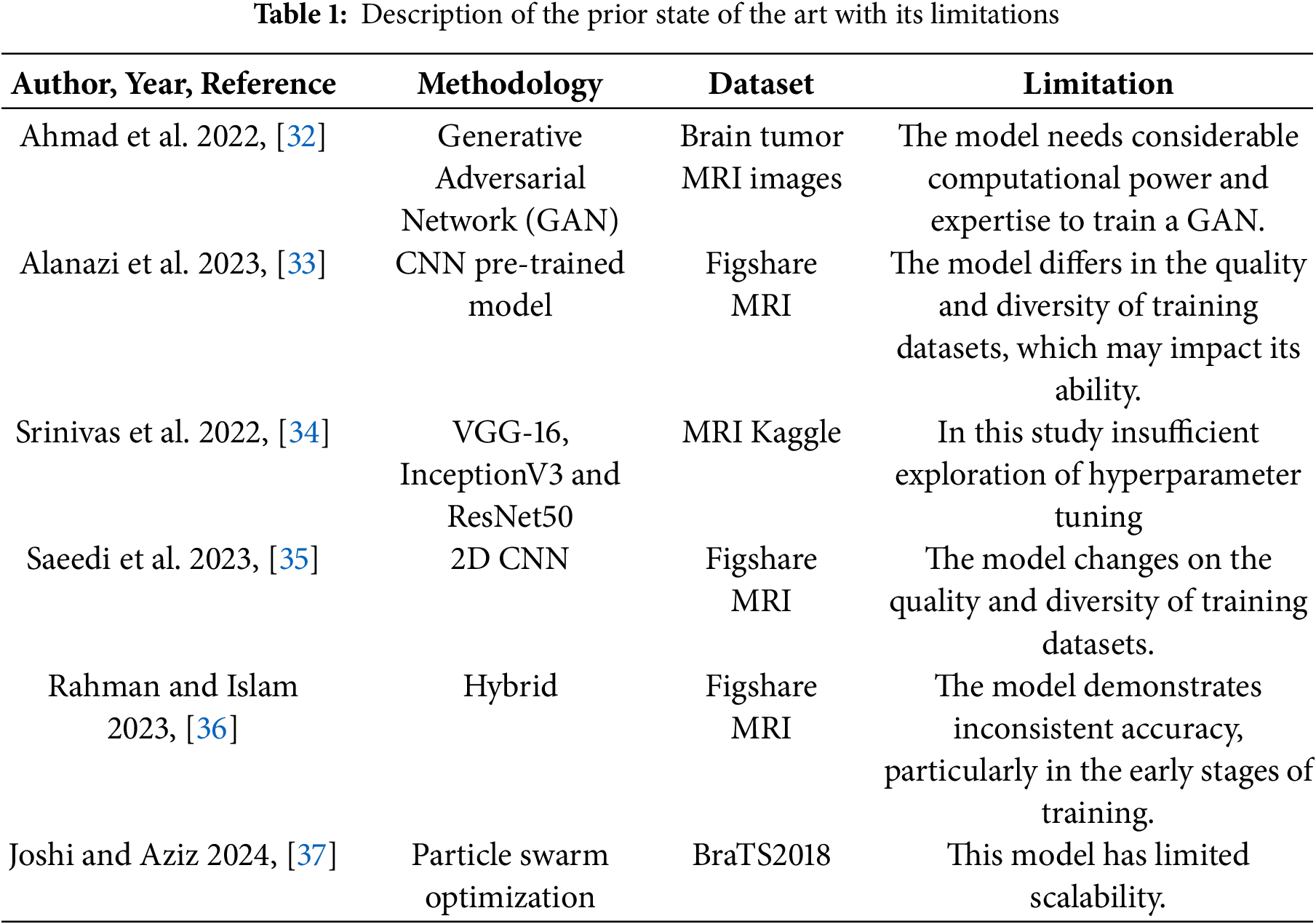
This research demonstrates that most current models do not generalize well and often fail to achieve high accuracy in brain tumor classification, making this a challenging problem. We developed a deep learning framework to assist doctors in detecting brain tumors more accurately, a deep convolutional neural network (DCNN) framework with EfficientNet-B6 as the base architecture, along with customized layers for three-class brain tumor classification, which is shown to achieve better performance in classifying the types of brain tumors than previous models. We provide a detailed comparison to prior studies to validate the effectiveness of our approach.
This section provides the methodology, including dataset collection, data augmentation, and the proposed model. The pre-trained models EfficientNet, InceptionV3, ResNet50, AlexNet, VGG19, and MobileNetV2 are chosen for their efficiency and reliability, as they can extract fine features of the image, which are crucial for the detection of brain tumors. Transfer learning and fine-tuning are applied to optimize the model performance with multiple hyperparameters, and optimizers like Adam are used to reduce loss and increase accuracy by updating learning rates and biases. The categorical cross-entropy loss function is applied to reduce the prediction errors.
The proposed model was trained and evaluated using the Figshare brain MRI dataset introduced by Cheng et al. [38]. This dataset contains 3065 MRI slices from 233 patients and was selected for evaluation since it is commonly used in related studies for performance comparison. It includes three categories of brain tumors: pituitary (931 samples), meningioma (708 samples), and glioma (1426 samples). We additionally validated the proposed Fine-Tuned EfficientNet-B6 model on a private MRI brain tumor dataset to further evaluate its robustness and generalization ability. Fig. 1 presents sample images of custom BT datasets.
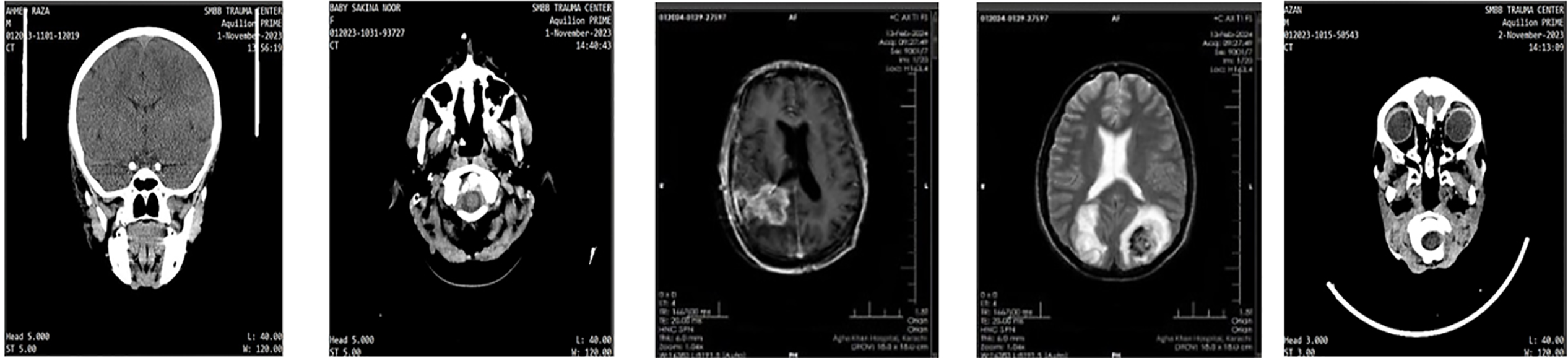
Figure 1: Sample images of the custom BT dataset
The original images are 512 × 512 pixels, but they were resized to 224 × 224 pixels to enhance model performance. As the dataset contains irrelevant areas, background noise, and some missing values, preprocessing was applied. To reduce noise, the Total Variation (TV) filtering method [39] was used, which is a widely adopted technique in image restoration for reconstructing images from noisy data. After preprocessing, the images primarily focused on the central brain region. For the experiments, 80% of the dataset was used for training, and the remaining 20% was used for testing.
Data augmentation methods are used to enlarge the training dataset artificially. Data augmentation is the process of generating new training examples by making random adjustments to the presented images [40]. This technique helps the model learn more effectively and become better equipped to handle diverse, unseen data. As shown in Fig. 2, we used the following methods to present randomly sheared images between −10% and 10%, shifted images horizontally and vertically within a range of −15% to 15%, and zoomed images within 70% to 90% of their original size.
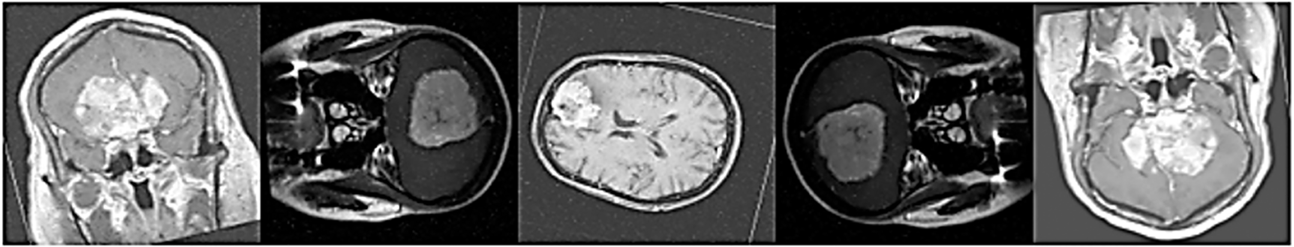
Figure 2: Sample images of MRI after applying the data augmentation approach
This study focused on developing a customized EfficientNetB6 model for multiclass brain tumor classification. Several deep learning models, such as InceptionV3, ResNet50, AlexNet, VGG19, MobileNetV2, and EfficientNet (B0 to B7), were tested on the dataset. EfficientNetB6 achieved the highest accuracy during both training and validation compared to the other models. To further enhance accuracy, the EfficientNetB6 model was customized and fine-tuned layers with the FastNlMeans denoising color filter were also employed to increase the quality of images and minimize noise. Additionally, to enhance computational efficiency, unnecessary boundaries were removed by cropping the images.
3.4 Visual Geometry Group (VGG) Model
VGG is a renowned CNN broadly employed for image detection and classification applications. VGG19 architecture can learn and analyze complicated visual aspects since it consists of 19 layers, 16 convolutional layers, and 3 fully connected layers [40]
MobileNetV2 is built based on MobileNetV1.MobileNetv2 is adapted for small devices such as mobile and embedded devices. It uses depth-wise separable depth-wise separable convolutions to improve computing efficiency. It consists of two new elements: linear bottlenecks and inverted residuals. MobilNetV2 is perfect for real-time applications since it can be used for segmentation, object identification, and picture classification [41].
ResNet50 is a deep convolutional neural network, together with various residual learning frameworks [42]. These residual blocks consist of three convolutional layers, ordered as 1 × 1, 3 × 3, and 7 × 7. ResNet50 architecture is based on 50 layers. These layers provide successful feature extraction, dimensionality reduction, and information preservation through skip connections. Inception v3 is used for image classification applications and grows upon previous models from the Inception family. The use of factorized 7 × 7 convolutions lowers computing costs while preserving excellent accuracy [43]. DenseNet201 is based on a dense connectivity pattern where each layer takes input from all preceding layers. DenseNet201 is a CNN with a unique architecture that addresses typical problems, such as the vanishing gradient problem and inefficiency [44].
EfficientNet has models (B0–B7), and the goal was to increase accuracy over existing convolutional neural network models using fewer machines and parameters [45]. The key advantage of EfficientNet is that it scales the network efficiently using a compound scaling method that optimizes depth, width, and resolution. Depth scaling changes the number of layers; width scaling changes the number of channels in each layer; resolution scaling changes the number of pixels to capture finer detail from images, which aids in recognizing higher-level visual features. The operation of this layer is described by Eq. (1).
X represents a tensor with dimensions corresponding to the height (H) and width (W), which together define the spatial dimensions. The symbol ∑ denotes the summation operation, where indices i, j, and c indicate the positions and channels within the key feature map in the channel.
In this context, in Eq. (2), Z is the output of W and X, which stand for the weight matrix and input vector multiplied by one another. In contrast, b represents the bias vector that is elementwise added to the output of the multiplication of the input vector and the weight. Y is the activation function in Eq. (3).
here, ReLU employed an element-wise weighted sum of Z to give an input present in Eq. (4). Z is passed through a ReLU activation function, where it remains unchanged for positive or zero values, and is set to zero for negative values. The addition of a fully linked output layer follows, where the total number of classes is equal to the number of units.
It is the responsibility of this layer to determine the image’s class. The result is then converted into a probability distribution across the classes using the SoftMax activation function. Eq. (5) shows that SoftMax determines the image’s probability of belonging to each class.
here, exp (Zk) indicates the exponential of the ith element. The exponential value sum for each element in vector Z is represented by
3.8 Customized EfficientNetB6 Model
We experimented with different pre-trained models of CNN, including all versions of EfficientNet, by combining the ReLU activation function with the Softmax layer, the fully connected layer, and the global average pooling layer. After the experiment, we found that EfficientNetB6 gives the best accuracy. However, to further improve prediction and classification results, we decided to enhance the EfficientNetB6 model by adding additional layers. In our method, we first loaded the model’s pre-learned weights after it had been trained on a sizable dataset. The preceding section covered the integration of a global average pooling layer, a fully connected layer with ReLU activation, and a SoftMax output layer. These components were used to train various pre-trained deep learning models, including all versions of EfficientNet. Among these, EfficientNetB6 showed the best performance with higher validation accuracy. Nonetheless, accuracy might still be raised for more precise categorization and forecasting.
As a result, we chose EfficientNetB6 and added more layers to optimize it [46]. Fig. 3 illustrates the EfficientNetB6 model, which consists of seven blocks. Each block contains a different number of mobile inverted bottleneck convolutions (MBConv) with varying filter sizes, strides, and channels. The model uses a compound scaling technique that adjusts depth, width, and resolution to balance model size, accuracy, and computational efficiency, all while maintaining an optimized structure. The Eq. (6) presents Depth, Eq. (7) Width, and Eq. (8) Resolution describe the mathematical computations underlying compound scaling.
here, phi (
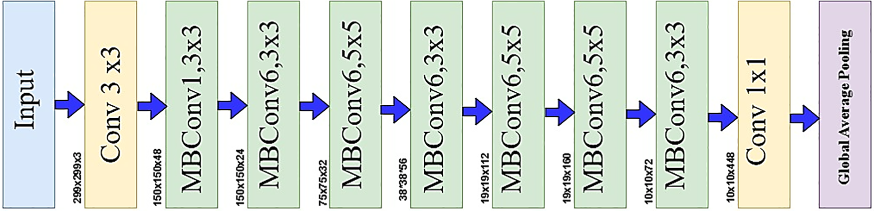
Figure 3: EfficientNetB6 model architecture
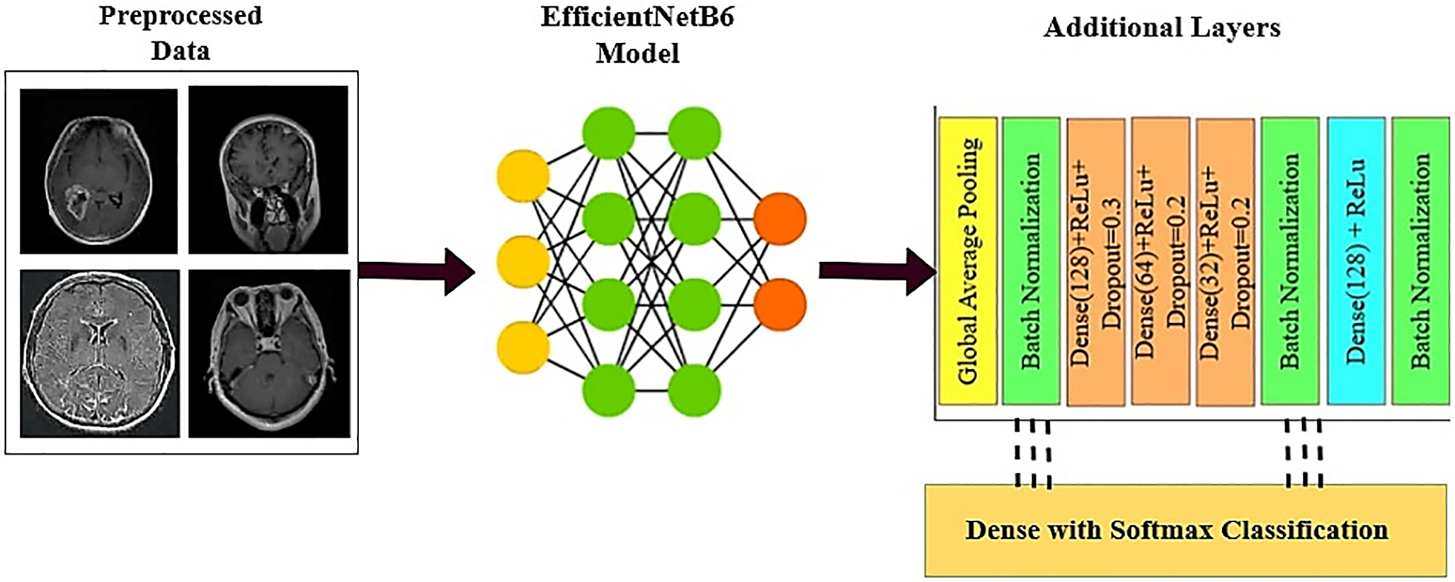
Figure 4: Customized EfficientB6 model
This procedure accelerates convergence during training, improves model stability, and lessens internal covariate movements. The first mini batch mean and variance were presented in Eqs. (9) and (10), respectively.
here,
here
This method uses backpropagation to update β and γ as learnable parameters during training. Each layer’s scaling and shifting are optimized. In addition, three dense layers were incorporated, each with varying numbers of units, ReLU activation, and dropout, as outlined in the configuration. The initial dense layer consists of 128 units, employs ReLU activation, and includes a dropout rate of 0.3. The subsequent dense layer contains 64 units, also uses ReLU activation, and has a dropout rate of 0.2. The third dense layer has 32 units with ReLU activation and a dropout rate of 0.2. As previously mentioned, Eq. (4) illustrates the ReLU function. To assist the network in acquiring more generic and dependable characteristics, the dropout layer randomly turns off certain neurons during training, preventing overfitting [4]. A binary mask is created where probability p is selected for each element randomly. To keep the anticipated value of the activation unchanged, the output is adjusted. The Eqs. (13) and (14) present the dropout works.
In this case, M stands for the dropout mask, and the Bernoulli distribution is expressed as P (X = x).
The tensor values are represented by X in the equation, the dropout rate by p, and the output by Y, following the application of the dropout layer as present in Eq. (15). The network activations are then normalized using batch normalization [48]. To capture more complicated characteristics, a dense layer with 128 units and ReLU activation is used. These features are then sent via a second batch normalization layer. The normalized output is fed into the final output layer, which employs a SoftMax classifier. This classifier categorizes the brain tumor into one of the following classes: glioma, meningioma, pituitary, or no tumor. Fig. 5 presents the proposed model architecture.
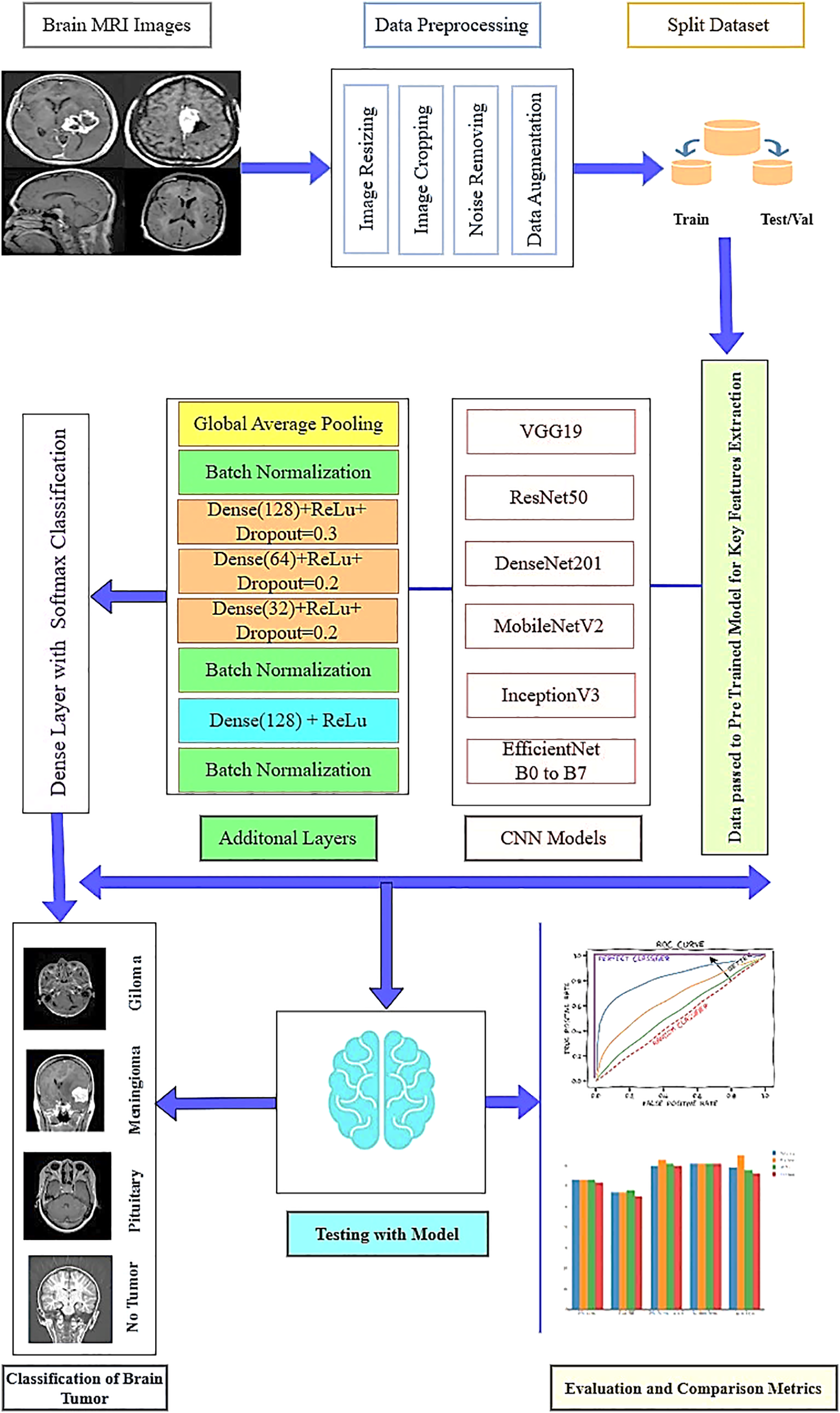
Figure 5: The proposed model architecture
3.9 Grad-Cam Visualization and K-Fold cross Validation
A suitable method for creating a visual justification for choices made by CNN-pretrained models, thereby improving their interpretability, is Grad-CAM visualization. This method generates a heatmap according to the gradients of the target class about the feature mappings of the final convolutional layer [49]. A method for assessing the model’s performance using fresh data is K-fold cross-validation. It aids in forecasting the model’s accuracy in certain applications.
This section describes the experimental performance of the brain tumors that were identified and categorized in this investigation. To enhance the model’s performance in unbalanced and sparse data, various augmentation techniques are implemented. The tools and software needed for model evaluation and training are also provided. This section concludes with a discussion of how to optimize the model’s hyperparameters. This research model was evaluated using a modified EfficientNetB6 architecture, constructed with Python, TensorFlow, and Keras, on a publicly accessible dataset. The research system consists of an Intel Core i7-13700K CPU operating at 3.4 GHz, 32 GB of RAM, a 1 TB SSD, and an NVIDIA GeForce RTX 4060 GPU. While the EfficientNet-B6 model took a slightly longer time to train (approximately 2.8 h per fold) and required more GPU resources than the smaller versions, it consistently achieved higher predictive accuracy (99.10%) at an acceptable computational cost, while the EfficientNet-B0–B4 models trained more quickly but had relatively lower accuracies (96.8%–98.4%). The revised Results and Discussion section now includes this comparative evaluation, showing that the EfficientNet-B6 model provides an optimal trade-off between computational efficiency and model performance that makes it suitable for practical implementation.
4.1 Hyperparameter Optimization
In this section, we will discuss hyperparameter optimization that optimizes the deep learning model for classification tasks [50], such as the optimizer, learning rate, batch size, loss function, and training epochs to improve the accuracy and efficiency of the model. For instance, Grid Search is a popular method that exhaustively searches a predefined set of hyperparameter values [51]; however, it can become computationally expensive with a high number of parameters, whereas Random Search selects hyperparameter combinations randomly, which can result in inconsistent results. Bayesian Optimization has also been shown to perform better than Grid Search in previous studies. In 50 iterations, Bayesian Optimization finds the ideal hyperparameters by using a surrogate model to approximate the objective function. The number of dense layer units, dropout rate, optimizer type, learning rate, and batch size were among the hyperparameters optimized for this investigation. All of the hyperparameters are listed in Table 2.
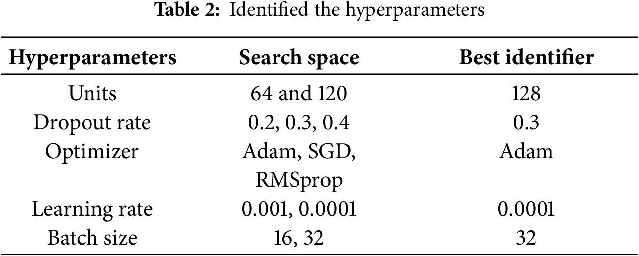
After 50 iterations of Bayesian Optimization, the best hyperparameters were found with the primary objective of minimizing loss because a lower loss value indicates a better-performing model, and categorical cross-entropy was used for the loss function to measure the discrepancy between expected and predicted values. An Adam optimizer was used to update the weights and was initialized with a learning rate of 0.0001, which was fine-tuned to improve performance. The Adam optimizer is relatively simple, uses minimal memory, and converges quickly, which makes it suitable for deep learning for medical imaging analysis compared to other optimizers such as RMSProp, SGD, and Adam etc. Early stopping was not used during training, and the model that produced the best results was chosen for further fine-tuning. We tried freezing the base model layers and training the model with the chosen hyperparameters and additional layers, which resulted in poor performance because the model, trained on a large dataset, could not adapt to the new dataset; instead, we retrained the entire model with a combination of pre-trained and custom layers after unfreezing the layers. For the EfficientNetB6 model, dense layers, dropout, batch normalization, and a global average pooling layer were added; the global average pooling layer simplifies the feature map and accelerates training while minimizing memory requirements. To increase training stability and lessen the likelihood of gradients over-flowing or vanishing, batch normalization was employed. Dropout layers made the model more resilient by preventing overfitting, while dense layers improved the model’s ability to adjust to the task by capturing complex patterns and correlations. By using these fine-tuning techniques, we were able to achieve better results.
4.2 Performance Evaluation Metrics
A confusion matrix (CM), which is arranged as a square grid with rows and columns corresponding to actual and predicted labels, respectively, and records both correct and incorrect classifications for each class, is a table that is typically used to describe how well a trained model performs with test data. The precision of positive predictions is determined by dividing the number of genuine positives by the total number of anticipated positives. The percentage of actual positive samples that the model detects as positive is known as sensitivity, or the true positive rate (TPR). True Positive Rate, or Sensitivity, is the number of true positives divided by the number of positives. True Negative Rate, or Specificity, is the number of true negatives divided by the number of negatives. F1-score (also referred to as the F-measure) is the harmonic meaning between precision and recall.
In this section, the performance of the proposed modified EfficientNetB6 model is compared to that of other deep learning models, including several variants of EfficientNet, as presented in Table 3. The results show that DenseNet201 had the best performance with an accuracy of 80.32%, precision of 80.32%, recall of 80.32%, F1-score of 80.32%, and specificity of 80.32%, while VGG19 had the worst results with an accuracy of 68.40%. The other models, MobileNetV2, ResNet50, and InceptionV3, demonstrated intermediate performance with accuracies of 75.54% and 76.20%, respectively.
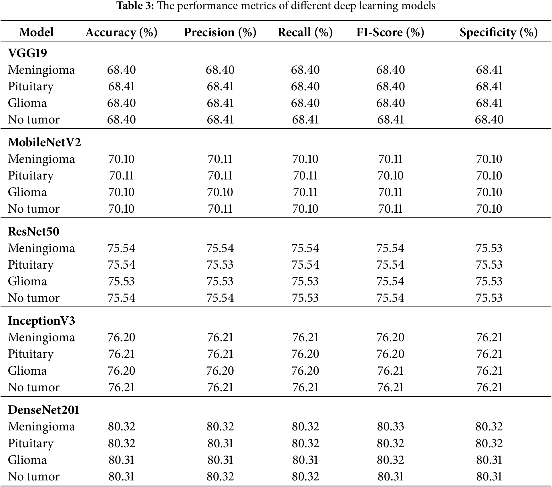
Table 4 summarizes the comparative results of the various EfficientNet architectures tested. Among the tested models, EfficientNetB6 achieved the best performance, with an accuracy, precision, recall, F1-score, and specificity of 94.23%, 94.23%, 94.24%, 94.24%, and 94.24%, respectively, indicating its strong capability of distinguishing positive and negative samples, followed by EfficientNetB5 and EfficientNetB7, which achieved 90% or higher in all evaluation measures, and earlier models such as EfficientNet1, EfficientNetB2, EfficientNetB3, and EfficientNetB4 which showed comparatively lower but gradually improving results as network depth and scaling increased. Overall, the results indicate that the newer versions (B5–B7), especially EfficientNetB6, deliver significant improvements in predictive accuracy over the original versions. The results for the Fine-Tuned EfficientNetB6 model for brain tumor multiclass classification are shown in Table 5, which demonstrates that the model produced highly consistent results for all classes (Meningioma, Pituitary, Glioma, and No Tumor) with accuracy, precision, recall, F1-score, and specificity values between 99.10% and 99.11%, which further indicates the robust generalization and reliability of the model in accurately classifying brain tumor types with virtually no misclassification. Fig. 6 illustrates the learning curve of the proposed method. The accuracy of training and validation is shown in the left sub-image, while the loss of training and validation is shown in the right sub-image. These curves provide a clear picture of the model’s learning process and error dynamics, making them essential for performance analysis.
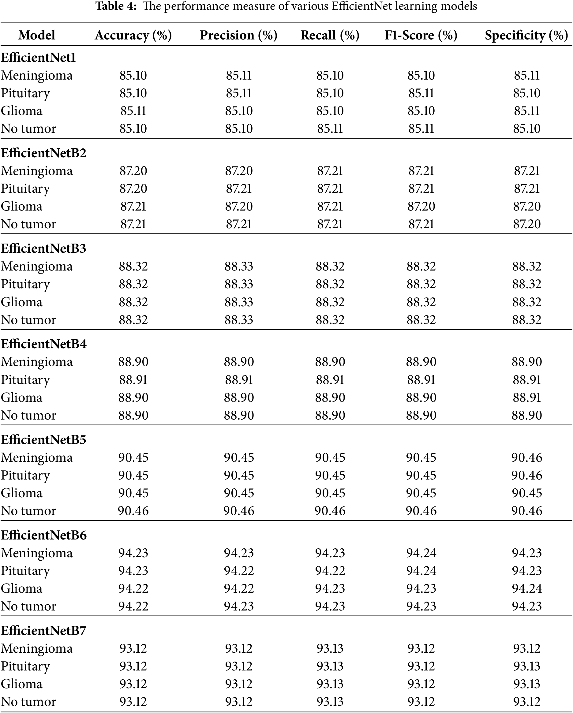
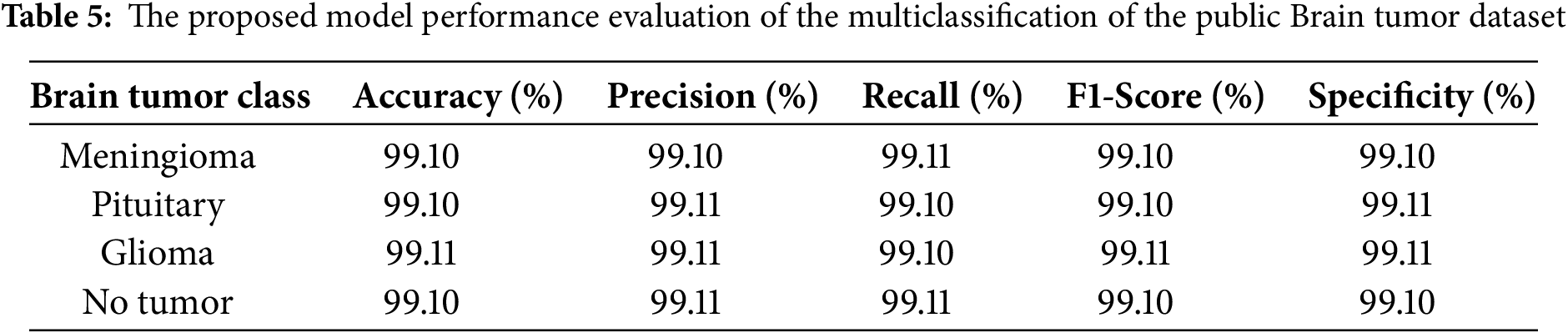
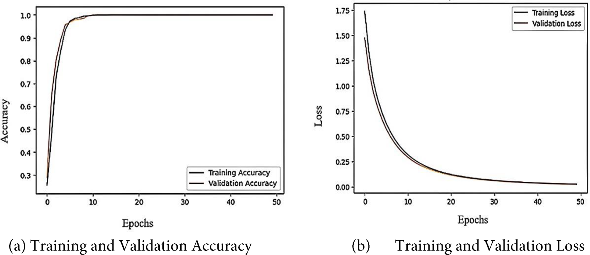
Figure 6: The accuracy and loss learning curves of the proposed model
The suggested Fine-Tuned EfficientNet-B6 model performs marginally better on the public brain tumour dataset than on the custom dataset, according to a comparison of the findings in Tables 5 and 6. The model consistently scores between 99.10% and 99.11% in accuracy, precision, recall, F1-score, and specificity across all four classes (Meningioma, Pituitary, Glioma, and No Tumour), as shown in Table 5. On the other hand, Table 6 shows that, although still good, the model’s performance on the custom data set falls between 97.8% and 97.9% for most assessment measures. The results show that the model retains strong generalization and dependable classification power across both datasets, despite this slight decline, proving its efficacy in multiclass brain tumor identification.
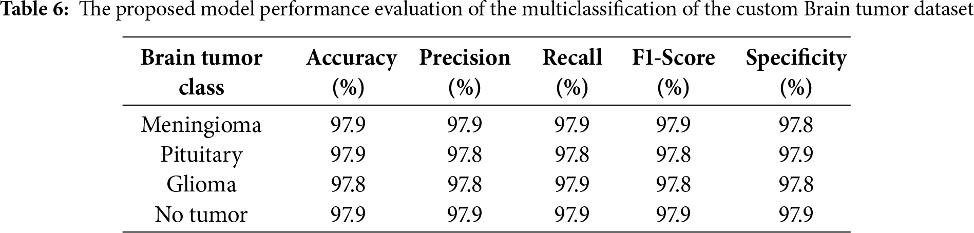
Fig. 7 shows the confusion matrix for the four forms of brain tumors with the values for each tumor type: true positive (TP), true negative (TN), false positive (FP), and false negative (FN) for meningioma (TP = 149, TN = 408, FP = 9, and FN = 3), for the pituitary tumor class (TP = 99, TN = 456, FP = 7, and FN = 7), for Glioma tumors (TP = 150, TN = 403, FP = 6, and FN = 10), and for the No-tumor class (TP = 145, TN = 414, FP = 4, and FN = 6). Using these values, we calculated several performance metrics to show that our proposed model betters the other methods reviewed in the research. Fig. 8 shows the ROC curve of the proposed model, which plots the true positive rate against the false positive rate.
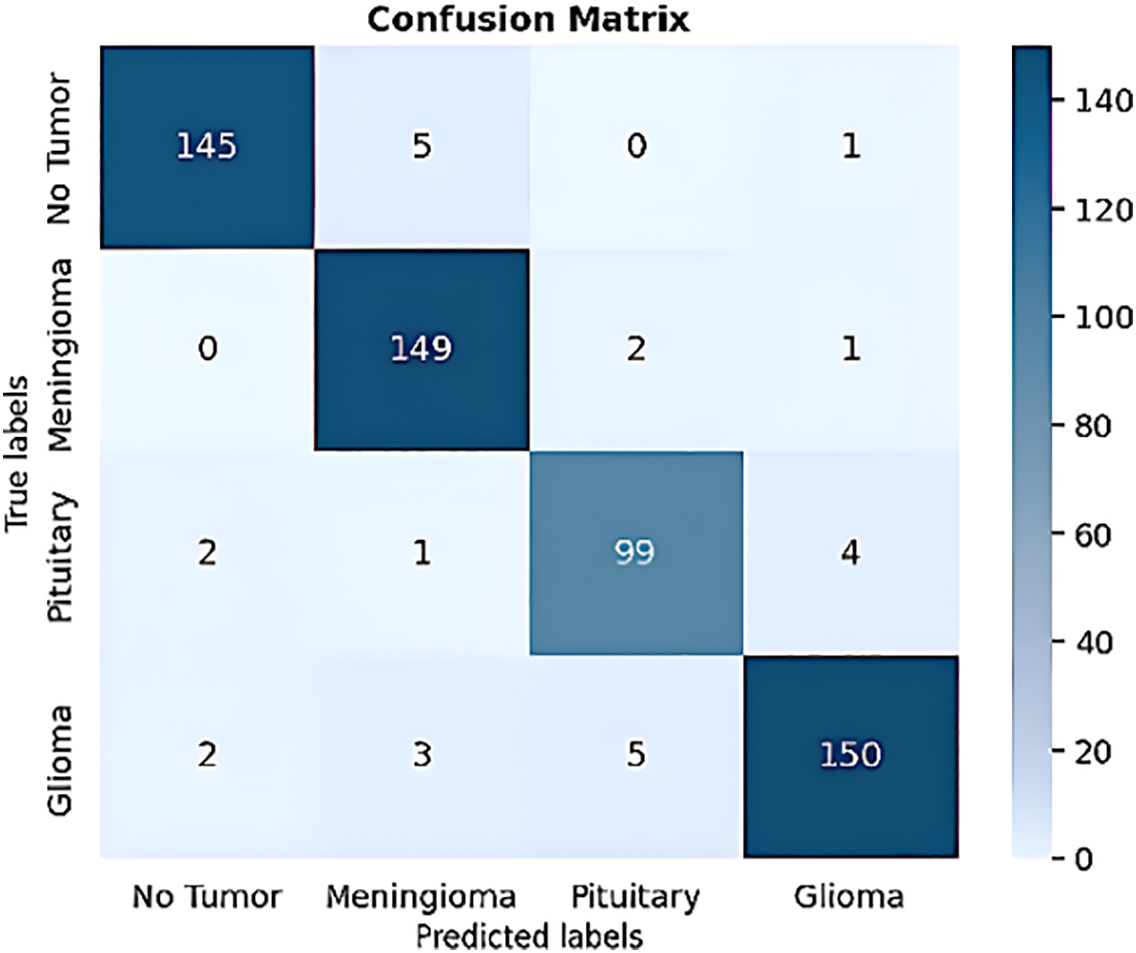
Figure 7: The proposed model confusion matrix
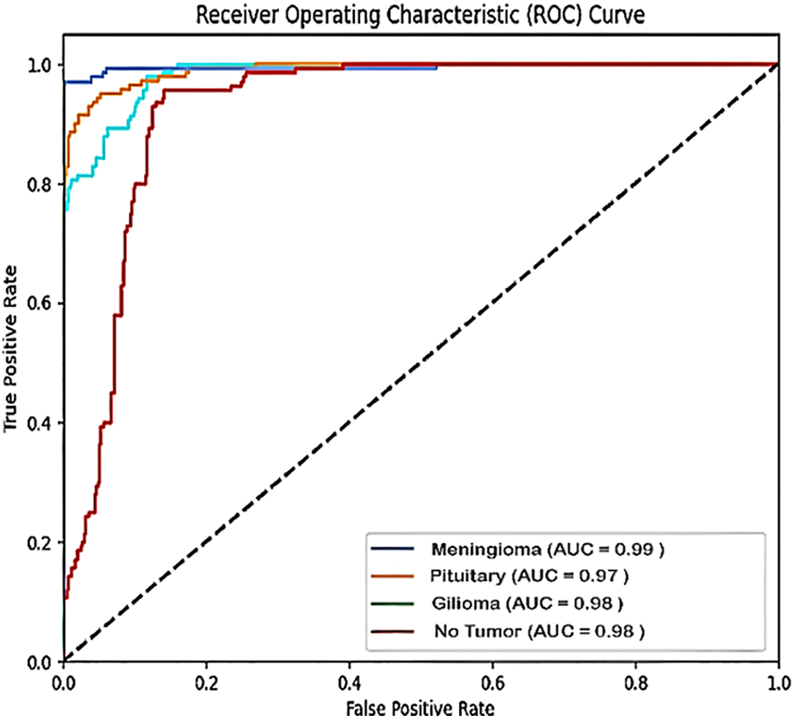
Figure 8: The proposed model ROC curve
Ablation Study
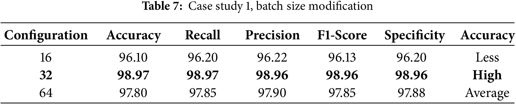
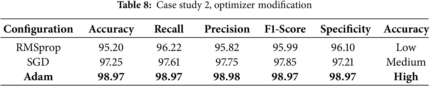
An ablation study was conducted to investigate the effect of various components and hyperparameters on the proposed model. For example, in case study 1, the effect of changing the batch size (16, 32, 64) on the model performance of each batch size was evaluated by computing the corresponding performance metrics for each batch size, which showed that batch sizes of 32 and 64 produced the same high accuracy, whereas a batch size of 16 resulted in a decrease in accuracy (see Table 7). Two different optimizers, Adam, SGD, and RMSprop, were applied to train the model, and the performance of each optimizer was evaluated to identify the most suitable one for this task (see Table 8).
In case study 3, we tested learning rates of 0.01, 0.001, and 0.0001 to identify the most effective learning rate for training the model. The results are shown in Table 9. The ablation study highlights that each component and hyperparameter is crucial to the performance of the EfficientNetB4 model. To evaluate our model performance and prevent overfitting. We conducted K-Fold Cross-Validation using a 5-fold. The model was trained and verified five times on five subsets of the dataset. Every time, a distinct subset is used for validation. Results are presented in Table 10. The K-Fold cross-validation results show that the model performs consistently across various dataset splits, achieving high accuracy and low loss, which highlights its reliability and strong generalization capabilities.
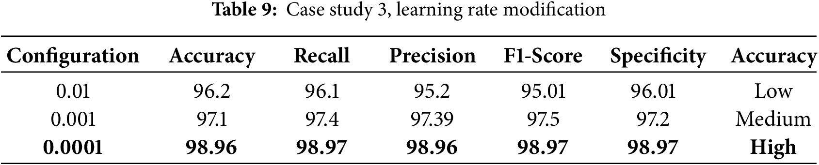
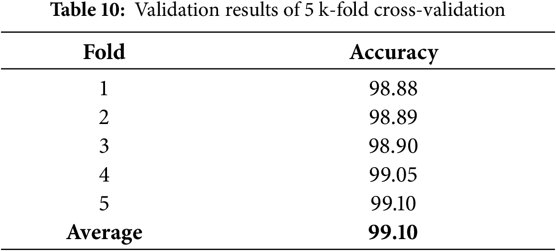
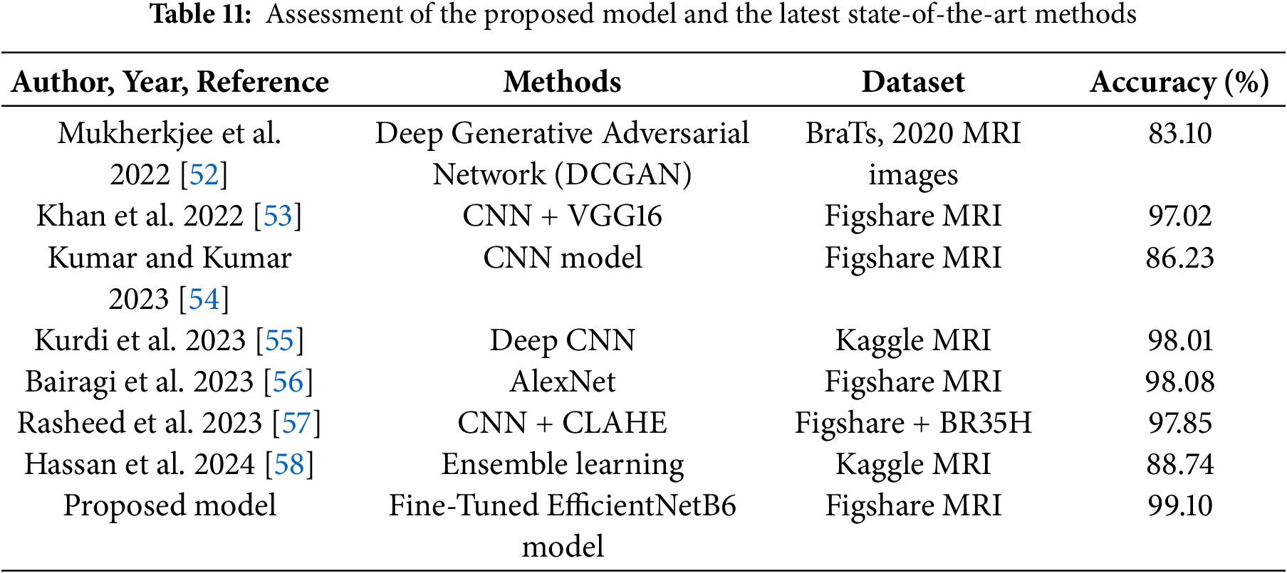
Table 11 presents the performance of our model alongside other recent studies that used ML and DL for brain tumor detection. Since preprocessing, training methods, and resources differ across studies, a direct comparison is not possible. Nevertheless, our model achieved excellent results, with an overall accuracy of 99.10%.
The proposed deep learning model employs Gradient-weighted Class Activation Mapping (Grad-CAM) as a visualization approach to enhance the interpretability of road anomaly categorization. Grad-CAM creates a coarse localization map by using the gradients of the model’s output that correspond to a target class and sending them back to the last convolutional layer. The areas of the image that are most pertinent to the model’s decision-making process are highlighted in this map. The last convolutional layer captures high-level semantic information and is essential for precise categorization. The creation of heatmaps by Grad-CAM highlights these crucial regions, increasing transparency and promoting confidence in automated systems. Fig. 9 illustrates the Grad-CAM visualization of the proposed model.
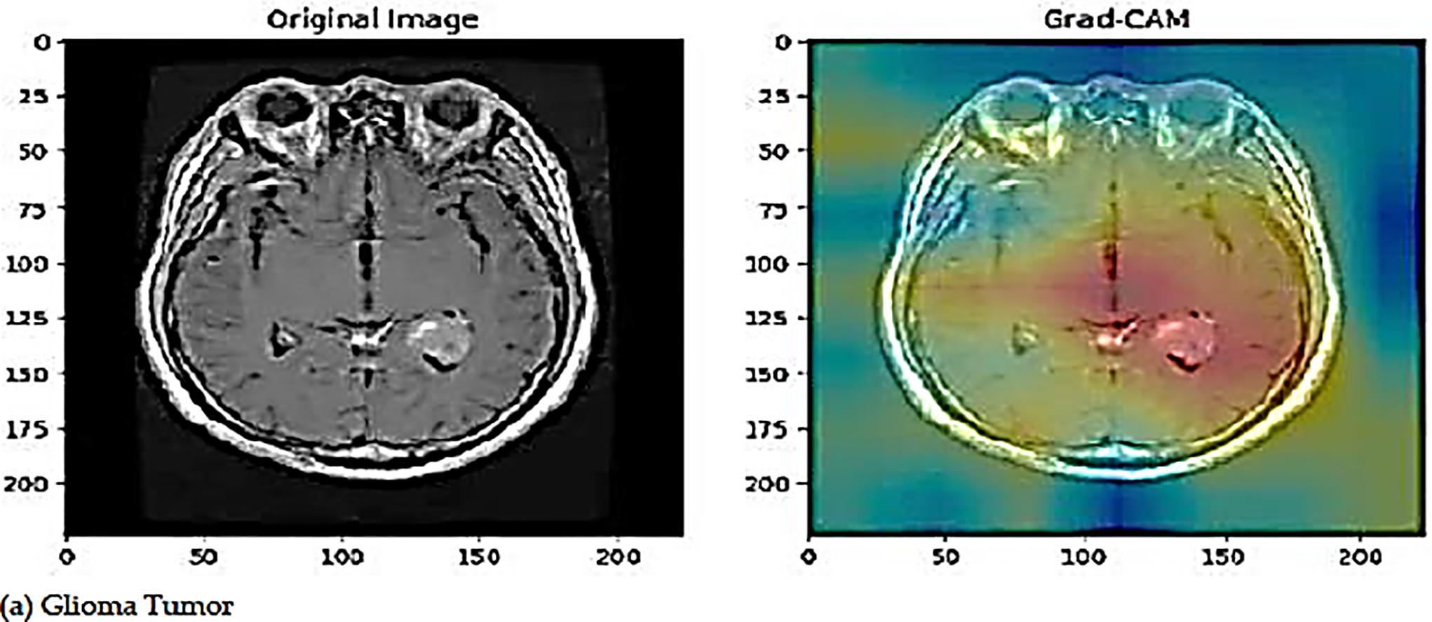
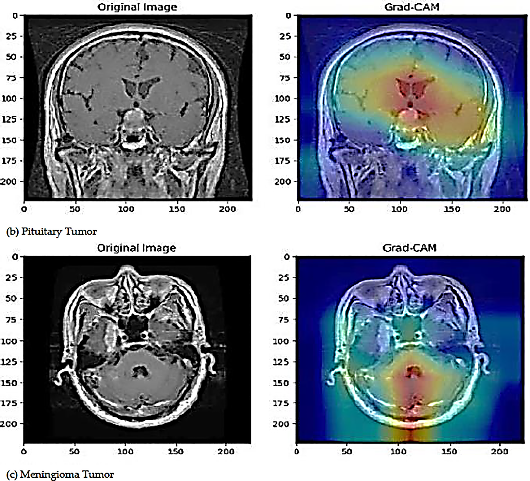
Figure 9: The visualization of original images and Grad-CAM images
6 Conclusion and Future Direction
Brain tumors are a critical health concern, and manual diagnosis is both time-consuming and highly dependent on the expertise of specialists. The development of automated diagnostic systems is of great importance. This study presents a fine-tuned deep learning model based on EfficientNet-B6 for the detection of brain tumors using MRI images. The effectiveness and dependability of the suggested framework were demonstrated by its 99.10% accuracy. Several different convolutional neural network (CNN) designs, in conjunction with transfer learning techniques, were also assessed for comparison. Although the outcomes are encouraging, further development is still needed. However, this study’s model was trained and tested on a proprietary MRI dataset, which may limit its applicability to broader or more diverse clinical populations. Furthermore, multi-modal imaging or patient clinical data, which could further enhance diagnostic performance, are not yet included in the framework. In the future, we aim to explore more advanced deep CNN architectures for brain tumor classification and present segmentation techniques with reduced computational cost. Additionally, the dataset will be enriched with a larger number of MRI scans to improve model accuracy further. Beyond MRI, the proposed approach will also be extended to other medical imaging modalities such as X-ray, computed tomography (CT), and ultrasound, creating opportunities for broader applications in medical image analysis and future research.
Acknowledgement: The authors are grateful to King Saud University, Riyadh, Saudi Arabia, for funding this work through the Researchers Supporting Research Funding program (ORF-2025-1268).
Funding Statement: This work was funded by the King Saud University, Riyadh, Saudi Arabia, for funding this work through the Researchers Supporting Research Funding program, (ORF-2025-1268).
Author Contributions: Conceptualization, Mohammad Siraj and Sarfaraz Abdul Sattar Natha; methodology, Sarfaraz Abdul Sattar Natha and Maqsood Mahmud; software, Majid Altamimi and Adamali Shah; validation, Adamali Shah and Sarfaraz Abdul Sattar Natha; formal analysis, Mohammad Siraj and Maqsood Mahmud; investigation, Maqsood Mahmud and Majid Altamimi; resources, Mohammad Siraj and Sarfaraz Abdul Sattar Natha; data curation, Sarfaraz Abdul Sattar Natha; writing—original draft preparation, Sarfaraz Abdul Sattar Natha and Maqsood Mahmud; writing—review and editing, Mohammad Siraj, Majid Altamimi, Adamali Shah and Maqsood Mahmud; visualization, Mohammad Siraj and Sarfaraz Abdul Sattar Natha; supervision, Mohammad Siraj, Maqsood Mahmud and Sarfaraz Abdul Sattar Natha; project administration, Adamali Shah, Maqsood Mahmud and Majid Altamimi; funding acquisition, Mohammad Siraj, Adamali Shah and Majid Altamimi. All authors reviewed the results and approved the final version of the manuscript.
Availability of Data and Materials: The datasets are publicly available MRI images of brain tumor datasets https://figshare.com/articles/dataset/brain_tumor_dataset/1512427 (accessed on 15 January 2025).
Ethics Approval: Not applicable.
Conflicts of Interest: The authors declare no conflicts of interest to report regarding the present study.
References
1. Louis DN, Perry A, Reifenberger G, von Deimling A, Figarella-Branger D, Cavenee WK, et al. The 2016 World Health Organization classification of tumors of the central nervous system: a summary. Acta Neuropathol. 2016;131(6):803–20. doi:10.1007/s00401-016-1545-1. [Google Scholar] [PubMed] [CrossRef]
2. Swati ZNK, Zhao Q, Kabir M, Ali F, Ali Z, Ahmed S, et al. Content-based brain tumor retrieval for MR images using transfer learning. IEEE Access. 2019;7:17809–22. doi:10.1109/ACCESS.2019.2892455. [Google Scholar] [CrossRef]
3. Soni N, Ora M, Bathla G, Szekeres D, Desai A, Pillai JJ, et al. Meningioma: molecular updates from the 2021 World Health Organization classification of CNS tumors and imaging correlates. AJNR Am J Neuroradiol. 2025;46(2):240–50. doi:10.3174/ajnr.a8368. [Google Scholar] [PubMed] [CrossRef]
4. Dayarathna S, Islam KT, Uribe S, Yang G, Hayat M, Chen Z. Deep learning based synthesis of MRI, CT and PET: review and analysis. Med Image Anal. 2024;92(6003):103046. doi:10.1016/j.media.2023.103046. [Google Scholar] [PubMed] [CrossRef]
5. Pal D, Reddy PB, Roy S. Attention UW-Net: a fully connected model for automatic segmentation and annotation of chest X-ray. Comput Biol Med. 2022;150(6):106083. doi:10.1016/j.compbiomed.2022.106083. [Google Scholar] [PubMed] [CrossRef]
6. Heckel R, Jacob M, Chaudhari A, Perlman O, Shimron E. Deep learning for accelerated and robust MRI reconstruction. Magn Reson Mater Phys Biol Med. 2024;37(3):335–68. doi:10.1007/s10334-024-01173-8. [Google Scholar] [PubMed] [CrossRef]
7. Natha S, Laila U, Gashim IA, Mahboob K, Saeed MN, Noaman KM. Automated brain tumor identification in biomedical radiology images: a multi-model ensemble deep learning approach. Appl Sci. 2024;14(5):2210. doi:10.3390/app14052210. [Google Scholar] [CrossRef]
8. Alharbe N, Almalki M. IoT-enabled healthcare transformation leveraging deep learning for advanced patient monitoring and diagnosis. Multimed Tools Appl. 2025;84(19):21331–44. doi:10.1007/s11042-024-19919-w. [Google Scholar] [CrossRef]
9. Ahmad S, Ullah T, Ahmad I, Al-Sharabi A, Ullah K, Khan RA, et al. A novel hybrid deep learning model for metastatic cancer detection. Comput Intell Neurosci. 2022;2022(11):8141530. doi:10.1155/2022/8141530. [Google Scholar] [PubMed] [CrossRef]
10. Khalighi S, Reddy K, Midya A, Pandav KB, Madabhushi A, Abedalthagafi M. Artificial intelligence in neuro-oncology: advances and challenges in brain tumor diagnosis, prognosis, and precision treatment. npj Precis Oncol. 2024;8(1):80. doi:10.1038/s41698-024-00575-0. [Google Scholar] [PubMed] [CrossRef]
11. Cekic E, Pinar E, Pinar M, Dagcinar A. Deep learning-assisted segmentation and classification of brain tumor types on magnetic resonance and surgical microscope images. World Neurosurg. 2024;182:e196–204. doi:10.1016/j.wneu.2023.11.073. [Google Scholar] [PubMed] [CrossRef]
12. Rudnicka Z, Szczepanski J, Pregowska A. Artificial intelligence-based algorithms in medical image scan segmentation and intelligent visual content generation—a concise overview. Electronics. 2024;13(4):746. doi:10.3390/electronics13040746. [Google Scholar] [CrossRef]
13. Abou Ali M, Charafeddine J, Dornaika F, Arganda-Carreras I. Enhancing generalization and mitigating overfitting in deep learning for brain cancer diagnosis from MRI. Appl Magn Reson. 2025;56(3):359–94. doi:10.1007/s00723-024-01743-y. [Google Scholar] [CrossRef]
14. Gayap HT, Akhloufi MA. Deep machine learning for medical diagnosis, application to lung cancer detection: a review. BioMedInformatics. 2024;4(1):236–84. doi:10.3390/biomedinformatics4010015. [Google Scholar] [CrossRef]
15. Thaiparnit S, Janchidfah T, Farooq A. Brain tumor classification system using decision tree algorithm. In: 2025 IEEE International Conference on Cybernetics and Innovations (ICCI); 2025 Apr 2–4; Chonburi, Thailand. Piscataway, NJ, USA: IEEE; 2025. p. 1–6. doi:10.1109/ICCI64209.2025.10987380. [Google Scholar] [CrossRef]
16. Zaw HT, Maneerat N, Win KY. Brain tumor detection based on Naïve Bayes classification. In: 2019 5th International Conference on Engineering, Applied Sciences and Technology (ICEAST); 2019 Jul 2–5; Luang Prabang, Laos. Piscataway, NJ, USA: IEEE; 2019. p. 1–4. doi:10.1109/iceast.2019.8802562. [Google Scholar] [CrossRef]
17. Abdullah N, Ngah UK, Aziz SA. Image classification of brain MRI using support vector machine. In: 2011 IEEE International Conference on Imaging Systems and Techniques (IST 2011); 2011 May 17–18; Batu Ferringhi, Malaysia. Piscataway, NJ, USA: IEEE; 2011. p. 242–7. doi:10.1109/IST.2011.5962185. [Google Scholar] [CrossRef]
18. Venkata Subbarao M, Sudheer Kumar T, Chowdary PSR, Chakravarthy VVSSS. Brain tumor classification using decision tree and neural network classifiers. In: Data engineering and intelligent computing. Singapore: Springer Nature Singapore; 2022. p. 405–12. doi:10.1007/978-981-19-1559-8_41. [Google Scholar] [CrossRef]
19. Gautam N, Basu A, Sarkar R. Lung cancer detection from thoracic CT scans using an ensemble of deep learning models. Neural Comput Appl. 2024;36(5):2459–77. doi:10.1007/s00521-023-09130-7. [Google Scholar] [CrossRef]
20. Nemade V, Pathak S, Dubey AK. Deep learning-based ensemble model for classification of breast cancer. Microsyst Technol. 2024;30(5):513–27. doi:10.1007/s00542-023-05469-y. [Google Scholar] [CrossRef]
21. Wu L, Wang S, Liu J, Hou L, Li N, Su F, et al. A survey of MRI-based brain tissue segmentation using deep learning. Complex Intell Syst. 2024;11(1):64. doi:10.1007/s40747-024-01639-1. [Google Scholar] [CrossRef]
22. Li L, Wang X, Ding R, Luo L, Wu Q, He Z. CMS-YOLO: an automated multi-category brain tumor detection algorithm based on improved YOLOv10s. Comput Mater Contin. 2025;85(1):1287–309. doi:10.32604/cmc.2025.065670. [Google Scholar] [CrossRef]
23. Hasan MS, Komol MMR, Fahim F, Islam J, Pervin T, Hasan MM. DEEP Q-NAS: a new algorithm based on neural architecture search and reinforcement learning for brain tumor identification from MRI. Comput Biol Med. 2025;196(1):110767. doi:10.1016/j.compbiomed.2025.110767. [Google Scholar] [PubMed] [CrossRef]
24. Hasan N, Rana MM, Hasan MM, Azad A, Afroz D, Komol MMR, et al. STSA-based early-stage detection of small brain tumors using neural network. Eng Rep. 2025;7(5):e70135. doi:10.1002/eng2.70135. [Google Scholar] [CrossRef]
25. Kavin Kumar K, Dinesh PM, Rayavel P, Vijayaraja L, Dhanasekar R, Kesavan R, et al. Brain tumor identification using data augmentation and transfer learning approach. Comput Syst Sci Eng. 2023;46(2):1845–61. doi:10.32604/csse.2023.033927. [Google Scholar] [CrossRef]
26. Asiri AA, Shaf A, Ali T, Aamir M, Usman A, Irfan M, et al. Multi-level deep generative adversarial networks for brain tumor classification on magnetic resonance images. Intell Autom Soft Comput. 2023;36(1):127–43. doi:10.32604/iasc.2023.032391. [Google Scholar] [CrossRef]
27. Ali Yazdan S, Ahmad R, Iqbal N, Rizwan A, Khan AN, Kim DH. An efficient multi-scale convolutional neural network based multi-class brain MRI classification for SaMD. Tomography. 2022;8(4):1905–27. doi:10.3390/tomography8040161. [Google Scholar] [PubMed] [CrossRef]
28. Özkaraca O, Bağrıaçık Oİ, Gürüler H, Khan F, Hussain J, Khan J, et al. Multiple brain tumor classification with dense CNN architecture using brain MRI images. Life. 2023;13(2):349. doi:10.3390/life13020349. [Google Scholar] [PubMed] [CrossRef]
29. Gómez-Guzmán MA, Jiménez-Beristaín L, García-Guerrero EE, López-Bonilla OR, Tamayo-Perez UJ, Esqueda-Elizondo JJ, et al. Classifying brain tumors on magnetic resonance imaging by using convolutional neural networks. Electronics. 2023;12(4):955. doi:10.3390/electronics12040955. [Google Scholar] [CrossRef]
30. Bodapati JD, Shaik NS, Naralasetti V, Mundukur NB. Joint training of two-channel deep neural network for brain tumor classification. Signal Image Video Process. 2021;15(4):753–60. doi:10.1007/s11760-020-01793-2. [Google Scholar] [CrossRef]
31. Asif S, Zhao M, Chen X, Zhu Y. BMRI-NET: a deep stacked ensemble model for multi-class brain tumor classification from MRI images. Interdiscip Sci. 2023;15(3):499–514. doi:10.1007/s12539-023-00571-1. [Google Scholar] [PubMed] [CrossRef]
32. Ahmad B, Sun J, You Q, Palade V, Mao Z. Brain tumor classification using a combination of variational autoencoders and generative adversarial networks. Biomedicines. 2022;10(2):223. doi:10.3390/biomedicines10020223. [Google Scholar] [PubMed] [CrossRef]
33. Alanazi MF, Ali MU, Hussain SJ, Zafar A, Mohatram M, Irfan M, et al. Brain tumor/mass classification framework using magnetic-resonance-imaging-based isolated and developed transfer deep-learning model. Sensors. 2022;22(1):372. doi:10.3390/s22010372. [Google Scholar] [PubMed] [CrossRef]
34. Srinivas C, Nandini Prasad KS, Zakariah M, Alothaibi YA, Shaukat K, Partibane B, et al. Deep transfer learning approaches in performance analysis of brain tumor classification using MRI images. J Healthc Eng. 2022;2022(2):3264367. doi:10.1155/2022/3264367. [Google Scholar] [PubMed] [CrossRef]
35. Saeedi S, Rezayi S, Keshavarz H, Kalhori SRN. MRI-based brain tumor detection using convolutional deep learning methods and chosen machine learning techniques. BMC Med Inform Decis Mak. 2023;23(1):16. doi:10.1186/s12911-023-02114-6. [Google Scholar] [PubMed] [CrossRef]
36. Rahman T, Islam MS. MRI brain tumor detection and classification using parallel deep convolutional neural networks. Meas Sens. 2023;26(1):100694. doi:10.1016/j.measen.2023.100694. [Google Scholar] [CrossRef]
37. Joshi AA, Aziz RM. Deep learning approach for brain tumor classification using metaheuristic optimization with gene expression data. Int J Imag Syst Technol. 2024;34(2):e23007. doi:10.1002/ima.23007. [Google Scholar] [CrossRef]
38. Cheng J, Huang W, Cao S, Yang R, Yang W, Yun Z, et al. Enhanced performance of brain tumor classification via tumor region augmentation and partition. PLoS One. 2015;10(10):e0140381. doi:10.1371/journal.pone.0140381. [Google Scholar] [PubMed] [CrossRef]
39. Rao KN, Khalaf OI, Krishnasree V, Kumar AS, Alsekait DM, Priyanka SS, et al. An efficient brain tumor detection and classification using pre-trained convolutional neural network models. Heliyon. 2024;10(17):e36773. doi:10.1016/j.heliyon.2024.e36773. [Google Scholar] [PubMed] [CrossRef]
40. Gill KS, Sharma A, Anand V, Gupta R. Brain tumor detection using VGG19 model on Adadelta and SGD optimizer. In: 2022 6th International Conference on Electronics, Communication and Aerospace Technology (ICECA 2022); 2022 Dec 1–3; Coimbatore, India. Piscataway, NJ, USA: IEEE; 2023. p. 1407–12. doi:10.1109/ICECA55336.2022.10009496. [Google Scholar] [CrossRef]
41. Adamu MJ, Kawuwa HB, Qiang L, Nyatega CO, Younis A, Fahad M, et al. Efficient and accurate brain tumor classification using hybrid MobileNetV2-support vector machine for magnetic resonance imaging diagnostics in neoplasms. Brain Sci. 2024;14(12):1178. doi:10.3390/brainsci14121178. [Google Scholar] [PubMed] [CrossRef]
42. Asiri AA, Shaf A, Ali T, Aamir M, Irfan M, Alqahtani S, et al. Brain tumor detection and classification using fine-tuned CNN with ResNet50 and U-Net model: a study on TCGA-LGG and TCIA dataset for MRI applications. Life. 2023;13(7):1449. doi:10.3390/life13071449. [Google Scholar] [PubMed] [CrossRef]
43. Fathima N, Kumar P. Multi-class classification of brain tumours: leveraging VGG, InceptionV3, and DenseNet201 transfer learning. In: 2024 IEEE International Students’ Conference on Electrical, Electronics and Computer Science (SCEECS 2024); 2024 Feb 24–25; Bhopal, India. Piscataway, NJ, USA: IEEE; 2024. p. 1–8. doi:10.1109/SCEECS61402.2024.10482369. [Google Scholar] [CrossRef]
44. Ewees AA, Ismail FH, Labeeb NS, Gaheen MA. Multi-level thresholding segmentation for brain tumor detection using optimized deep learning approach. Neural Comput Appl. 2025;37(23):19279–302. doi:10.1007/s00521-025-11398-w. [Google Scholar] [CrossRef]
45. Al-Sabaawi A, Ibrahim HM, Arkah ZM, Al-Amidie M, Alzubaidi L. Amended convolutional neural network with global average pooling for image classification. In: Intelligent systems design and applications. Berlin/Heidelberg, Germany: Springer; 2021. p. 171–80. doi:10.1007/978-3-030-71187-0_16. [Google Scholar] [CrossRef]
46. Rybczak M, Kozakiewicz K. Deep machine learning of MobileNet, efficient, and inception models. Algorithms. 2024;17(3):96. doi:10.3390/a17030096. [Google Scholar] [CrossRef]
47. Kokkalla S, Kakarla J, Venkateswarlu IB, Singh M. Three-class brain tumor classification using deep dense inception residual network. Soft Comput. 2021;25(13):8721–9. doi:10.1007/s00500-021-05748-8. [Google Scholar] [PubMed] [CrossRef]
48. Hekmat A, Zhang Z, Rehman Khan SU, Bilal O. Brain tumor diagnosis redefined: leveraging image fusion for MRI enhancement classification. Biomed Signal Process Control. 2025;109:108040. doi:10.1016/j.bspc.2025.108040. [Google Scholar] [CrossRef]
49. Ben Said A, Hadjidj R, Foufou S. Total variation for image denoising based on a novel smart edge detector: an application to medical images. J Math Imag Vis. 2019;61(1):106–21. doi:10.1007/s10851-018-0829-6. [Google Scholar] [CrossRef]
50. Biswas A, Bhattacharya P, Maity SP, Banik R. Data augmentation for improved brain tumor segmentation. IETE J Res. 2023;69(5):2772–82. doi:10.1080/03772063.2021.1905562. [Google Scholar] [CrossRef]
51. Lawrence MO. A hybrid bio-inspired augmented with hyper-parameter deep learning model for brain tumor classification. J Electr Syst Inf Technol. 2025;12(1):35. doi:10.1186/s43067-025-00207-y. [Google Scholar] [CrossRef]
52. Mukherkjee D, Saha P, Kaplun D, Sinitca A, Sarkar R. Brain tumor image generation using an aggregation of GAN models with style transfer. Sci Rep. 2022;12(1):9141. doi:10.1038/s41598-022-12646-y. [Google Scholar] [PubMed] [CrossRef]
53. Khan MSI, Rahman A, Debnath T, Karim MR, Nasir MK, Band SS, et al. Accurate brain tumor detection using deep convolutional neural network. Comput Struct Biotechnol J. 2022;20:4733–45. doi:10.1016/j.csbj.2022.08.039. [Google Scholar] [PubMed] [CrossRef]
54. Kumar S, Kumar D. Human brain tumor classification and segmentation using CNN. Multimed Tools Appl. 2023;82(5):7599–620. doi:10.1007/s11042-022-13713-2. [Google Scholar] [CrossRef]
55. Kurdi SZ, Ali MH, Jaber MM, Saba T, Rehman A, Damaševičius R. Brain tumor classification using meta-heuristic optimized convolutional neural networks. J Pers Med. 2023;13(2):181. doi:10.3390/jpm13020181. [Google Scholar] [PubMed] [CrossRef]
56. Bairagi VK, Gumaste PP, Rajput SH, Chethan KS. Automatic brain tumor detection using CNN transfer learning approach. Med Biol Eng Comput. 2023;61(7):1821–36. doi:10.1007/s11517-023-02820-3. [Google Scholar] [PubMed] [CrossRef]
57. Rasheed Z, Ma YK, Ullah I, Ghadi YY, Khan MZ, Khan MA, et al. Brain tumor classification from MRI using image enhancement and convolutional neural network techniques. Brain Sci. 2023;13(9):1320. doi:10.3390/brainsci13091320. [Google Scholar] [PubMed] [CrossRef]
58. Hassan MF, Al-Zurfi AN, Alsalihi MH, Ahmed K. An effective ensemble learning approach for classification of glioma grades based on novel MRI features. Sci Rep. 2024;14(1):11977. doi:10.1038/s41598-024-61444-1. [Google Scholar] [PubMed] [CrossRef]
Cite This Article
 Copyright © 2025 The Author(s). Published by Tech Science Press.
This work is licensed under a Creative Commons Attribution 4.0 International License , which permits unrestricted use, distribution, and reproduction in any medium, provided the original work is properly cited.
 Downloads
 Citation Tools