Algorithmically Enhanced Data-Driven Prediction of Shear Strength for Concrete-Filled Steel Tubes

1  Introduction

Concrete-filled steel tube (CFST) columns are extensively utilized in civil engineering due to their exceptional strength and flexibility [1]. They are applied in columns, bridge piers, pile foundations, or shafts [2–4]. The structural form of CFST columns involves filling a steel tube with concrete, combining the advantages of both materials, significantly enhancing load capacity and seismic performance [5,6]. Axial compression, often accompanied by bending moments, is a typical loading scenario for columns. In addition, lateral loads, such as those induced by earthquakes, generate additional shear forces, further amplifying stress levels from both compression and bending [7]. During seismic events, structural components such as coupling beams, linking elements, and foundation piles embedded in the soil are particularly vulnerable to significant shear forces, which can compromise overall stability [8]. CFST columns, as key load-bearing elements, are subjected to a complex interplay of axial compression and bending under static conditions. However, when exposed to seismic actions, the additional shear forces further complicate their stress distribution, making the assessment of shear strength (Vu) crucial for ensuring structural integrity [9]. An accurate estimation of Vu is essential, as it directly influences the design process and overall stability of CFST structures.

Design codes, such as AISC 360-22 and Eurocode 4, provide equations to estimate the ultimate shear strength of CFST columns. However, these equations often oversimplify the complex composite interaction between the concrete core and steel tube, leading to conservative and potentially inefficient predictions of shear resistance [10]. To address these limitations, extensive research over the past fifteen years has focused on developing more accurate predictive models. For instance, Qian et al. [11] analyzed 35 CFST columns and proposed an empirical equation that explicitly quantifies the contributions of the steel tube, concrete, and axial compression to shear strength. Han et al. [12] employed ABAQUS simulations to evaluate CFST behavior under combined shear and constant axial compression, offering critical insights into stress distribution and failure mechanisms. Jung et al. [13] refined design equations by comparing numerical and experimental results. Despite these advances, significant inconsistencies remain among empirical predictions due to the complex confinement effects of the steel tube and the bonding interaction between the concrete and steel tube [14], making it challenging to accurately capture their nonlinear relationship through empirical equations.

Machine learning (ML) has gained significant attention in recent years as a powerful tool for addressing the underestimation and oversimplification issues inherent in standard empirical equations. With advancements in computational power and the continuous development of ML technologies, data-driven approaches have been increasingly employed to enhance the accuracy of engineering property predictions, surpassing the limitations of conventional design standards, such as Enhanced Bat Algorithm -optimised chemistry-informed models for predicting the compressive strength of fly ash/slag-based geopolymer concrete [15] and optimised interpretable deep CNN–LSTM models with attention mechanisms for the intelligent compressive strength prediction of rubberised concrete [16]. For CFST, ML techniques have been applied to predict various structural parameters, including axial compressive strength [17–20], eccentric compressive strength [21–23], and ultimate bending moment [24]. However, only two studies have focused on using ML to estimate the Vu of CFST. The first study by Alghossoon et al. [25] collected 141 experimental test results and developed predictive models for CFST’s Vu using three AI techniques: Gaussian Process Regression (GPR), Gene Expression Programming (GEP), and Nonlinear Regression (NR). In addition, Mansouri et al. [26] evaluated nine ML methods including Linear Regression, Decision Trees (DT), K-nearest Neighbors (KNN), Support Vector Regression (SVR), Random Forest (RF), Bagging Regression (BR), AdaBoost, Gradient Boosting Regression Trees (GBRT), and Extreme Gradient Boosting (XGBoost) using 230 shear test results from the literature. They concluded that XGBoost outperformed other models in predicting the Vu of CFST, achieving higher accuracy compared to Eurocode 4 [27] and six other existing design code equations or empirical formulas.

While ML methods have shown considerable promise in predicting the Vu of CFST columns, several critical research gaps remain. Firstly, model optimization in prior studies has often relied on essential techniques like Bayesian optimization or random search, which may fail to identify the global optimum, thereby constraining predictive accuracy. Recent studies have demonstrated that advanced metaheuristic algorithms can significantly improve predictive performance. For instance, La et al. [28] applied the Moth–Flame Optimization to enhance pile load-displacement prediction, increasing the R2 from 0.966 to 0.979. Ke et al. [29] employed the Genetic Algorithm (GA) to optimize a formula model for predicting the shear strength of RC beams, which resulted in an improvement in the correlation coefficient R from 0.87 to 0.95. Secondly, performance evaluations in existing research on predicting Vu of CFST columns are typically constrained to a limited set of metrics, such as R2 and RMSE. However, these metrics alone fail to provide a comprehensive assessment of model performance across multiple dimensions. Finally, most studies focus exclusively on point predictions, neglecting the estimation of prediction intervals, which are crucial for quantifying uncertainty and improving the reliability of engineering decision-making. Moreover, the symmetricals often employ symmetric loss functions that inadequately address overestimation errors, leading to unsafe structural designs and significant risks. Hoang et al. [30] addressed both of these issues by modifying the loss function of the XGBoost model, using quantile regression to derive its prediction intervals, and then replacing the loss function with Asymmetric Squared Error Loss (ASEL), effectively reducing the proportion of overestimated results.

This study develops a hybrid PKO-XGBoost framework that couples Extreme Gradient Boosting (XGBoost) with the Pied Kingfisher Optimizer (PKO) to improve the accuracy and robustness of CFST shear strength (Vu) prediction. In this framework, PKO is employed to optimize the XGBoost hyperparameters, and the resulting model performance is rigorously evaluated using multiple complementary metrics. To explicitly account for prediction uncertainty, XGBoost-based quantile regression is used to construct prediction intervals for Vu, while an Asymmetric Squared Error Loss (ASEL) function is introduced to penalize unsafe overestimation and thus enhance the safety of the predictions. In addition, a web-based graphical user interface (GUI) is implemented to allow real-time input of design parameters and direct use of the trained models in CFST design practice. Finally, building on genetic algorithms and existing mechanics-inspired formulas, a design-oriented shear strength equation is proposed to provide a computationally efficient tool for rapid CFST shear strength estimation.

2  Methodology

The research process is outlined in Fig. 1, starting with data collection and preprocessing, followed by MinMaxScaler normalization. The dataset is then split into a training set (80%) and a test set (20%), and the XGBoost model is trained using predefined hyperparameter ranges. The Pied Kingfisher Optimizer (PKO) is employed to optimize the XGBoost model’s hyperparameters. The optimization process consists of population initialization, model training, fitness evaluation, and termination condition checks. Local search-based symbiotic relationships are applied to refine the results upon meeting the termination condition, yielding five optimized XGBoost models. Next, quantile regression is employed to construct prediction intervals. Additionally, an Asymmetric Squared Error Loss (ASEL) function is introduced to mitigate overestimation by the model. Finally, based on the Genetic Algorithm (GA) and referencing existing equation models, a design-oriented strength equation model was proposed to estimate CFST shear strength quickly. This equation model was compared with five code-based and empirical models to evaluate its accuracy and applicability.

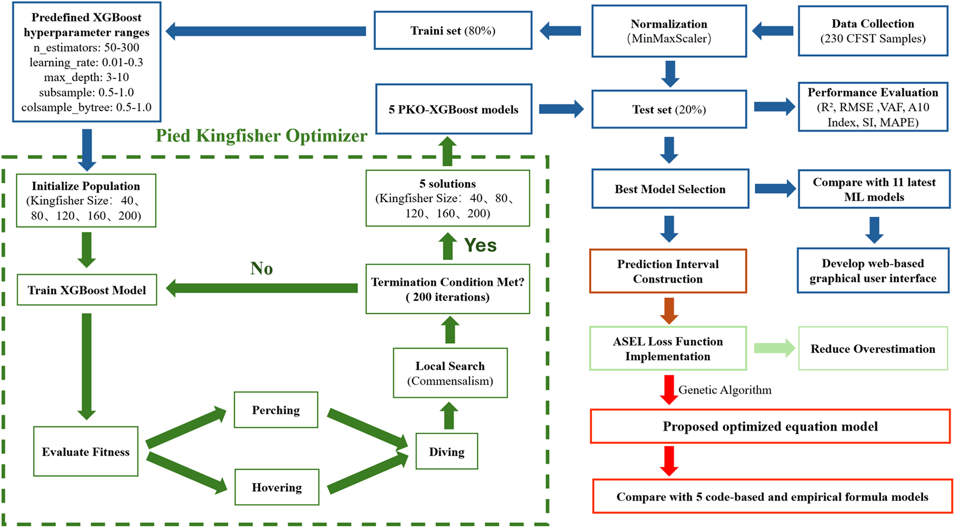
Figure 1: Research workflow for predicting CFST shear strength

2.1 Extreme Gradient Boosting

This study uses the Extreme Gradient Boosting algorithm (XGBoost) for modeling. The gradient boosting method was introduced by Friedman [31], and it is essentially an iterative machine learning algorithm that incrementally builds multiple weak learners, where each learner fits the residuals of the previous learner. XGBoost was introduced by Chen and Guestrin [32], and it incorporates several optimizations on top of the traditional gradient boosting algorithm, including regularization and parallel processing. The key mathematical equations involved in XGBoost are as follows:

2.1.1 Model Prediction Equations

The predicted value of the XGBoost model is composed of the weighted sum of multiple additive functions (decision trees), as shown in Eq. (1):

y^i=∑k=1Kfk(xi)(1)

where y^i is the predicted target of the ith sample, xi is the input variable of the ith sample, and fk is the predicted value for kth decision tree.

2.1.2 Objective Function

The objective function of XGBoost consists of a training loss and a regularization term, and the optimization goal is to minimize this objective function, as shown in Eq. (2):

Obj=∑i=1nl(yi,y^i)+∑k=1KΩ(fk)(2)

where l(yi,y^i) is the loss between the predicted and actual values, and Ω(fk) is the regularization term, used to control model complexity.

Eq. (1) represents that the final prediction result of the model is obtained through the weighted sum of multiple trees, while Eq. (2) represents that the objective function enhances the model’s generalization and stability by minimizing total loss during training. XGBoost achieves efficient gradient boosting and regularization through these two equations, making the model perform excellently in various tasks.

2.2 Pied Kingfisher Optimizer

The Pied Kingfisher Optimizer (PKO) will be applied to optimize the hyperparameters of XGBoost to enhance the model’s performance. The PKO is a metaheuristic optimization algorithm capable of solving complex optimization problems. It is inspired by the unique hunting behavior and symbiotic relationships of the Pied Kingfisher [33]. The core algorithm is divided into two phases, each corresponding to specific behaviors and mathematical models, explained in Sections 2.2.1 and 2.2.2, respectively.

2.2.1 Exploration Phase

This phase mimics the behavior of the Pied Kingfisher searching for prey while perching and hovering, aiming to diversify the search space and avoid premature convergence to local optima. The mathematical model is expressed as shown in Eq. (3):

Xi(t+1)=Xi(t)+a⋅T⋅(Xj(t)−Xi(t))(3)

This equation describes how the search agent updates its position based on its current position and the positions of neighboring individuals during the exploration phase. Here, Xi(t+1) is the new position of the ith individual at the (t + 1)th iteration, Xi(t) is the current position of the ith individual at the tth iteration, a is a random number generated from a normal distribution, and T is a dynamically computed parameter.

2.2.2 Development Phase

The development phase simulates the Pied Kingfisher’s diving behavior to concentrate the search in a specific region. The key equation is expressed as shown in Eqs. (4)–(7):

Xi(t+1)=Xi(t)+HA⋅o⋅a⋅(b−Xbest(t))(4)

where HA is the hunting ability, defined as:

HA=rand⋅PKO Fitness(i)Best Fitness(5)

o is a control parameter, defined as:

o=exp⁡(−tMax Iter)2(6)

Here, a is a random number generated from a normal distribution, and b is a parameter based on the best solution, defined as:

b=Xi(t)+o2⋅randn⋅Xbest(t)(7)

These two equations balance the exploration and development phases, where the parameters o and HA control the search intensity. This ensures that the PKO algorithm can both broadly explore the solution space and focus on potential optimal solutions, effectively avoiding local optimal.

2.3 Genetic Algorithm

This study employs the Genetic Algorithm (GA) to optimize previous work and proposes a design-oriented shear strength equation model with enhanced predictive capabilities. Like the PKO, GA is also a metaheuristic optimization algorithm. Its principle is based on natural selection and genetics, simulating the process of biological evolution to achieve global search and optimization [34]. The optimization begins with an initial population of candidate solutions, encoded as chromosomes. In each generation, the GA iteratively produces better solutions through operations such as selection, crossover, and mutation of chromosomes [35]. Chromosomes are selected based on their fitness, defined as the negative value of the objective function RMSE, where higher fitness indicates that the corresponding parameter combination is closer to optimal. As iterations proceed, those with lower fitness gradually replace chromosomes with higher fitness. The iterative process terminates when significantly high-fitness chromosomes emerge in the population, and the optimal parameter combination is obtained by decoding the final chromosome [36].

In this study, the GA parameters are configured as follows: the population size is set to 100, with a maximum of 1000 iterations. The mutation and crossover probabilities are defined as 0.1 and 0.5, respectively. An elitism ratio of 0.01 is adopted to preserve the best individuals, and 30% of the population is selected as parents in each generation. A uniform crossover scheme is used, and no additional early-stopping criterion is imposed. The fitness function is formulated as the negative RMSE, ensuring that solutions with lower prediction errors are assigned higher fitness values.

2.4 Quantile Regression Model

After training the XGBoost model, a quantile regression model will be used to estimate the prediction interval. Unlike traditional mean regression, quantile regression can estimate lower and upper quantiles to construct the prediction interval [37]. The goal of quantile regression is to find a set of regression coefficients β that minimizes the loss function for a given quantile τ [38]. The mathematical model is expressed as shown in Eq. (8):

β^τ=argminβ∑i=1nρτ(yi−xiTβ)(8)

where arg min denotes the parameter that minimizes the function; yi is the ith true value; xi is the corresponding vector of predictor variables; β is the regression coefficient to be predicted; ρτ is the quantile loss function (check function), which is used to evaluate the residual for each sample point.

The Prediction Interval Coverage Probability (PICP) and the Mean Width of the Prediction Interval (MWPI) are typically calculated to assess the quality of the prediction intervals. These metrics are used to measure the proportion of actual values that fall within the prediction interval and the width of the prediction interval, respectively [39]. The mathematical expressions are expressed as shown in Eqs. (9) and (10):

PICP=1n∑i=1nI(yi∈[y^iL,y^iU])(9)

MWPI=1n∑i=1n(y^iU−y^iL)(10)

where n is the number of samples in the test set, yi is the ith true value, y^iL is the lower bound of the ith prediction interval, y^iU is the upper bound of the ith prediction interval, and I(·) is the indicator function, which takes the value of 1, if yi falls within the interval [y^iL,y^iU], and 0 otherwise.

2.5 Model Evaluation Metrics

To compare the performance of the prediction model with previously developed models, this study uses the coefficient of determination (R2), root mean square error (RMSE) and mean absolute percentage error (MAPE) to evaluate the model. The mathematical expressions for these metrics are expressed as shown in Eqs. (11)–(16):

R2=1−∑i=1n(yi−y^i)2∑i=1n(yi−y¯)2(11)

RMSE=1n∑i=1n(yi−y^i)2(12)

MAPE=1n∑i=1n|yi−y^iyi|×100%(13)

Additionally, three other metrics, VAF, A10 index, and Scattering Index (SI), are used to evaluate the model’s performance further:

VAF=(1−Var(y−y^)Var(y))×100%(14)

A10 index=Number of y^i in [0.9yi,1.1yi]n(15)

SI=RMSEy¯(16)

where yi and y^i represent the experimental and predicted values of Vu, y¯ is the mean of yi, and n is the number of data samples. In an ideal model, the R2, RMSE, VAF, A10-index, and SI values are 1.0, 0.0, 100%, 1.0, and 0.0, respectively.

3  Dataset Description

To develop an accurate XGBoost model for predicting the shear strength (Vu) of CFST, a comprehensive dataset consisting of 230 test results was utilized. These data were sourced from 11 researchers, encompassing a wide range of experimental conditions [8,9,11,14,40–47]. The dataset includes 10 input variables: cross-sectional diameter (D), wall thickness of the steel tube (t), applied axial load (P), axial compressive strength (P0), cross-sectional area of the steel tube (Ast), cross-sectional area of the concrete core (Ac), shear span-to-diameter ratio (a/D), the ratio of applied axial load to axial compressive strength (P/P0), compressive strength of the concrete (fc′), and yield strength of the steel (fy). The output variable is Vu (kN), representing the measured shear strength. The experimental setup and key geometric and material parameters are depicted in Fig. 2. The Vu is calculated as half of the applied lateral load at failure (Pu), following the relationship Vu=Pu2 derived from the static equilibrium condition, where the applied load is equally distributed between the two supports [47].

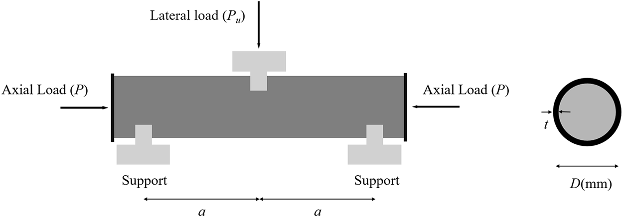
Figure 2: Illustration of CFST members under shear tests

These 230 tests were collected from 11 independent experimental programmes. While the specimens share a common definition of circular CFST members tested in shear, the original studies differ in concrete mixes, steel grades, loading protocols and measurement procedures. To improve consistency, only specimens with complete geometric and material information, shear-dominated failure modes and comparable boundary conditions were retained, and all variables were converted to a common system of units.

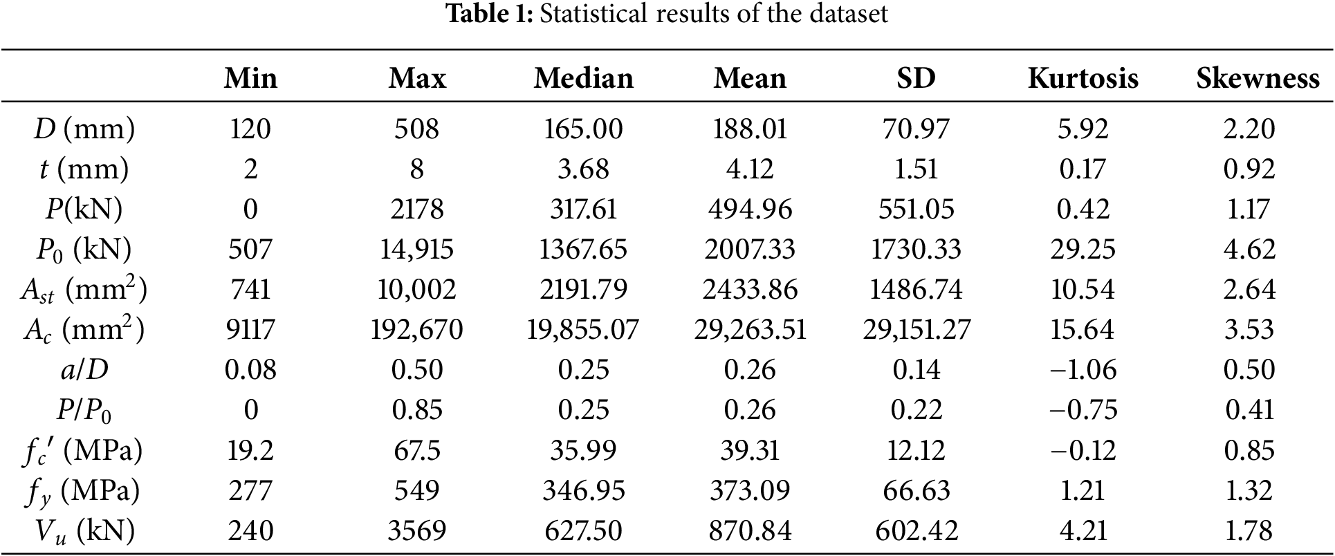
Violin plots and swarm plots are utilized in this study to visually display the distribution of sample sizes and material properties (Fig. 3). The data shows that Ast and Ac exhibit high concentrations with some extreme values. In contrast, the distributions of a/D and P/P0 are relatively uniform but tend to cluster around central values. Additionally, as indicated in Table 1, certain features like P and Vu exhibit large standard deviations, indicating high variability. This variability allows the model to capture a broader spectrum of real-world conditions, making it more robust when applied to unseen data.

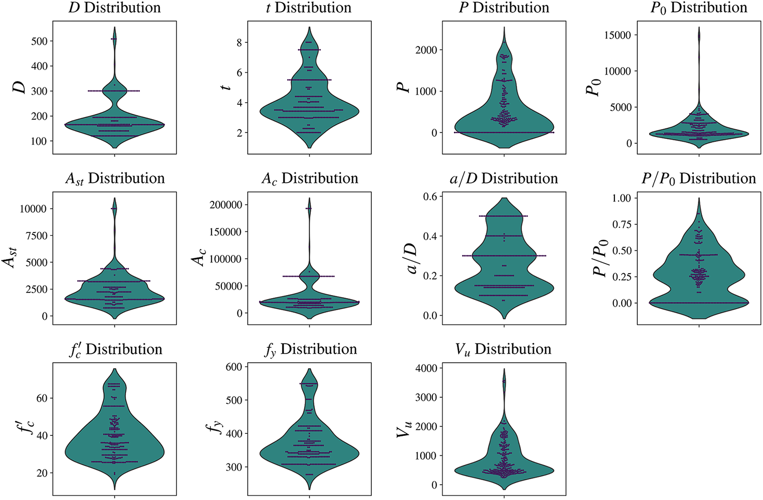
Figure 3: Violin plots with swarm plot overlay showing the distribution of the variables

Moreover, an outlier analysis was carried out on the 230-specimen database. The results showed that 19 specimens (about 8% of the database) were flagged as potentially influential. Only one specimen exhibited a standardized residual slightly greater than 3, while the remaining cases are mainly associated with geometrically or mechanically extreme but physically plausible CFST members (for example, large-diameter, large-section or high axial-load-ratio specimens). Since these specimens do not arise from measurement or recording errors and still lie close to the main prediction trend, no data points were removed and all 230 specimens were retained for model development.

The Pearson correlation matrix presented in Fig. 4 demonstrates that Ast and Ac exhibit the strongest linear correlations with Vu, with coefficients of 0.9 and 0.81, respectively. These are followed by t and P, which show moderate correlations of 0.54 and 0.52. Additionally, variables such as D and P0 display relatively high correlations with Vu (0.84 and 0.87, respectively), while others, such as a/D and P/P0, exhibit weaker correlations. Despite the varying degrees of linear relationships, the interplay among all ten variables will likely involve complex nonlinear interactions that cannot be fully captured by correlation coefficients alone. Thus, leveraging machine learning techniques to establish nonlinear relationships among all ten input variables and Vu is essential to achieve robust and accurate predictions.

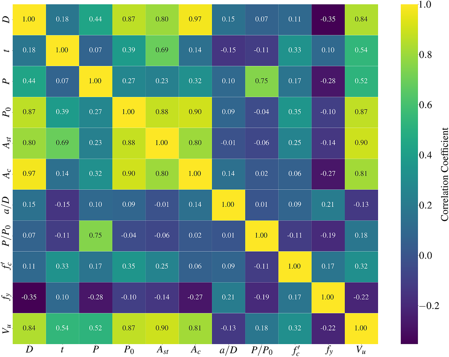
Figure 4: Correlation matrix of the variables

This study randomly divides the data samples into a training set (80%) and a test set (20%). The training set is used to construct the proposed model, named PKO-XGBoost, while the test set is used to evaluate the model’s performance. Since the variables in the dataset have different ranges, variables with larger magnitudes might dominate others. To address this issue, MinMaxScaler is applied to normalize the dataset, scaling the data to the [0, 1] range. The mathematical expression for normalization is expressed as shown in Eq. (17):

Xscaled=X−XminXmax−Xmin(17)

where X is the original data, Xmin and Xmax are the minimum and maximum values of the original data, and Xscaled is the normalized data, which lies within the range [0, 1]. In addition, a 10-fold cross-validation procedure was conducted to further assess the robustness of the model’s performance [28].

4  Results and Discussion

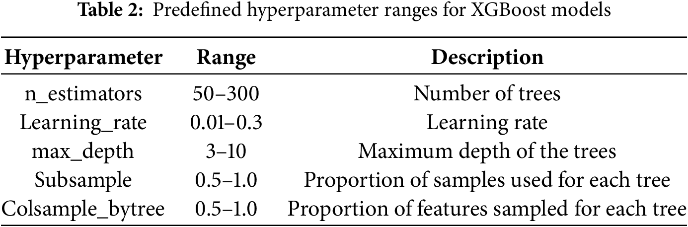
4.1 Determination of Hyperparameters

This section aims to determine the appropriate hyperparameters for the XGBoost model, as shown in Table 2 outlines the predefined hyperparameter ranges. The role of the PKO algorithm is to identify the optimal parameters for the XGBoost model by minimizing the Mean Squared Error (MSE) between the experimental and predicted values of Vu.

The maximum number of iterations for PKO is set to 200, and the Kingfisher population sizes are set to 40, 80, 120, 160, and 200. Therefore, five configurations of XGBoost model hyperparameters will be generated. Fig. 5 shows the evolution of the PKO algorithm with different Kingfisher population sizes. The fitness values (MSE) for all models decrease significantly as the number of iterations increases, indicating continuous improvement in model performance during optimization. The fitness values (MSE) stabilize around 175 iterations, and the model gradually converges to an optimal state. When the Kingfisher population is set to 160 and 200, the fitness values (MSE) decrease rapidly, and the final fitness values are lower, indicating better convergence and improved model performance.

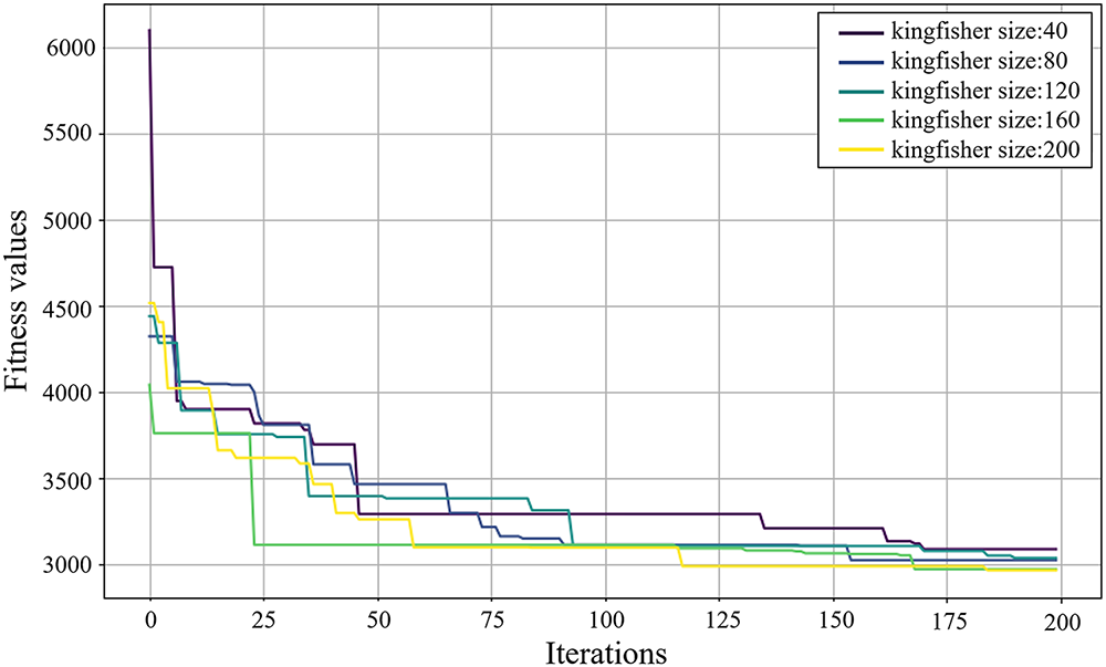
Figure 5: Iteration of the hybrid XGBoost model with different kingfisher sizes

After the computation, the hyperparameter values of the XGBoost model are extracted. Table 3 presents the obtained hyperparameter values for each Kingfisher population size. Although the positions of the four potential solutions for the XGBoost model’s hyperparameters vary, their respective fitness values (RMSE) are similar, indicating that all five XGBoost models demonstrate excellent predictive performance. A further discussion will follow to determine the best model.

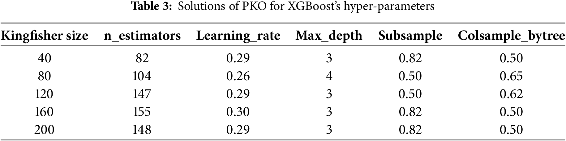
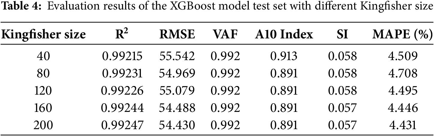
The performance of the five models is presented in Table 4. The VAF values for all models are close to 0.992, indicating similar performance in terms of the ratio of prediction error variance to actual value variance. The model with a Kingfisher population of 200 achieves the highest R2 on the test set, reaching 0.99247, and has the lowest error rate at 4.431%, corresponding to an RMSE of 54.43 kN and a MAPE of 4.431%. Consequently, the hyperparameter configuration of (148, 0.30, 4, 0.82, 0.50) is selected as the optimal setup. In this configuration, 148 decision trees are included, with each tree correcting the predictions of the previous one. The learning rate and maximum depth of the trees are set to 0.3 and 4, respectively. For comparison, when the same hyperparameter ranges and the same number of optimization iterations are used with conventional grid search and random search, the best XGBoost models obtained R2 values of 0.9859 and 0.9857 and RMSE values of 74.5005 and 74.9003 kN, respectively. Thus, under an identical computational budget, PKO reduces the test RMSE by about 27%.

In the 10-fold cross-validation, the proposed PKO-XGBoost model achieved an average R2 of 0.9789 ± 0.0097 and MAPE of 6.39% ± 1.31%. These values provide a more conservative, yet still consistently high, estimate of the model’s predictive capability.

4.2 Performance of the Optimal Model

Fig. 6 compares the predicted and actual Vu for the training and testing sets using the optimal hyperparameter model. The bounded lines at “y = 1.1x” and “y = 0.9x” represent the threshold for a 10% prediction deviation. Additionally, six performance metrics are presented in Fig. 6, collectively confirming the model’s strong predictive ability.

Figure 6: Predicted Vu vs. experimental Vu in ascending form of the training and testing sets (PKO-200-XGBoost)

Fig. 7 displays the errors in the training and testing sets of the PKO-200-XGBoost model. The red line represents the actual data, while the purple (training set) and cyan (testing set) lines represent the model’s predictions. Evidently, the model fits the training data well and performs similarly on the test set. Regarding error distribution, Fig. 8 illustrates the distribution of prediction errors for the PKO-200-XGBoost model, categorized into four ranges: 0%–2%, 2%–5%, 5%–10%, and 10%–100%. More than 60% prediction errors fall within the 0%–2% and 2%–5% ranges, with only 10.9% of the data showing errors exceeding 10%, further demonstrating the model’s high accuracy in predicting Vu.

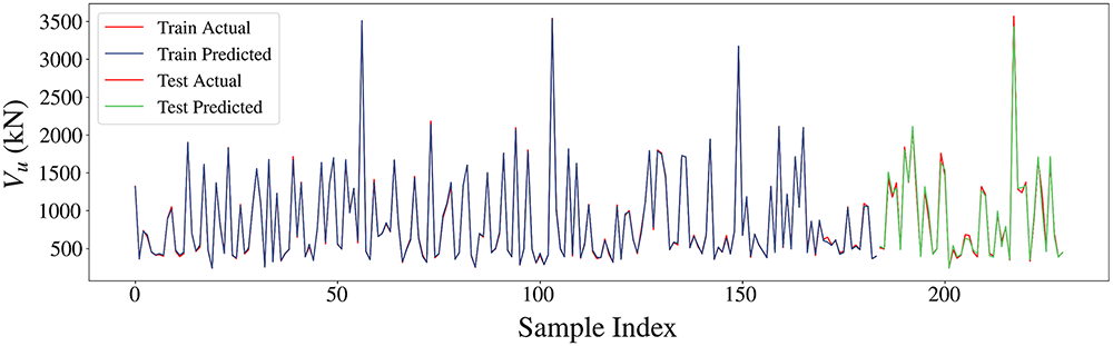
Figure 7: Error distribution of PKO-200-XGBoost on the training set and testing set

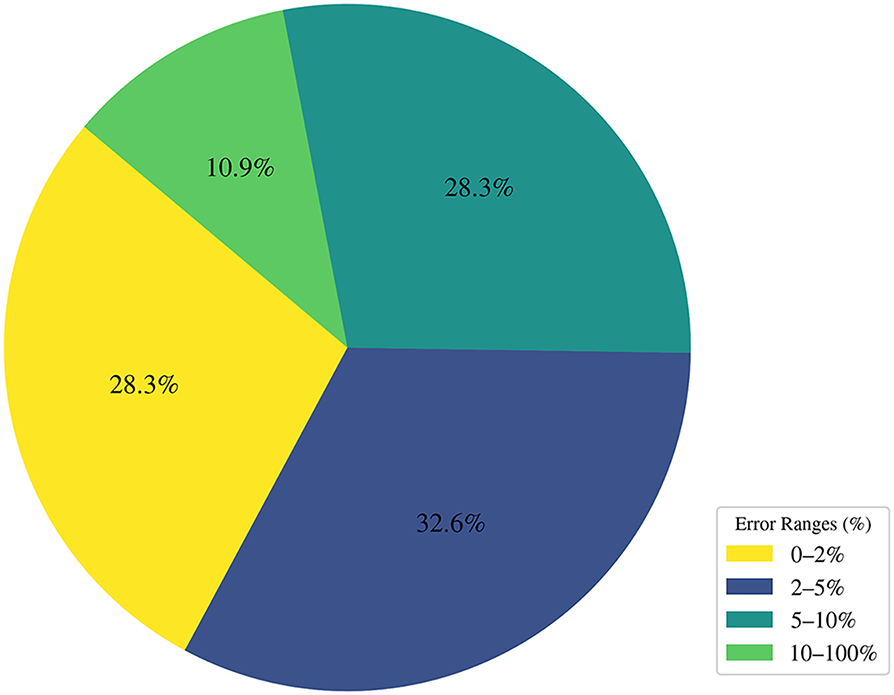
Figure 8: Distribution of residual ranges in the test Set of PKO-200-XGBoost

4.3 Interval Prediction of Vu

The optimal model proposed in the previous section provides accurate prediction results (RMSE of 55.43 and MAPE of 4.431%). However, the model does not offer information about the dispersion around the predicted values. To address this limitation, this study applies the quantile regression technique to derive prediction intervals based on the original model. Specifically, the upper and lower bounds are estimated using the XGBoost model with quantile regression parameters τ = 0.025 and τ = 0.975, mathematically expressed as Q0.025(x) and Q0.975(x). Fig. 9 presents the prediction intervals for the test set, which includes 46 samples. The red dots represent the predicted values for each sample, while the teal shading represents the prediction intervals, with the bounds calculated by the quantile regression model. During the testing phase, the PICP and MWPI were 82.61% and 723.66 kN.

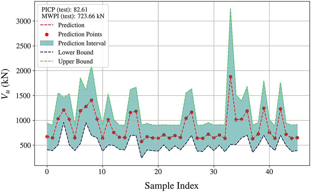
Figure 9: Prediction intervals constructed by XGBoost and quantile regression method

Although the intervals remain of moderate width, the empirical coverage is lower than the nominal confidence level of 95%, indicating a certain degree of undercoverage. This reflects the trade-off between coverage and interval width, and adopting more extreme quantiles could increase PICP but would also produce much wider and less practical intervals. Even with this limitation, the XGBoost model with quantile regression provides reasonably accurate interval estimates and controlled uncertainty, thereby making the Vu predictions for CFST more reliable and informative for design.

4.4 The Model with the Asymmetric Squared Error Loss

In engineering applications, if the predicted value exceeds the actual value, leading to negative residuals, the target variable may be overestimated, posing safety concerns. In contrast, underestimation provides a more conservative approach, reducing potential risks. Therefore, avoiding overestimation is necessary to ensure the model’s applicability in engineering practice.

In the training of the XGBoost model, the standard Squared Error Loss (SEL) is widely used. SEL is a common regression loss function that measures the error between predicted and actual values. Since SEL is symmetric, XGBoost treats positive and negative residuals equally during training. Mathematically, the residual is defined as:

ε=t−y(18)

where t represents the actual value of Vu, and y is the predicted value. When the actual value is less than predicted, the residual is negative, and vice versa. Theoretically, for XGBoost models trained using SEL, the proportion of positive and negative residuals should be relatively balanced, meaning that overestimation and underestimation should occur with equal frequency.

Fig. 10 shows the residual distribution of the model trained with SEL. Most residuals are concentrated between −50 and 50, indicating that the model’s prediction error is small, and the residuals approximately follow a normal distribution. Statistical data show that the mean residual is 0.05, the standard deviation is 28.40, and the skewness is 0.11, indicating near-symmetry. Fig. 11 provides further details on the residuals, where the mean of the positive residuals is 19.78, slightly higher than the mean of the negative residuals, which is 16.24. These data suggest slight differences between positive and negative residuals, but the overall distribution is symmetrical.

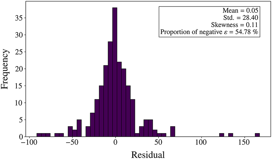
Figure 10: Distribution of residuals obtained from the model using SEL

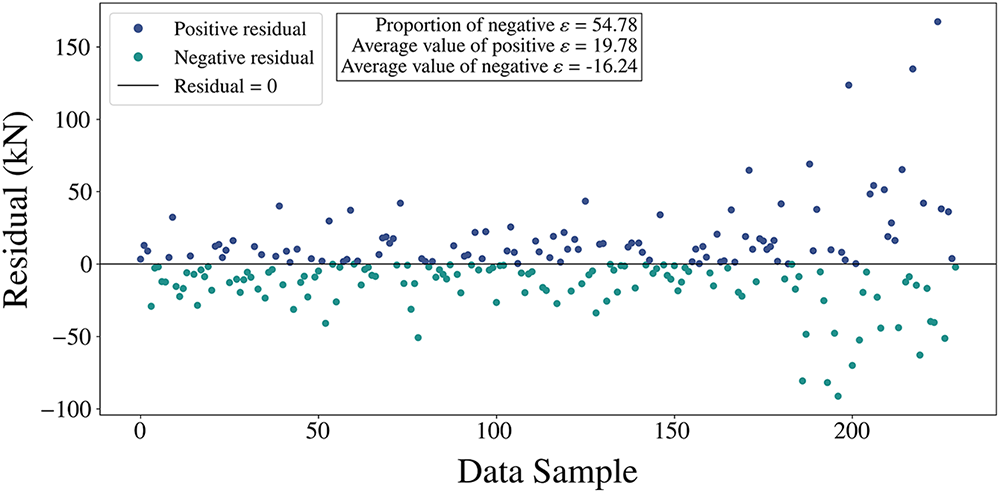
Figure 11: Magnitude of positive and negative residuals obtained from the model using SEL

This study employs Asymmetric Squared Error Loss (ASEL) to train the PKO-XGBoost model to reduce the probability of overestimation in the model. The ASEL function for each sample is expressed as shown in Eq. (19):

Li={ρ(ti−yi)2if yi>ti(ti−yi)2if yi≤ti(19)

where the parameter ρ controls the degree of asymmetry in the loss function, as the value of ρ increases, the penalty for overestimation becomes more severe. To implement the ASEL function in XGBoost, this study customizes the Gradient and Hessian of the loss function within the model and modifies them as follows Eqs. (20) and (21):

Gradient:

Li′={2ρ(ti−yi),if yi>ti2(ti−yi),if yi≤ti(20)

Hessian:

Li′′={2ρ,if yi>ti2,if yi≤ti(21)

This study tested different values of ρ to train the PKO-XGBoost model. The training results for various ρ values are shown in Fig. 12. As ρ increases from 10 to 50, the proportion of positive residuals gradually increases, indicating a reduction in the proportion of overestimations. When ρ = 50, the proportion of positive residuals reaches 72%.

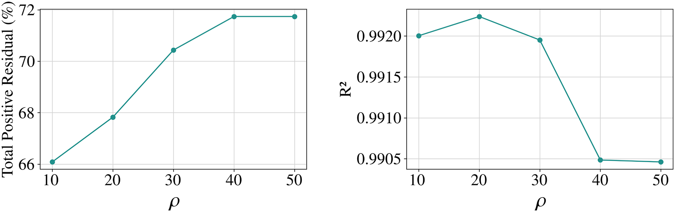
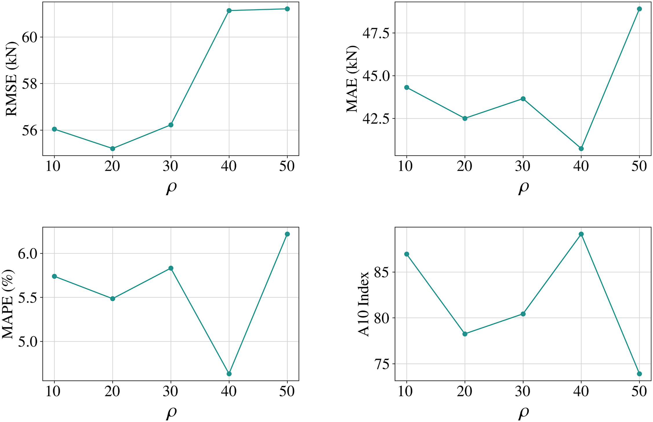
Figure 12: Line graph of the change in performance of the PKO-XGBoost model for different values of ρ

However, the model’s predictive performance declines as the overestimation rate decreases. For instance, at ρ = 50, the model’s MAPE is the highest, indicating the most significant error rate. Therefore, evaluating the five models’ performance from multiple dimensions is essential. From the Fig. 12, when ρ = 40, the model achieves near-maximum positive residuals (72%) and performs well on several metrics, including R2 (0.9905), RMSE (61.13), MAE (40.74), MAPE (4.63), and the A10 index (89.13). Consequently, ρ = 40 is the optimal parameter for training the ASEL-PKO-XGBoost model.

The ASEL-PKO-XGBoost model with ρ = 40 demonstrates significant improvement in residual characteristics. First, the mean residual increased from 0.05 to 17.44 (as shown in Fig. 13), indicating a notable shift in the residual distribution. Specifically, most residuals are now skewed to the right of the horizontal axis, with a significant reduction in overestimation, as the proportion of overestimations decreased from 54.75% to 28.26%. This change suggests that the model’s predictions for the target values are more accurate and less biased. Additionally, as shown in Fig. 14, many predicted points are concentrated in the upper half of the plot, further reflecting the reduction in overestimation.

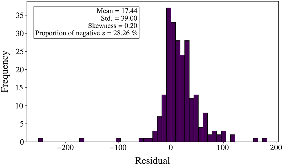
Figure 13: Distribution of residuals obtained from the model using ASEL

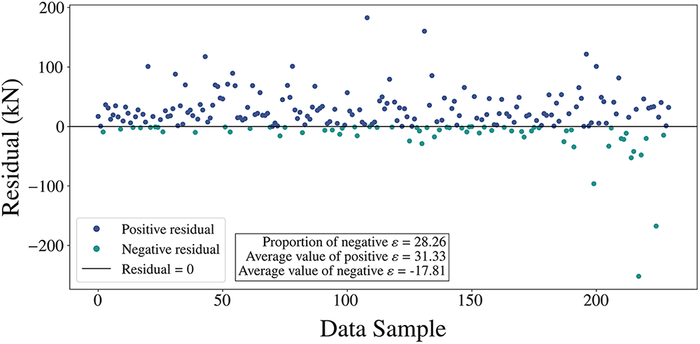
Figure 14: Magnitude of positive and negative residuals obtained from the model using ASEL

Regarding residual polarity, the average positive residual is 31.33 kN, while the average negative residual is −17.81 kN. This indicates that while the model exhibits a more significant bias for underestimation, the frequency and magnitude of overestimations are smaller. This characteristic of the residual distribution reflects the stability of the predicted results.

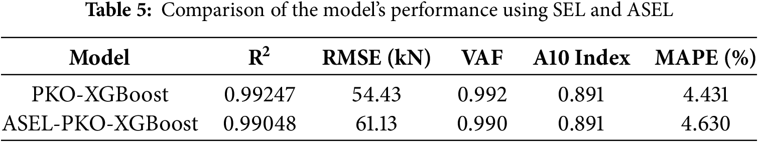
Fig. 15 presents the prediction results of the PKO-XGBoost model trained with ASEL (ρ = 40). The model achieved an RMSE of 61.13 and a MAPE of 4.632%, demonstrating strong predictive performance. Although the introduction of ASEL slightly reduced the model’s overall performance, it remains excellent (R2 > 0.99). Table 5 provides a detailed comparison of the performance of models trained with two different loss functions (SEL and ASEL). The differences between the two models across the performance metrics (R2, RMSE, VAF, A10 index, and MAPE) are minimal. Both models achieved an A10 index of 0.891, indicating that 89.1% of the predicted values have a relative error within 10% of the actual values. However, the ASEL-PKO-XGBoost model significantly reduced the overestimation of Vu compared to the PKO-XGBoost model, making it a more reliable option.

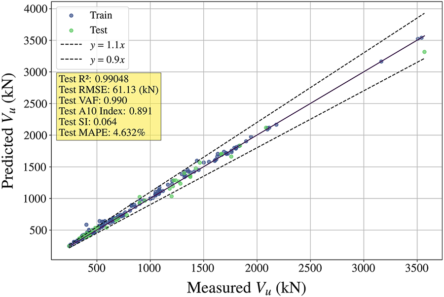
Figure 15: Prediction outcomes of PKO-XGBoost trained with ASEL

Although the ASEL-based model introduces a slight overall underestimation, its role is not to replace the partial safety factors prescribed in design codes. In practice, the ASEL-based predictions should still be combined with the usual safety factors. This “ASEL + safety factor” combination is more conservative than applying the safety factors to a symmetric-error model alone.

Statistical tests were applied to the residuals of both the PKO-XGBoost and ASEL-PKO-XGBoost. For the PKO-XGBoost, the Shapiro–Wilk test yielded a statistic of 0.9458 with p = 0.0322, and the Breusch–Pagan test (LM = 10.38, p = 0.0013; F = 12.82, p = 0.0009) indicated non-constant variance across the range of predicted Vu. For the ASEL-PKO-XGBoost, the Shapiro–Wilk statistic further decreased to 0.8442 with p < 0.0001, and the Breusch–Pagan test (LM = 16.62, p < 0.0001; F = 24.88, p < 0.0001) confirmed a more pronounced deviation from normality and homoscedasticity. These imperfections in the error structure are considered reasonable for an aggregated multi-source experimental database

4.5 Comparison with Latest Machine Learning Models

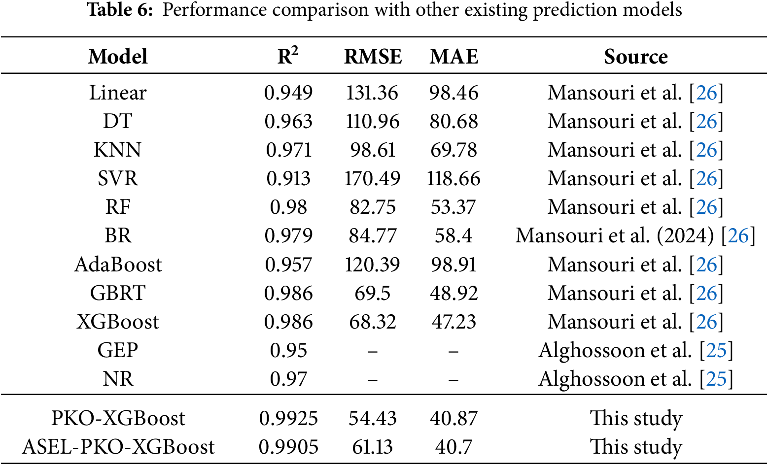
In order to validate the superiority of the PKO-XGBoost and ASEL-PKO-XGBoost models, the proposed model is compared with 11 of the latest prediction models presented by other researchers in the field [25,26]. Table 6 shows the performance comparison of different machine learning models in predicting Vu. The models proposed in this study achieve competitive accuracy, with higher R2 and lower RMSE and MAE than the benchmark models. Due to differences in datasets and train–test splits among the published studies, this comparison should be interpreted as a reference rather than a fully controlled benchmark.

4.6 Proposed Optimized Vu Equation

Although PKO-XGBoost and ASEL-PKO-XGBoost achieve high accuracy in predicting CFST shear strength (Vu), their lack of interpretability remains a limitation. An equation-based model optimized by Genetic Algorithm (GA) is proposed to address this limitation, enabling engineers to quickly and accurately estimate Vu. This equation model can be used in conjunction with machine learning models, allowing engineers to leverage the simplicity of equations for preliminary designs while benefiting from the predictive power of XGBoost models for detailed analyses.

4.6.1 Construction of Vu Equation Model

In this field, the equation model proposed by Roeder is considered superior to standards such as Eurocode and AISC [26,27,48]. This model introduces γ as a coefficient to account for the effect of the axial load ratio P/P0 on shear strength. The expression for γ is:

γ=5⋅(1+5⋅PP0)(22)

After simplification, the model proposed by Roeder can be expressed as:

Vn=0.6⋅fy⋅As+0.415⋅fc′⋅Ac+2.075⋅PP0⋅fc′⋅Ac,for γ≤10(23a)

Vn=0.6⋅fy⋅As+0.83⋅fc′⋅Ac,for γ>10(23b)

By introducing the coefficients C1, C2, C3, C4 and C5, the model to be optimized is expressed as:

Vn=C1⋅fy⋅As+C2⋅fc′⋅Ac+C3⋅PP0⋅fc′⋅Ac,for γ≤10(24a)

Vn=C4⋅fy⋅As+C5⋅fc′⋅Ac,for γ>10(24b)

The coefficients C1–C5 act as weighting factors for the main mechanical contributions to the shear capacity. Coefficients C1 and C4 scale the term fyAs and therefore quantify the direct contribution of the steel tube to Vn in the γ ≤ 10 and γ > 10 egimes, respectively. Coefficients C2 and C5 weight the term fc′Ac, representing the contribution of the confined concrete core, which increases with both concrete strength and core area. Coefficient C3 multiplies the interaction term (P/P0)fc′Ac, capturing the influence of the axial load ratio on mobilising confinement and shear transfer in the concrete.

4.6.2 Optimization Proposed Equation Model

The Genetic Algorithm (GA) determines the equation’s optimal values for coefficients C1 to C5. The ranges for the coefficients are defined as C1 [0, 2], C2 ∈ [0, 2], C3 ∈ [0, 3], C4 ∈ [0, 2] and C5 ∈ [0, 3]. Eighty percent of the database is used for coefficient optimization, with the remaining 20% reserved to validate the optimized model’s predictive performance on test data. The optimal coefficient combination obtained is: C1 = 0.602; C2 = 0.898; C3 = 0.008; C4 = 0.664; C5 = 2.153. Substituting these values into the equation yields:

 Vn=0.602⋅fy⋅As+0.898⋅fc′⋅Ac+0.008⋅PP0⋅fc′⋅Ac,for γ≤10(25a)

Vn=0.664⋅fy⋅As+2.153⋅fc′⋅Ac,for γ>10(25b)

For the case of γ≤10, the RMSE and R2 of the test set are 116.96 and 0.972, respectively. However, when γ>10, the RMSE and R2 are 270.02 and 0.71, respectively. This indicates that the optimized equation fails to adequately capture the variables’ influence on shear strength γ>10.

To improve the model’s predictive performance, a hybrid approach is adopted by incorporating the shear strength equation proposed by Alghossoon et al. [25] specifically for γ>10. Consequently, the improved equation is named the Hybrid GA-Optimized Shear Strength Model (HSM), and it is expressed as shown in Eqs. (26a) and (26b):

Vn=0.602⋅fy⋅As+0.898⋅fc′⋅Ac+0.008⋅PP0⋅fc′⋅Ac,for γ≤10(26a)

Vn=Acfc′(4.0PPno+0.63)+Asfy(1−aD)−110,for γ>10(26b)

The HSM, optimized through GA, has significantly enhanced predictive accuracy by reintegrating key influencing factors, including the contributions of steel and concrete, the correction effect of P/P0 on structural performance, and the weakening effect of a/D on shear capacity.

4.6.3 Comparison with Existing Equation Models

In this section, the accuracy of the HSM model is evaluated by comparing it with five code-based and empirical equation models: Eurocode 4 [27] (p. 4), AISC [48], Xiao’s equation [46], Roeder’s equation [49], Abdullah’s equation [25].

As shown in Fig. 16, the proposed HSM demonstrates superior fitting capability (R2 = 0.934) and error control (RMSE = 153.852 kN, MAE = 116.023 kN) compared to other equations, with Abdullah’s equation ranking second. In contrast, Eurocode 4 and AISC exhibit significant underestimation due to overly simplistic assumptions, rendering them almost incapable of accurately predicting Vu. Roeder’s and Xiao’s equations provide relatively accurate predictions within specific ranges but show significantly higher overall errors than HSM.

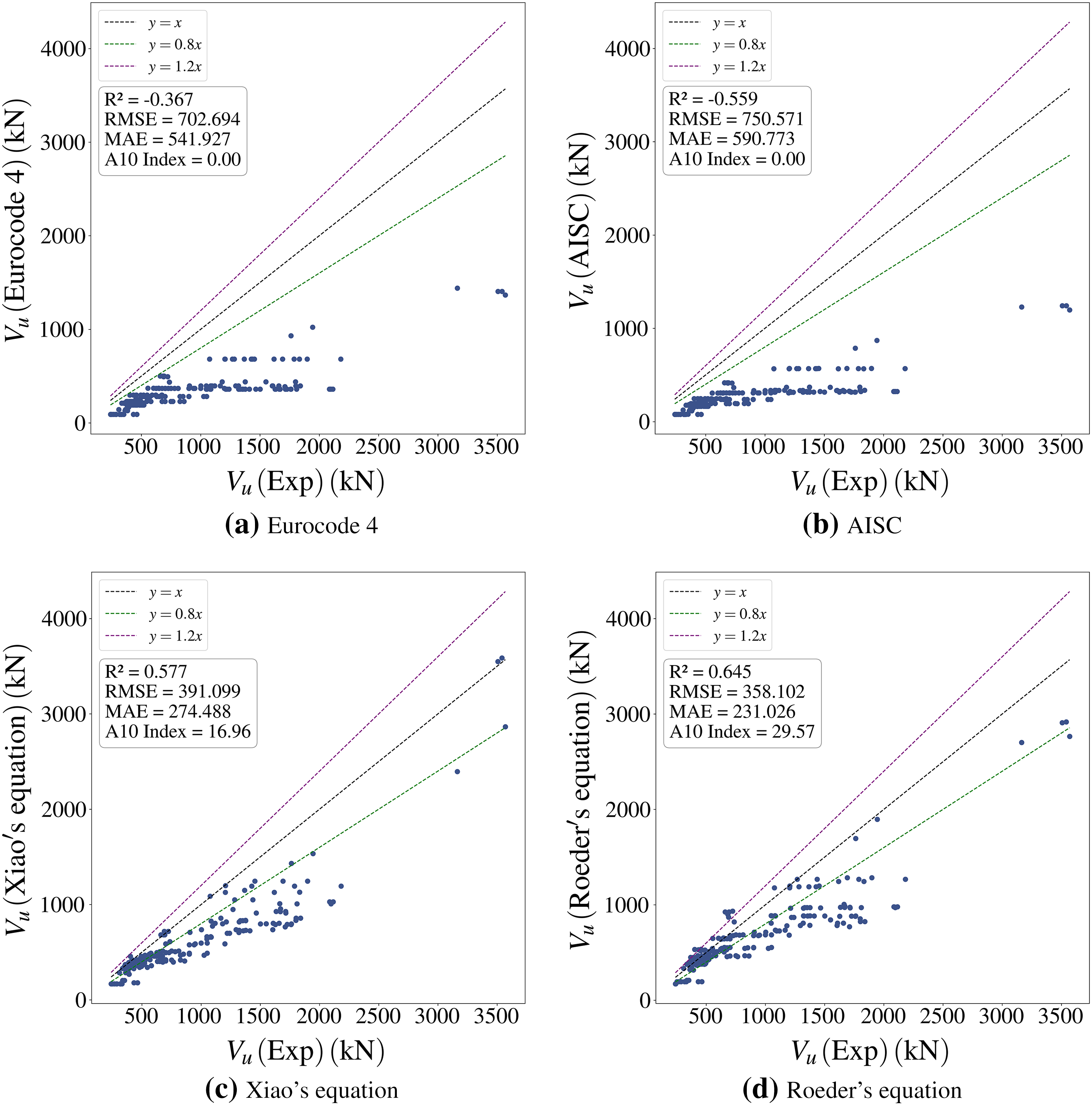
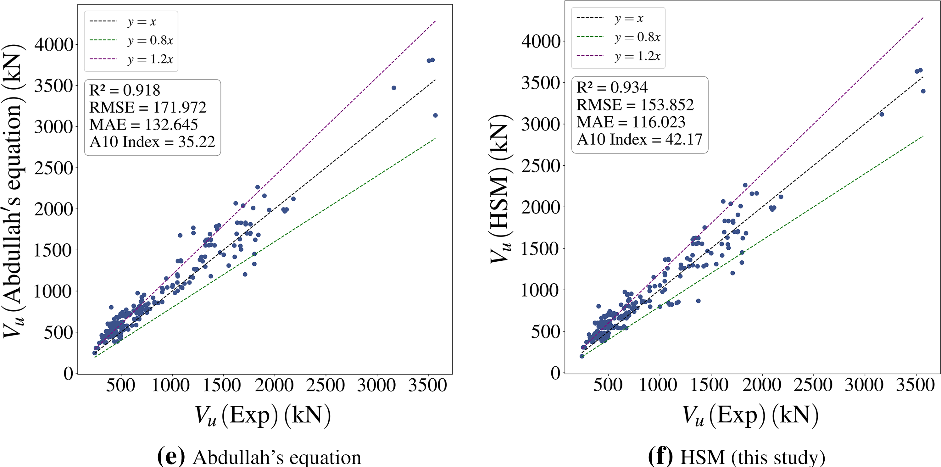
Figure 16: Comparison of Vu prediction performance using different code-based and empirical models

4.7 Graphical User Interface (GUI)

To enhance the accessibility and usability of the proposed PKO-XGBoost and ASEL-PKO-XGBoost models, a web-based Graphical User Interface (GUI) was developed (Fig. 17). The GUI enables users to input key design parameters and obtain accurate real-time predictions of Vu for CFST (R2 > 0.99). While the PKO-XGBoost model (Fig. 17a) provides standard point predictions together with the associated prediction intervals obtained from the quantile-regression model, the ASEL-PKO-XGBoost model (Fig. 17b) addresses the risk of overestimation by offering conservative (underestimated) point predictions, ensuring enhanced safety margins in structural design. All input (D, t, P, P0, Ast, Ac, a/D, P/P0, fc′ and fy) are constrained to the calibrated ranges of the database (120–508, 2–8 mm, 0–2178, 507–14,915 kN, 741–10,002, 9117– 192,670 mm2, 0.08–0.50, 0–0.85, 19.2–67.5 and 277–549 MPa, respectively) in order to avoid obviously unrealistic combinations. When an input lies outside these ranges, the models can still generate predictions. However, such extrapolative results may be unreliable and should be interpreted with caution.

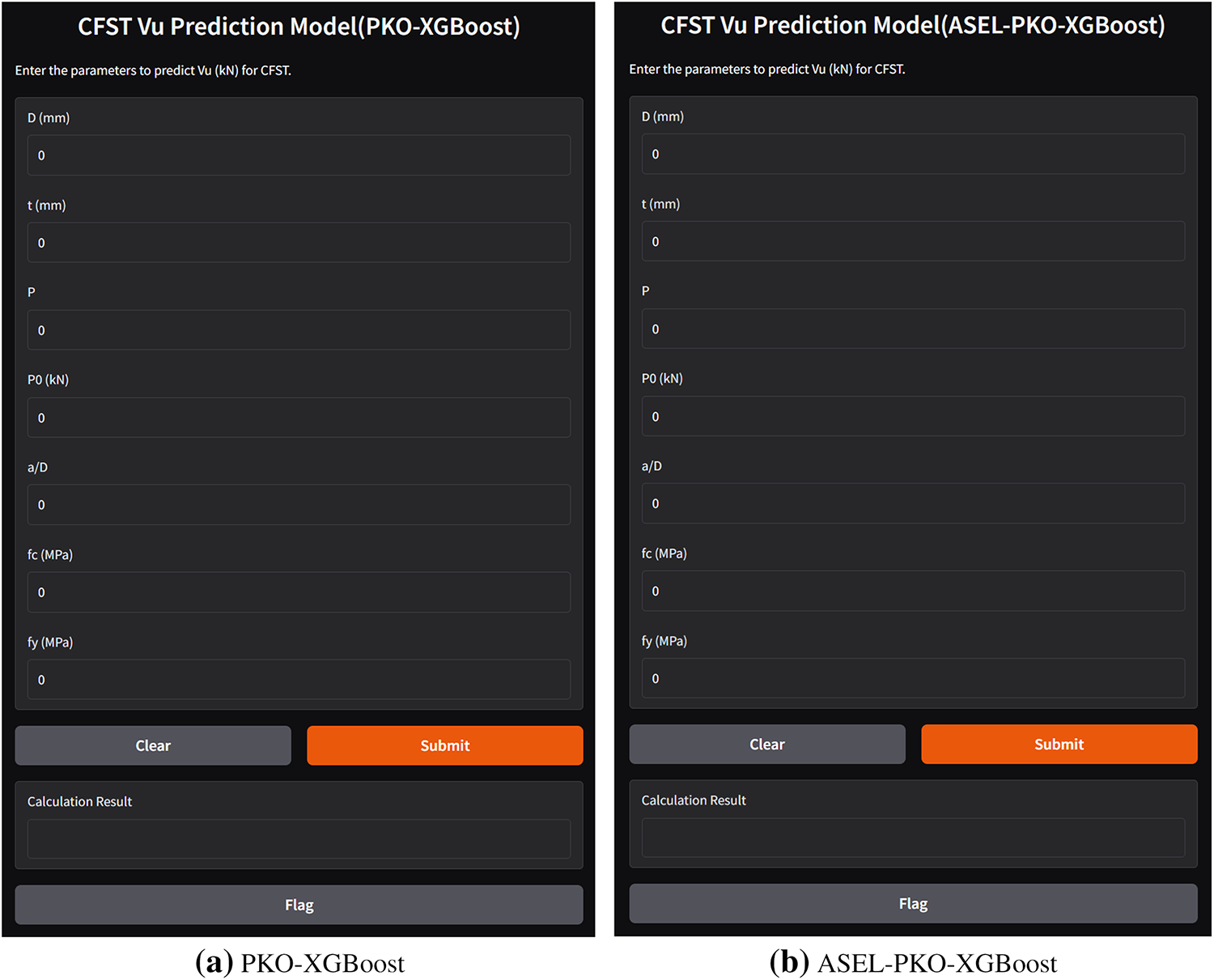
Figure 17: GUI for predicting Vu of CFST

5  Conclusions

This study employs metaheuristic optimization techniques, including the Pied Kingfisher Optimizer (PKO) and Genetic Algorithm (GA), combined XGBoost, to accurately predict the shear strength (Vu) of CFST. The proposed approach demonstrates superior predictive performance compared to traditional equations and recent machine learning models, while also addressing limitations in predictive uncertainty by introducing quantile regression. A design-oriented equation model and a user-friendly graphical user interface (GUI) are also developed for practical applications. The main findings of this study are summarized as follows:

1.    The PKO-XGBoost model achieved an R2 of 0.9925, RMSE of 54.43 kN and MAPE of 4.431%, surpassing the 11 latest machine learning models in the same field.

2.    Quantile regression provided reliable prediction intervals (PICP = 82.61%, MWPI = 723.66 kN).

3.    The ASEL-PKO-XGBoost model reduced the overestimation rate from 50% to 28.26% while maintaining strong performance (R2 = 0.9905).

4.    The proposed equation model (HSM) was developed using GA, achieving better prediction accuracy than five existing equation models based on codes and empirical data (R2 = 0.934).

The quantile-regression-based prediction intervals currently exhibit undercoverage with respect to the nominal confidence level, and no systematic comparison with alternative uncertainty-quantification techniques has yet been performed. Future work will therefore focus on improving the calibration of the prediction intervals and benchmarking the present approach against other uncertainty quantification methods to enhance the reliability of risk-informed CFST design.

Although the proposed Hybrid GA-Optimized Shear Strength Model (HSM) achieves the highest overall predictive accuracy among the existing equation models, it is constructed by switching between two empirical equations at γ = 10. As a result, the transitional continuity and mechanical consistency of this piecewise formulation have not been rigorously established. Future work will therefore focus on developing a more unified, mechanics-informed expression for Vu. In addition, all models, including the HSM, were developed and evaluated on the same 230-specimen database, and their performance on completely independent datasets with different geometries and material grades remains to be verified in future work.

Moreover, the present study does not derive or calibrate a fully mechanics-based shear model, which is recognized as a limitation and will be addressed in future work by systematically linking data-driven models with rigorously formulated mechanical theories.

Acknowledgement: Not applicable.

Funding Statement: This research was funded by United Arab Emirates University (UAEU) under the UAEU-AUA grant number G00004577 (12N145), with the corresponding grant at Universiti Malaya (UM) under grant number IF019-2024.

Author Contributions: The authors confirm contribution to the paper as follows: Conceptualization, Soon Poh Yap and Shengkang Zhang; methodology, Shengkang Zhang; software, Shengkang Zhang and Haoyun Fan; validation, Shengkang Zhang and Shiyuan Li; formal analysis, Shengkang Zhang; investigation, Shengkang Zhang; resources, Haoyun Fan, Shiyuan Li, and Yong Jin; data curation, Shengkang Zhang; writing—original draft preparation, Shengkang Zhang; writing—review and editing, Soon Poh Yap, Yong Jin, Ahmed El-Shafie and Amr El-Dieb; visualization, Shengkang Zhang; supervision, Soon Poh Yap, Ahmed El-Shafie and Zainah Ibrahim; project administration, Zainah Ibrahim; funding acquisition, Yong Jin, Zainah Ibrahim and Amr El-Dieb. All authors reviewed the results and approved the final version of the manuscript.

Availability of Data and Materials: The data that support the findings of this study are available from the corresponding author upon reasonable request. The code implementing the PKO–XGBoost model and the associated training and evaluation procedures is openly available in the GitHub repository “CFST-Vu-Shear-Strength” at: https://github.com/zhangshengkang/CFST-Vu-Shear-Strength (accessed on 12 December 2025).

Ethics Approval: Not applicable.

Conflicts of Interest: The authors declare no conflicts of interest to report regarding the present study.

References

1. Han LH. Flexural behaviour of concrete-filled steel tube. J Constr Steel Res. 2004;60(2):313–37. [Google Scholar]

2. Luo K, Pi Y, Gao W, Bradford M. Creep of concrete core and time-dependent non-linear behaviour and buckling of shallow concrete-filled steel tubular arches. Comput Model Eng Sci. 2013;95(1):31–58. doi:10.1201/b13139-96. [Google Scholar] [CrossRef]

3. Aguirre DA, Kowalsky MJ, Nau JM, Gabr M, Lucier G. Seismic performance of reinforced concrete filled steel tube drilled shafts with inground plastic hinges. Eng Struct. 2018;165:106–19. doi:10.1016/j.engstruct.2018.03.034. [Google Scholar] [CrossRef]

4. Kenarkoohi M, Hassan M. Review of accelerated construction of bridge piers—methods and performance. Adv Bridge Eng. 2024;5(1):3. doi:10.1186/s43251-024-00116-6. [Google Scholar] [CrossRef]

5. Pi YL, Bradford M. Long-term analyses of concrete-filled steel tubular arches accounting for Interval uncertainty. Comput Model Eng Sci. 2014;99(3):233–53. [Google Scholar]

6. Roeder CW, Stephens MT, Lehman DE. Concrete filled steel tubes for bridge pier and foundation construction. Int J Steel Struct. 2018;18(1):39–49. doi:10.1007/s13296-018-0304-7. [Google Scholar] [CrossRef]

7. Li S, Han LH, Wang FC, Hou CC. Seismic behavior of fire-exposed concrete-filled steel tubular (CFST) columns. Eng Struct. 2020;224:111085. doi:10.1016/j.engstruct.2020.111085. [Google Scholar] [CrossRef]

8. Kenarangi H, Bruneau M. Investigation of cyclic-shear behavior of circular-reinforced concrete-filled Steel tubes. J Struct Eng. 2020;146(5):04020057. doi:10.1061/(asce)st.1943-541x.0002598. [Google Scholar] [CrossRef]

9. Yang ZC, Han LH, Hou C. Performance of recycled aggregate concrete-filled steel tubular columns under combined compression and shear load. Eng Struct. 2022;253:113771. doi:10.1016/j.engstruct.2021.113771. [Google Scholar] [CrossRef]

10. Wu B, Xu Z, Liu Q, Liu W. Test of the shear behavior of thin-wall steel tubular columns filled with demolished concrete segments/lumps. Anal Chem. 2010;43:12–21. (In Chinese). doi:10.4028/www.scientific.net/kem.517.958. [Google Scholar] [CrossRef]

11. Qian J, Cui Y, Fang X. Shear strength tests of concrete filled steel tube columns. China Civ Eng J. 2007;40(5):1–9. (In Chinese). [Google Scholar]

12. Han LH, Tao Z, Yao GH. Behaviour of concrete-filled steel tubular members subjected to shear and constant axial compression. Thin-Walled Struct. 2008;46(7):765–80. doi:10.1016/j.tws.2008.01.026. [Google Scholar] [CrossRef]

13. Jung EB, Lee SH, Yoo JH, Roeder C, Lehman D. Shear behavior of large-diameter concrete filled tube (CFT). Int J Steel Struct. 2017;17(4):1651–65. doi:10.1007/s13296-017-1229-2. [Google Scholar] [CrossRef]

14. Xu C, Haixiao L, Chengkui H. Experimental study on shear resistance of self-stressing concrete filled circular steel tubes. J Constr Steel Res. 2009;65(4):801–7. doi:10.1016/j.jcsr.2008.12.004. [Google Scholar] [CrossRef]

15. Yu Y, Al-Damad IMA, Foster S, Nezhad AA, Hajimohammadi A. Compressive strength prediction of fly ash/slag-based geopolymer concrete using EBA-optimised chemistry-informed interpretable deep learning model. Dev Built Environ. 2025;23:100736. doi:10.1016/j.dibe.2025.100736. [Google Scholar] [CrossRef]

16. Yu Y, Jayathilakage R, Liu Y, Hajimohammadi A. Intelligent compressive strength prediction of sustainable rubberised concrete using an optimised interpretable deep CNN-LSTM model with attention mechanism. Appl Soft Comput. 2025;185:113993. doi:10.1016/j.asoc.2025.113993. [Google Scholar] [CrossRef]

17. Hou C, Zhou XG. Strength prediction of circular CFST columns through advanced machine learning methods. J Build Eng. 2022;51:104289. doi:10.1016/j.jobe.2022.104289. [Google Scholar] [CrossRef]

18. Le TT. Practical machine learning-based prediction model for axial capacity of square CFST columns. Mech Adv Mater Struct. 2022;29(12):1782–97. doi:10.1080/15376494.2020.1839608. [Google Scholar] [CrossRef]

19. Vu QV, Truong VH, Thai HT. Machine learning-based prediction of CFST columns using gradient tree boosting algorithm. Compos Struct. 2021;259:113505. doi:10.1016/j.compstruct.2020.113505. [Google Scholar] [CrossRef]

20. Zhou XG, Hou C, Peng J, Yao GH, Fang Z. Structural mechanism-based intelligent capacity prediction methods for concrete-encased CFST columns. J Constr Steel Res. 2023;202:107769. doi:10.1016/j.jcsr.2022.107769. [Google Scholar] [CrossRef]

21. Faridmehr I, Nehdi ML. Predicting axial load capacity of CFST columns using machine learning. Struct Concr. 2022;23(3):1642–58. doi:10.1002/suco.202100641. [Google Scholar] [CrossRef]

22. Hou C, Zhou XG, Shen L. Intelligent prediction methods for N-M interaction of CFST under eccentric compression. Arch Civ Mech Eng. 2023;23(3):197. doi:10.1007/s43452-023-00734-3. [Google Scholar] [CrossRef]

23. Rong Y, Yang L, Xie W, Jiang L. Bearing capacity of rectangular concrete-filled steel tube (CFST) and dumbbell shaped CFST under axial compression, eccentric compression, and pure bending stress states. Zenodo. 2023. doi:10.5061/dryad.905qfttrx. [Google Scholar] [CrossRef]

24. Liu J, Li S, Guo J, Xue S, Chen S, Wang L, et al. Machine learning (ML) based models for predicting the ultimate bending moment resistance of high strength steel welded I-section beam under bending. Thin-Walled Struct. 2023;191:111051. doi:10.1016/j.tws.2023.111051. [Google Scholar] [CrossRef]

25. Alghossoon A, Tarawneh A, Almasabha G, Murad Y, Saleh E, Yahia HA, et al. Shear strength of circular concrete-filled tube (CCFT) members using human-guided artificial intelligence approach. Eng Struct. 2023;282:115820. doi:10.1016/j.engstruct.2023.115820. [Google Scholar] [CrossRef]

26. Mansouri A, Mansouri M, Mangalathu S. Interpretable machine learning model for shear strength estimation of circular concrete-filled steel tubes. Struct Des Tall Spec Build. 2024;33(12):e2111. doi:10.1002/tal.2111. [Google Scholar] [CrossRef]

27. Johnson RP, Anderson D. Designers’ guide to EN 1994-1-1: eurocode 4: design of composite steel and concrete structures. In: General rules and rules for buildings. London, UK: Thomas Telford; 2004. 272 p. [Google Scholar]

28. La H, Nguyen T, Pham TA. A novel hybrid metaheuristic-Bayesian machine learning model for accu-rate load-displacement prediction of pile foundations. Eng Struct. 2025;343:121131. doi:10.1016/j.engstruct.2025.121131. [Google Scholar] [CrossRef]

29. Ke Y, Zhang SS, Jedrzejko MJ, Lin G, Li WG, Nie XF. Strength models of near-surface mounted (NSM) fibre-reinforced polymer (FRP) shear-strengthened RC beams based on machine learning approaches. Compos Struct. 2024;337:118045. doi:10.1016/j.compstruct.2024.118045. [Google Scholar] [CrossRef]

30. Hoang ND, Tran VD, Tran XL. Predicting compressive strength of high-performance concrete using hybridization of nature-inspired metaheuristic and gradient boosting machine. Mathematics. 2024;12(8):1267. doi:10.3390/math12081267. [Google Scholar] [CrossRef]

31. Friedman JH. Greedy function approximation: a gradient boosting machine. Ann Stat. 2001;29(5):1189–232. doi:10.1214/aos/1013203451. [Google Scholar] [CrossRef]

32. Chen T, Guestrin C. XGBoost: a scalable tree boosting system. In: Proceedings of the 22nd ACM SIGKDD International Conference on Knowledge Discovery and Data Mining. New York, NY, USA: Association for Computing Machinery; 2016. p. 785–94. [Google Scholar]

33. Bouaouda A, Hashim FA, Sayouti Y, Hussien AG. Pied kingfisher optimizer: a new bio-inspired algorithm for solving numerical optimization and industrial engineering problems. Neural Comput Appl. 2024;36(25):15455–513. doi:10.1007/s00521-024-09879-5. [Google Scholar] [CrossRef]

34. Lambora A, Gupta K, Chopra K. Genetic algorithm—a literature review. In: Proceedings of the 2019 International Conference on Machine Learning, Big Data, Cloud and Parallel Computing (COMITCon); 2019 Feb 14–16. Faridabad, India. p. 380–4. [Google Scholar]

35. Shahnewaz M, Machial R, Alam MS, Rteil A. Optimized shear design equation for slender concrete beams reinforced with FRP bars and stirrups using Genetic Algorithm and reliability analysis. Eng Struct. 2016;107:151–65. doi:10.1016/j.engstruct.2015.10.049. [Google Scholar] [CrossRef]

36. Jasiński M, Salamak M, Gerges M. Tendon layout optimization in statically indeterminate structures using neural networks and genetic algorithm. Eng Struct. 2024;305:117713. doi:10.1016/j.engstruct.2024.117713. [Google Scholar] [CrossRef]

37. Koenker R, Bassett G. Regression quantiles. Econometrica. 1978;46(1):33–50. [Google Scholar]

38. Meinshausen N. Quantile regression forests. J Mach Learn Res. 2006;7:983–99. [Google Scholar]

39. Khosravi A, Nahavandi S, Srinivasan D, Khosravi R. Constructing optimal prediction intervals by using neural networks and bootstrap method. IEEE Trans Neural Netw Learn Syst. 2015;26(8):1810–5. doi:10.1109/tnnls.2014.2354418. [Google Scholar] [PubMed] [CrossRef]

40. Nakahara H, Tsumura R. Experimental study on shearing behavior of circular CFT short column. J Struct Constr Eng. 2014;79(703):1385–93. (In Japanese). doi:10.3130/aijs.79.1385. [Google Scholar] [CrossRef]

41. Lehman D, Roeder C, Heid A, Maki T, Khaleghi B. Shear response of concrete filled tubes part 1: experiments. J Constr Steel Res. 2018;150:528–40. doi:10.1016/j.jcsr.2018.08.027. [Google Scholar] [CrossRef]

42. Li S, Liu Z, Lu Y, Zhu T. Shear performance of steel fibers reinforced self-confinement and self-compacting concrete-filled steel tube stub columns. Constr Build Mater. 2017;147:758–75. doi:10.1016/j.conbuildmat.2017.04.192. [Google Scholar] [CrossRef]

43. Liu Z, Lu Y, Li S, Liao J. Shear response of steel fiber reinforced recycled concrete-filled steel tube columns. Adv Struct Eng. 2021;24(12):2684–704. doi:10.1177/13694332211009322. [Google Scholar] [CrossRef]

44. Wu B, Peng CW. Shear performance of thin-walled steel tubes infilled with precast segments containing DCLs. J Constr Steel Res. 2020;167:105862. doi:10.1016/j.jcsr.2019.105862. [Google Scholar] [CrossRef]

45. Fang XD, Lin Y. Experimental study on shear bearing capacity of steel pipe concrete short column under compression bending. J Build Struct. 2010;31(8):36–44. (In Chinese). [Google Scholar]

46. Xiao C, Cai S, Chen T, Xu C. Experimental study on shear capacity of circular concrete filled steel tubes. Steel Compos Struct. 2012;13(5):437–49. [Google Scholar]

47. Ye Y, Han LH, Tao Z, Guo SL. Experimental behaviour of concrete-filled steel tubular members under lateral shear loads. J Constr Steel Res. 2016;122:226–37. doi:10.1016/j.jcsr.2016.03.012. [Google Scholar] [CrossRef]

48. ANSI/AISC 360-16. Specification for structural steel buildings. Chicago, IL, USA: American Institute of Steel Construction Chicago; 2010. [Google Scholar]

49. Roeder C, Lehman D, Heid A, Maki T. Washington State Transportation Center. Shear design expressions for concrete filled steel tube and reinforced concrete filled tube components. 2016 June. Report No.: WA-RD 776.2 [cited 2024 Sep 21]. Available from: https://rosap.ntl.bts.gov/view/dot/31674. [Google Scholar]