DOEP Framework for Photovoltaic Power Prediction

1  Introduction

Renewable energy has received increasing attention due to growing concerns about climate change and the depletion of fossil fuels. Among various renewable sources, solar energy has emerged as a leading option because of its low operating costs, wide global availability, and environmental sustainability. Photovoltaic (PV) technology, which converts solar energy directly into electricity, has experienced rapid growth in recent years and is expected to play a key role in future energy systems. Over the past decade, installed PV capacity has increased significantly, with PV plants supplying up to 30% of electricity during peak sunlight hours in certain regions [1]. PV systems are safe, durable, widely accessible, and highly scalable, offering substantial potential for carbon emission reduction and meeting the growing global energy demand. However, PV power output is highly dependent on solar irradiance and atmospheric conditions, resulting in nonlinear and non-stationary generation patterns [2]. This inherent variability poses significant challenges for power dispatch and grid stability [3], increasing the risk of power surpluses, shortages, and higher reserve requirements. Consequently, accurate and adaptive PV power forecasting is essential for reliable grid operation and effective supply-demand balancing [4,5].

Environmental factors such as dust accumulation, storms, and weather variability further increase the uncertainty of PV power generation, with dust-induced efficiency losses reported to reach 15%–30% [6]. In addition, stochastic variations in irradiance, temperature, and humidity significantly degrade forecasting accuracy [7]. Rapid irradiance fluctuations caused by shading or extreme weather conditions require adaptive control strategies, including neural network based Maximum Power Point Tracking (MPPT) [8], while preventive maintenance and optimized cleaning schedules have been shown to improve PV performance and forecasting reliability [9]. Nevertheless, accurate forecasting remains critical for grid integration, particularly under complex nonlinear and non-stationary operating conditions.

To address environmentally induced fluctuations in PV output, recent studies have employed signal decomposition as a preprocessing step for forecasting. Signal decomposition is essential for handling nonlinear and non-stationary time series by separating them into more homogeneous components such as trends, oscillatory modes, and noise [10,11]. Common decomposition techniques include Wavelet Packet Decomposition (WPD), Variational Mode Decomposition (VMD), Empirical Mode Decomposition (EMD), Ensemble EMD (EEMD), and Complete Ensemble EMD with Adaptive Noise (CEEMDAN). However, each method exhibits inherent limitations. WPD is effective for noise reduction but is highly sensitive to the choice of wavelet basis [12]. VMD generates stable narrowband modes but requires careful parameter tuning [13]. EMD-based methods are adaptive but suffer from mode mixing and noise sensitivity [14]. CEEMDAN mitigates these issues by introducing adaptive noise, thereby reducing mode mixing and producing more stable intrinsic mode functions (IMF) [15]. Several studies have demonstrated that CEEMDAN outperforms EEMD and VMD in renewable energy forecasting in terms of decomposition quality and predictive accuracy [16].

Beyond signal decomposition, the selection of predictive model plays a crucial role in forecasting performance. Traditional statistical models, such as ARIMA and GARCH, are widely used due to their simplicity and interpretability; however, their reliance on linearity and stationarity assumptions limits their ability to capture the highly volatile and nonlinear nature of PV signals [17]. In contrast, machine learning (ML) approaches, including Support Vector Regression (SVR), Random Forest (RF), and k-Nearest Neighbors (kNN), are better suited for modeling nonlinear temporal relationships and have demonstrated superior short-term forecasting performance [18]. Despite its effectiveness, SVR requires computationally expensive quadratic programming [19]. RF offers high flexibility but may suffer from overfitting when excessive trees are used [20], while kNN is highly sensitive to parameter selection and distance metrics [21]. XGBoost exhibits strong performance on heterogeneous datasets; however, careful hyperparameter tuning is required to avoid overfitting [22]. Among kernel based methods, the Least Squares Support Vector Machine (LSSVM) offers an attractive balance between nonlinear modeling capability and computational efficiency by transforming the optimization problem into a system of linear equations rather than quadratic programming [23,24]. Moreover, LSSVM performs well with limited and noisy datasets, making it particularly suitable for PV power forecasting under data scarce conditions [25].

In parallel, Deep Learning (DL) models, such as Long Short-Term Memory (LSTM), Gated Recurrent Unit (GRU), and Convolutional Neural Networks (CNN) have shown strong performance across sequential prediction tasks. LSTM and GRU excel at learning long-term dependencies, while CNN is effective in extracting local spatio-temporal features [26]. Hybrid DL architectures such as CNN-LSTM have been applied to forecast PV output power, achieving superior predictive performance compared to individual CNN or LSTM models [27]. Furthermore, hybrid DL and ML approaches such as CNN-LSSVM have also been used for short-term PV power prediction. However, the CNN-LSSVM model yielded a higher mean square error than the proposed model, as the latter incorporated decomposition and parameter optimization techniques for LSSVM [28]. Another study also utilized LSSVM for PV power prediction, showing that optimizing LSSVM parameters using the Whale Optimization Algorithm (WOA) method outperformed both standard LSSVM and PSO-LSSVM under various climatic conditions [29]. LSSVM exhibits faster convergence and suitable for short-term forecasting of PV power generation. Additionally, that study demonstrated that using a Wavelet Packet to optimize LSSVM parameters produced a lower root mean square error compared to models without optimization when predicting PV power generation on cloudy days [30].

Despite these advances, LSSVM performance remains highly sensitive to hyperparameter selection, including the regularization parameter and kernel width, which are difficult to determine manually. As a result, metaheuristic optimization algorithms such as Genetic Algorithm (GA), Grey Wolf Optimizer (GWO), and Particle Swarm Optimization (PSO) are widely adopted [31,32]. Although PSO is computationally efficient, it often suffers from premature convergence. Variants such as Quantum-behaved PSO (QPSO) enhance global search capability [33], while Elitist Breeding QPSO (EBQPSO) further improves convergence stability through elitism and breeding mechanisms [34]. Nevertheless, EBQPSO may still become trapped in local optima when addressing highly nonlinear and complex optimization problems such as PV power forecasting. To overcome this limitation, this study proposes the Segment-based EBQPSO strategy that dynamically balances global exploration and local exploitation for robust hyperparameter tuning.

Even with effective signal decomposition and optimized model parameters, residual forecasting errors often persist due to unmodeled high-frequency dynamics, measurement noise, and rapid weather fluctuations. Recent studies have addressed this issue through residual learning, where the error series defined as the difference between observed values and initial forecasts is modeled using deep learning techniques such as LSTM [35]. This error correction mechanism complements the primary predictor by capturing short-term nonlinear patterns, thereby reducing systematic bias and improving overall forecasting reliability. Based on the limitations, this study proposes an integrated framework that combines decomposition, optimization, error correction, and prediction to improve forecasting accuracy under non-stationary PV conditions. Consequently, a novel DOEP framework (Decomposition–Optimization–Error correction–Prediction) is introduced and structured as follows:

•   Decomposition: First, the PV signal is decomposed using CEEMDAN into IMF that capture multiscale, nonlinear, and non-stationary characteristics.

•   Optimization: Second, A segment-based EBQPSO is employed to optimize LSSVM hyperparameters for each IMF, enhancing both global exploration and local refinement under regime changes. The window size is also optimized by the Segment-based EBQPSO because it can capture temporal patterns in data.

•   Error correction: Third, an LSTM-based residual learning module is introduced to explicitly model the error series and correct remaining biases. The residual is obtained as the difference between the actual signal and the best reconstructed combination of IMF forecasts, selected based on the lowest validation error.

•   Prediction: Finally, the predicted residual is added to the reconstructed LSSVM output to generate the final forecast.

This hybrid prediction architecture is designed to be accurate, adaptable to rapidly changing weather conditions, and robust in various geographical and meteorological environments. These components collectively form a coherent DOEP framework that advances intelligent and reliable PV power forecasting.

This paper is structured as follows. Section 2 provides related works. Section 3 provides the methodology that describes our proposed framework. Section 4 describes the result of the experiment and its discussion. Finally, Section 5 provides the conclusion of this paper and future work.

2  Related Works

PV power forecasting remains challenging due to the inherent uncertainty introduced by rapidly changing weather and atmospheric conditions. PV power signals exhibit strong nonlinear and non-stationary characteristics, making them difficult to model using traditional approaches that rely on stationarity assumptions. Such uncertainty complicates stable grid operation and necessitates the development of accurate and adaptive forecasting models capable of handling rapid fluctuations in PV generation. Consequently, recent studies have focused on integrating signal decomposition techniques with machine learning (ML) models and metaheuristic optimization algorithms, demonstrating notable improvements in forecasting accuracy and robustness.

Among various signal decomposition methods, Complete Ensemble Empirical Mode Decomposition with Adaptive Noise (CEEMDAN) has been widely recognized for its ability to alleviate mode mixing and noise interference, enabling more effective separation of non-stationary components [36]. Several studies have further enhanced CEEMDAN by incorporating clustering or entropy-based techniques to improve decomposition quality and feature extraction [37]. Hybrid decomposition–prediction frameworks have reported substantial performance gains. For instance, a CEEMDAN–Informer model achieved Root Mean Square Error (RMSE) reductions of 6.07%–34.74% and Mean Absolute Error (MAE) reductions of 7.07%–37.5% compared to baseline LSTM, GRU, and Transformer models [38]. This approach integrates CEEMDAN for signal decomposition with the Informer model for forecasting. While CEEMDAN effectively mitigates mode mixing and noise interference, it is still limited in capturing extremely rapid fluctuations during the forecasting stage. More advanced secondary decomposition approaches, such as VMD–CEEMDAN–BiLSTM–Informer, demonstrated even greater improvements, with RMSE reductions ranging from 48.19% to 67.59% relative to conventional recurrent neural network models [39]. Despite their effectiveness in signal decomposition, VMD and CEEMDAN exhibit a strong dependence on highly precise parameter selection. Inadequate parameter tuning can compromise the model’s robustness to uncertainties inherent in PV data, ultimately leading to degraded predictive performance.

Recent studies have also explored CEEMDAN-based hybrid models that integrate multiple decomposition techniques and learning architectures. For example, combining CEEMDAN and VMD for signal decomposition with BiLSTM for prediction and metaheuristic optimization achieved superior performance compared to traditional and alternative hybrid models on Australian PV datasets [36]. Comparative studies integrating CEEMDAN, VMD, and WPD with deep convolutional neural networks reported that CEEMDAN–CNN consistently delivered the highest forecasting accuracy across different geographical regions [40]. Furthermore, coupling CEEMDAN with the Sparrow Search Algorithm (SSA) for optimizing Gated Recurrent Unit (GRU) parameters significantly improved prediction accuracy compared to models without SSA based optimization [41]. However, these performance gains are often accompanied by increased computational cost, as repeated model training is required for fitness evaluation, and the stochastic nature of SSA can introduce variability across different runs.

Metaheuristic optimization algorithms have been extensively applied to improve PV power forecasting by tuning model hyperparameters. The algorithms, such as SSA, GA, and PSO have been successfully used to optimize the hyperparameters of both decomposition and forecasting models, leading to enhanced accuracy and convergence speed [42]. For instance, SSA has been employed to adjust LSTM hyperparameters for short-term PV power prediction at substations, resulting in improved forecasting accuracy [43]. Similarly, Extreme Learning Machine (ELM) models optimized using GA have demonstrated strong predictive performance by incorporating meteorological feature selection and systematic parameter tuning [44]. Nevertheless, the reliance of ELM on randomly initialized hidden-layer parameters can reduce robustness and increase susceptibility to overfitting. In related studies, it has been widely adopted for optimizing deep learning architectures, including bidirectional Long Short-Term Memory (BiLSTM) networks. In such frameworks, CEEMDAN is often applied as a denoising preprocessing step to improve predictive reliability [45]. Although PSO is computationally efficient, it is prone to premature convergence, particularly in high-dimensional or multimodal optimization problems [46]. To address this issue, Quantum-behaved PSO (QPSO) was developed by incorporating principles of quantum mechanics to enhance global search capability [47]. QPSO has been successfully applied to optimize LSTM hyperparameters for short-term PV forecasting under varying seasonal and meteorological conditions [34]. However, QPSO-based optimization typically requires substantial computational resources, limiting its applicability in real-time forecasting scenarios [48].

Furthermore, the EBQPSO further extends QPSO by introducing an elitist breeding strategy, where elite particles generate new solutions through transposon operators, thereby increasing population diversity and improving the ability to escape local optima [49]. While EBQPSO enhances exploration capability, its application in highly complex and nonlinear problems such as PV power forecasting remains limited, and it may still suffer from local optimum entrapment. These limitations highlight the need for more adaptive optimization strategies that balance global exploration and local exploitation. Beyond decomposition and optimization, recent studies have incorporated error correction mechanisms to further enhance PV power forecasting performance. Residual learning approaches have been proposed to model and correct forecast errors generated by the primary prediction model, leading to significant accuracy improvements [50]. By explicitly learning the residual series, these methods capture short-term nonlinear dynamics and unmodeled fluctuations that are difficult for the main predictor to represent.

Despite these advances, most existing studies integrate only two or three components, such as decomposition, optimization, or prediction, which often yields limited performance gains under highly non-stationary conditions. To address these gaps, this study proposes a comprehensive DOEP framework that integrates data decomposition, hyperparameter optimization, residual error correction, and prediction into a unified pipeline. Unlike previous models that combine components in an additive manner, the proposed framework is designed to address multiple sources of uncertainty in a coordinated fashion, enabling effective error mitigation at both the data representation and prediction stages. By leveraging the complementary strengths of all four components, the DOEP framework achieves a more balanced trade-off between accuracy, robustness, and generalization compared to partial integrations. The novelty of the proposed framework lies in the use of Segment-based EBQPSO for hyperparameter optimization, which improves global exploration and local refinement. This approach significantly reduces sensitivity to initialization, a common issue in existing optimization techniques. In addition to optimizing hyperparameters, the window size used for input data is also optimized to better capture temporal patterns in forecasting, ensuring that long-term dependencies are accurately modeled without sacrificing short-term sensitivity. This comprehensive approach not only improves predictive accuracy but also enhances the model’s adaptability to rapidly changing weather conditions, overcoming the limitations of models that focus on only one or two components. As such, DOEP represents a more holistic and resilient approach to handling the challenges of forecasting in non-stationary and volatile PV environments.

3  Methodology

This section presents a detailed description of the proposed framework, which is structured into four main stages: decomposition, optimization, error correction, and prediction. The proposed framework is described in Fig. 1.

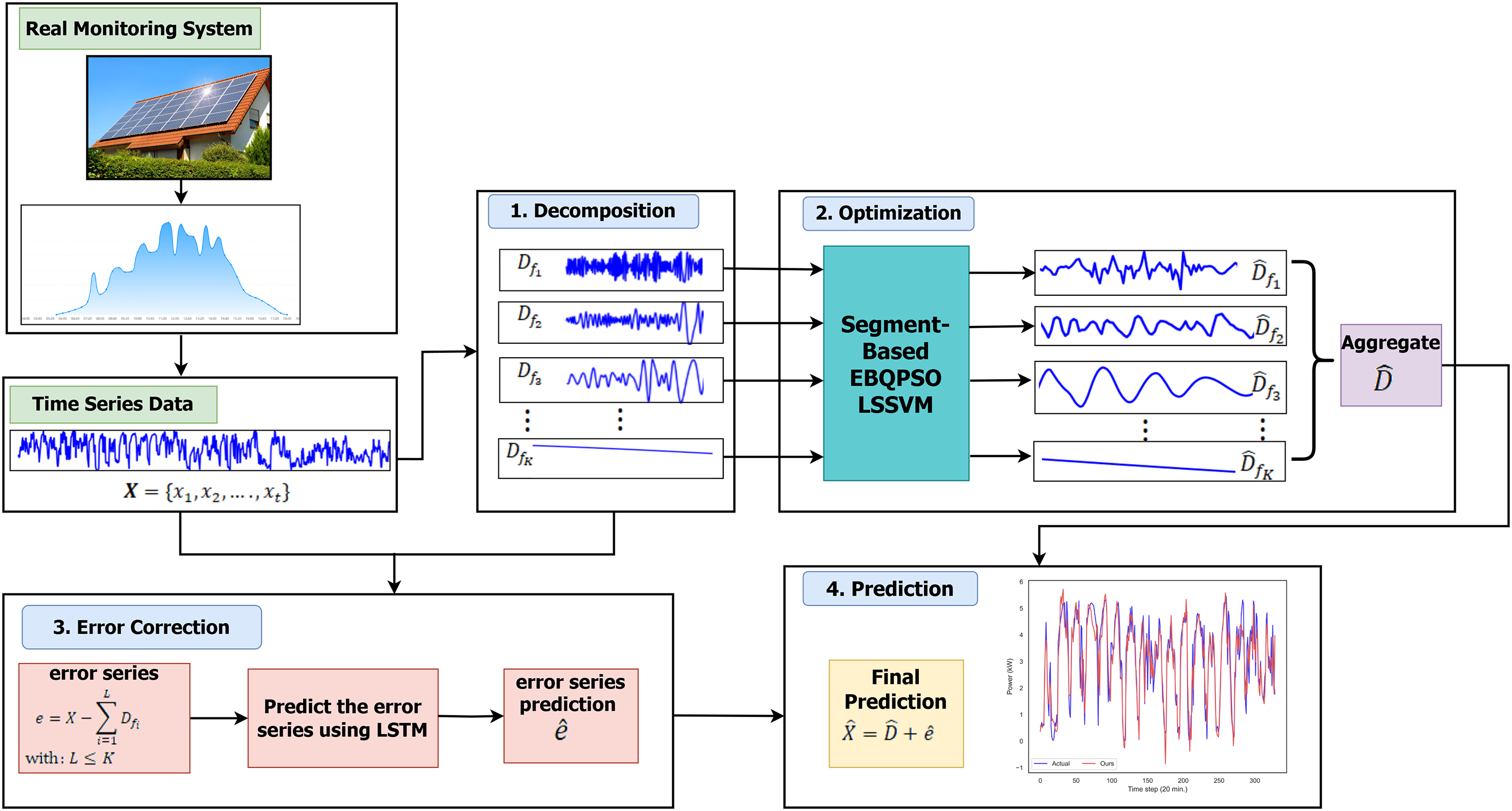
Figure 1: Flowchart of the proposed framework.

The PV power time series first undergoes a preprocessing stage to ensure data continuity and reliability. Missing values are handled using two imputation strategies. Isolated missing points are filled by averaging neighboring observations within a predefined time window to preserve local signal continuity. For contiguous missing segments, a derivative based dynamic time warping interpolation method is applied. This approach reconstructs missing segments by identifying other portions of the time series with similar change patterns. To avoid excessive signal distortion, only gaps with lengths shorter than 30% of the total dataset are reconstructed. After preprocessing, the original PV power series is decomposed into multiple subsignals using CEEMDAN, enabling the extraction of local patterns across different temporal scales. The dataset is then partitioned using a single chronological train–test split without randomization to preserve temporal dependency. During the optimization stage, 50% of the data are used for training, while the remaining data are evenly divided into 25% for validation and 25% for testing.

Each decomposed subsignal is subsequently modeled using the Least Squares Support Vector Machine (LSSVM), with its hyperparameters optimized through the proposed Segment-based Elitist Breeding Quantum-behaved Particle Swarm Optimization (EBQPSO) algorithm. This optimization strategy is designed to improve search efficiency and accelerate convergence under non-stationary conditions. The initial predictions generated from all subsignals are then aggregated to form an intermediate forecast. In the error correction stage, the residual series is computed as the difference between the original PV power signal and the aggregated subsignal predictions. This residual series is modeled using a LSTM network within a residual learning framework to capture high-frequency dynamics and short-term temporal dependencies not addressed by the preceding models. At this stage, 60% of the data are allocated for training, while the remaining 40% are evenly divided into 20% for validation and 20% for testing. All data splits strictly preserve temporal order to prevent information leakage from future observations. A practical challenge during the aggregation process arises from variations in window sizes between subsignal predictions and the residual series, which may lead to length mismatches. This issue is resolved by aligning all prediction sequences to the maximum window size, ensuring consistent aggregation across all components. Finally, the reconstructed residual predictions are added to the aggregated LSSVM output to generate the final PV power forecast. Detailed descriptions of each module within the DOEP framework are provided in the following subsections.

3.1 Decomposition

The datasets consist of time-series data can be described as X={x(1),x(2),…,x(t)}, with xt represents the power output at time t. Let x(t) be the original signal, which is decomposed into IMF using CEEMDAN [14], as described in Eq. (1).

x(t)=∑j=ikIMFj(t)+rK(t)(1)

Each IMF exhibits a specific oscillatory nature that satisfies two conditions. The first condition specifies that the difference between the numbers of local extrema and zero crossings in an IMF must not exceed one. The second condition requires the mean of the upper and lower envelopes to be approximately zero at each time step. In CEEMDAN, each IMF is derived by averaging the ensemble IMF obtained from multiple realizations of the signal [14], as shown in Eq. (2).

IMFk(t)=DfK(t)=1I∑i=1IEk−1(rk−1(t)+εk−1(w(i)(t)))(2)

where: DfK is the result of the k-th signal decomposition, Ek−1(.) is the first IMF extraction operator using EMD, rk−1(.) is residual signal, εk−1(.) is the adaptive noise coefficient that decreases as the IMF index increases, and w(i)(t) is standard white Gaussian noise with mean = 0, standard deviation = 1.

The decomposition process using CEEMDAN produces more stable and consistent IMF due to the addition of adaptive noise and updated ensemble averaging. Thus, after applying adaptive decomposition to the original signal, we obtain the decomposed dataset, defined as: D={Df1,Df2,Df3,…,Df9}, where each Dfk represents a time series data at time t. The decomposed components can be arranged in matrix form as shown in Eq. (3).

D=[Df1(1)Df1(2)⋯Df1(t)Df2(1)Df2(2)⋯Df2(t)⋮⋮⋱⋮Dfk(1)Dfk(2)⋯Dfk(t)](3)

where the k-th row correspond to the k-th decomposed signal, and the j-th column represents the value at time t=j, making D matrix has dimensions of k×t.

3.2 Optimization

The optimization phase involves training each subsignal predicted by LSSVM. Let the training data be represented by T={(xi,yi),yi∈Rm,i=1,2,3,…,N}, with N is the size of the training data and m is the number of input features [30]. By defining and solving the following problems in Eq. (4).

minJ(w,e)=12(w⊤w+γ∑i=1Nei2)subject to:yi=w⊤ϕ(xi)+b+ei,i=1,2,…,N(4)

where w and b are the weights and bias, respectively, ei is the error of the i-th sample, γ is the regularization parameter, and ϕ(xi) denotes the nonlinear mapping of the input xi into a high-dimensional feature space. Based on Eq. (4), this optimization problem can be solved using Lagrange multipliers and satisfies the Karush-Kuhn-Tucker (KKT) conditions [30], so the LSSVM regression function can be written as shown in Eq. (5).

f(x)=∑i=1NaiK(x,xi)+b(5)

with K(x,xi) is a kernel function. In this research, the Gaussian RBF kernel function is used, which is: K(x,xi)=exp⁡(−(x−xi)22σ2), where σ is the kernel parameter.

To determine the optimal hyperparameters of the LSSVM model, such as the regularization parameter (γ), kernel parameter (σ), and window size (m), a segment-based EBQPSO algorithm is employed. Fig. 2 presents the flowchart of the segment-based EBQPSO algorithm.

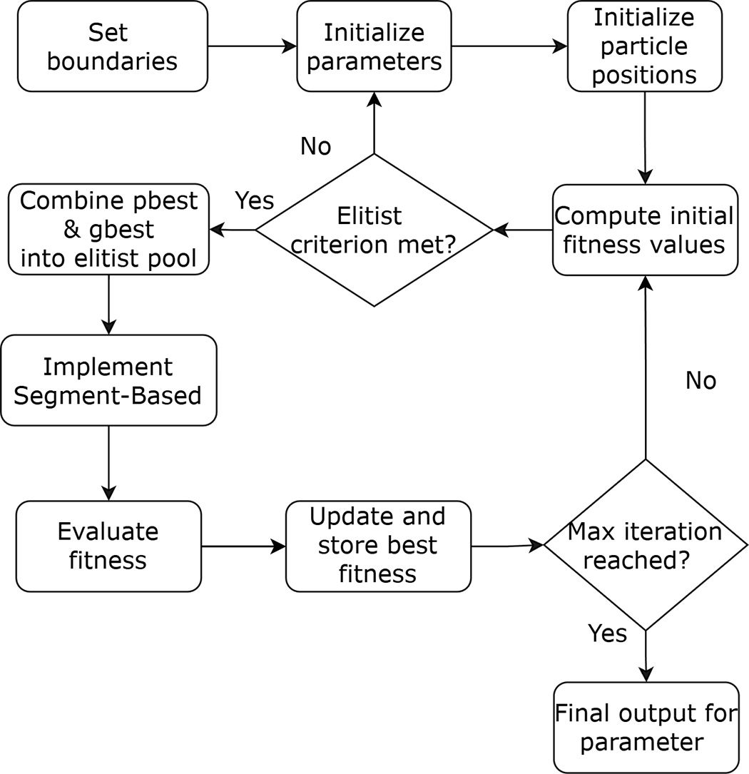
Figure 2: The schematic workflow of proposed segment-based EBQPSO algorithm.

As illustrated in Fig. 2, the algorithm begins by setting boundary values as initial parameters. Each particle in the population is randomly initialized within the lower and upper bounds of the search space. The new position of each particle xi is updated based on the quantum delta potential well model, using the gravitational center of the particle called the attractor point pi, which is calculated from the personal best (pbesti) and global best (gbest) combined. The position update formula is defined in Eq. (6) [47].

zi=pi±b.|xi(t)−mbest|ln⁡(1u)(6)

with pi is the attractor point based on individual and global exploration as presented in Eq. (7) [47].

pi=c1.fi.pbesti+c2.(1−fi).gbestic1+c2(7)

where c1 and c2 are weighting coefficients or learning factors that control the relative contribution of the two important components in updating the particle’s position, and fi∼U(0,1) is a random number for interpolation between pbest and gbest. In Eq. (6), b is the quantum spread, mbest is the average best position of all particles, and u∼U(0,1) is a random number from a uniform distribution. The direction (+ or −) is chosen randomly with a 50% probability. From Eq. (8), α is an adaptive scaling parameter that decreases linearly with iteration, so the quantum spread is expressed as shown in Eq. (8) [47].

b=α.|zi(t)−mbest|(8)

with mbest=1n∑j=1npbesti

To enhance solution diversity and avoid local minima, the algorithm incorporates elitism and segment-based transposon operators. Transposons based-segments between solutions in the elitism pool, mimicking biological evolution to introduce variation. Before segment exchange, all individuals in the elitism pool are normalized to [0, 1] element-wise to ensure consistent scaling across dimensions [47], using the equation Eq. (9).

z′=z−zminzmax−zmin(9)

The normalization ensures that the values between dimensions or individuals, which may vary greatly in scale, are proportional for segment exchange. The minimum and maximum values, zmin and zmax, are used to normalize each element z within the population. After normalization, the transposon operator randomly selects two individuals, c1 and c2, from the elitism pool. A fixed-length segment is cut from each individual by randomly selecting initial segment indices (d1 and d2) from the dimension range and s is segment length as indicated in Eq. (10).

seg1=z′[d1:d1+s]andseg2=z′[d2:d2+s](10)

The segments are exchanged between individuals, mimicking cut-and-paste transposons in genetics, creating local variations without disrupting overall solutions. By limiting segment length, this acts as a local repair or microinformation exchange, preserving promising solution structures. Afterward, all individuals are denormalized to their original scale described in Eq. (11).

z=z′.(zmax−zmin)+zmin(11)

This step restores solutions to valid values within the optimization domain for objective evaluation and updates. After applying the transposon operator, each elite individual (eliti) is compared to its previous personal best pbesti. If eliti has a lower objective value, pbesti is updated. This elitism check ensures solution quality, after which all pbesti values are recalculated to determine the global best (gbest) as the individual with the lowest objective value. This mechanism balances exploration and elite preservation, preventing solution quality degradation and premature convergence. The algorithm combines probabilistic QPSO, dynamic parameter adaptation, and a transposon operator to improve convergence while maintaining population diversity, iterating until the maximum iteration limit is reached to obtain the optimal solution.

In this optimization stage, the regularization parameter (γ), kernel parameter (σ2), and window size (m) is optimized by Segment-based EBQPSO algorithm for each mode of the decomposed series. The optimization process begins by initializing the particle population, where each particle represents a combination of parameters (γ, σ2, m). Each particle has a position and velocity in the search space. The position corresponds to the parameter values being tested, while the velocity controls the particle’s movement within the search space. Each particle is evaluated by calculating the fitness or performance of the selected parameter combination. In this case, fitness is computed based on the mean square error on the validation data, which measures how well the model can predict the data. The LSSVM model is trained using the parameters provided by the particle, and its predictions are compared to the target values to obtain the MSE. At each iteration, Segment-based EBQPSO searches for the optimal values of the parameters γ, σ2, and m. Here, m determines the window size used to form the input features from the time series data. The optimized value of m plays a crucial role in defining the time window length for processing the data using a sliding window approach. The optimization results for m across each IMF from the decomposition are stored in an array, and the largest window size value is selected as the optimal value to be used throughout the model. This optimization is crucial, as an appropriate window size enables more effective capture of temporal patterns, leading to improved prediction accuracy on unseen data. Optimizing m ensures that the chosen time window effectively captures relevant temporal patterns while avoiding noise and overfitting. Optimizing the window size is a crucial step in the feature extraction process for time-series forecasting. In this pipeline, the window size is optimized using the Segment-based EBQPSO algorithm for each mode generated by CEEMDAN, and the optimized windows are subsequently used in LSSVM for training and prediction. This process ensures that the model is trained on features that are well aligned with the temporal patterns in the data, capturing both long-term and short-term dynamics while avoiding overfitting on the training data.

3.3 Error Correction

At the error correction stage, the error series is predicted using the LSTM model. The combination process involves summing between 2 to K−1 subsignals IMF, then calculating the error between the sum of the combined signals and the original data using Eq. (12). The error series with the lowest mean square error is selected as the optimal series. This series is the input for the LSTM model.

e=X−∑i=1LDfi(12)

Here, L denotes the number of selections from combinations of 2 to K−1 and X is original data and Dfi is the decomposed signal corresponding to fi. Each LSTM unit consists of three gates: input, output, and forget gate. Specifically, the forget gate controls which information from the previous state is removed. The LSTM architecture is illustrated in Fig. 3.

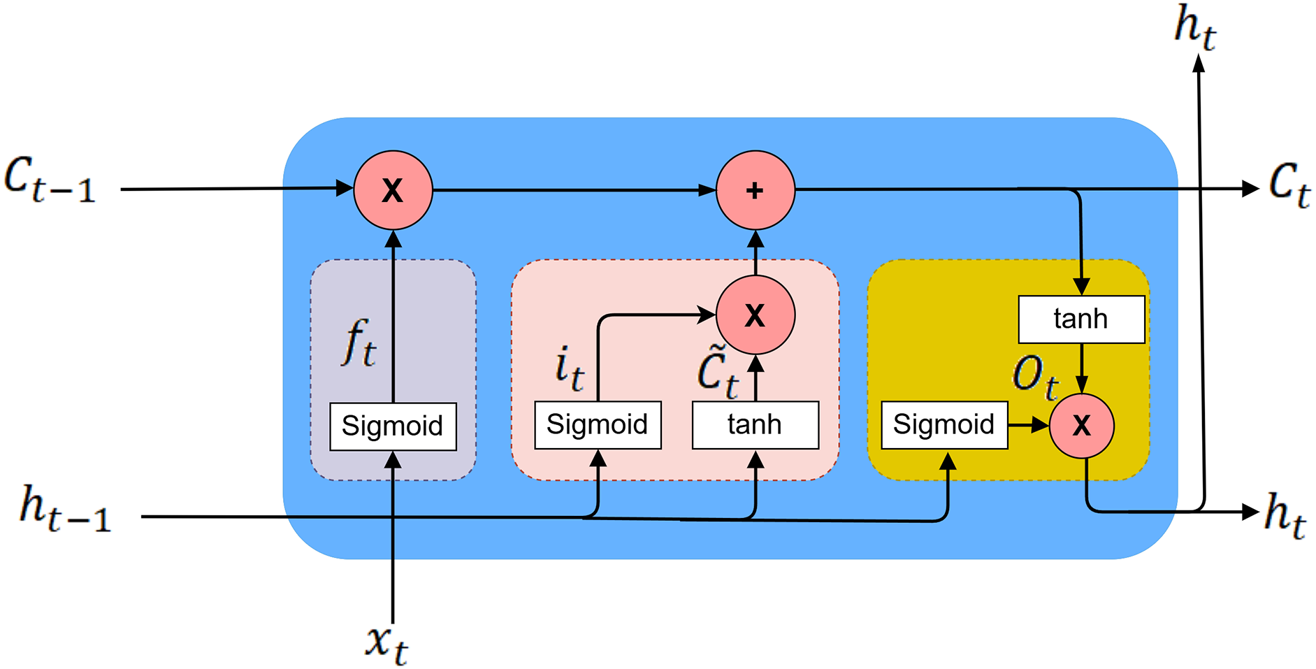
Figure 3: LSTM architecture used for error series modeling.

The computations in LSTM are determined using mathematical formulations presented in Eq. (13) [26].

ft=sigmoid(Wf⋅[ht−1,Xt]+bf)it=sigmoid(Wi⋅[ht−1,Xt]+bi)C~=sigmoid(WC⋅[ht−1,Xt]+bC)C=ft⊙Ct−1+it⊙C~Ot=sigmoid(Wo⋅[ht−1]+bo)ht=Ot⊙tanh⁡(Ct)(13)

With ft, it, C~ and Ot are the activation of the forget, input, cell state, and output gates, respectively, Wf, Wi, WC, and WO are the corresponding weight matrices and bf, bi, bc, and bo are bias vectors. The cell state at time t are given by Ct and ht, respectively. The operator ⊙ denotes element-wise multiplication, while σ(⋅) and tanh⁡(⋅) indicate the sigmoid and hyperbolic tangent activation functions.

3.4 Prediction

At the prediction stage, the final forecast is obtained by concatenating the initial prediction with the error series predictions. The initial prediction is derived by aggregating the forecasts of each decomposed signal at time t, which can be expressed as: D^={D^f1,D^f2,D^f3,…,D^fk} with each D^fk consist of series data at time t. The aggregated predictions can be represented in matrix form in Eq. (14).

D^=[D^f1(1)D^f1(2)⋯D^f1(t)D^f2(1)D^f2(2)⋯D^f2(t)⋮⋮⋱⋮D^fk(1)D^fk(2)⋯D^fk(t)](14)

By aggregating the predictions from each decomposed signal in Eq. (14), the initial forecast time series can be written as D^=D^(1),D^(2),…,D^(t). From the error correction stage, the predicted error series is obtained as e^=e^(1),e^(2),…,e^(t). The final forecast of the PV power output is then obtained by concatenating the subsignal predictions and error predictions at each time t, can be written in Eq. (15).

X^=D^+e^(15)

4  Result and Discussion

This section presents the data acquisition, the results of signal decomposition and correlation analysis, performance evaluation of the Segment-based EBQPSO on benchmark function, experimental and parameter setting, comprehensive analysis, the ablation study of the proposed framework, and the performance comparison of the proposed framework with benchmark methods.

4.1 Data Acquisition

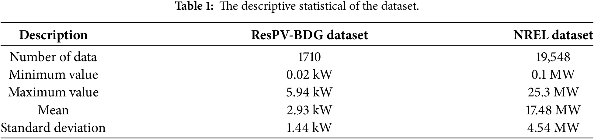
All experiments were performed on a system with a 13th Gen Intel® Core™ i5-13600KF processor at 3.50 GHz, and the models were implemented using Python 3.12.7. This study uses two datasets. First, the ResPV-BDG dataset was collected from a residential PV monitoring system in Bandung, Indonesia [51]. The data were recorded at 20-min intervals from January 1 to March 31, 2023. Second, the NREL dataset was obtained from the National Renewable Energy Laboratory (NREL) in Arizona region from January 1, 2006, to March 31, 2026, at 5-minute intervals [52]. The descriptive statistics of the datasets are described in Table 1.

4.2 Results of Signal Decomposition and Correlation Analysis

The original dataset was decomposed using the CEEMDAN method, as shown in Fig. 4, there are 9 subsignals for the ResPV-BDG dataset, denoted as Df1,Df2,…,Df9. Each IMF represents a distinct frequency component, ranging from high to low. Df1 captures the highest frequency, corresponding to noise or rapid fluctuations. Df2 to Df4 represent mid to high frequencies, reflecting intermediate oscillations such as daily or weekly patterns. Df5 to Df7 capture medium to low frequencies, indicating trends, seasonality, or systematic patterns. Df8 to Df9 represent the lowest frequencies, capturing long-term trends or gradual changes. The NREL dataset has 15 subsignals, denoted as Df1,Df2,…,Df15.

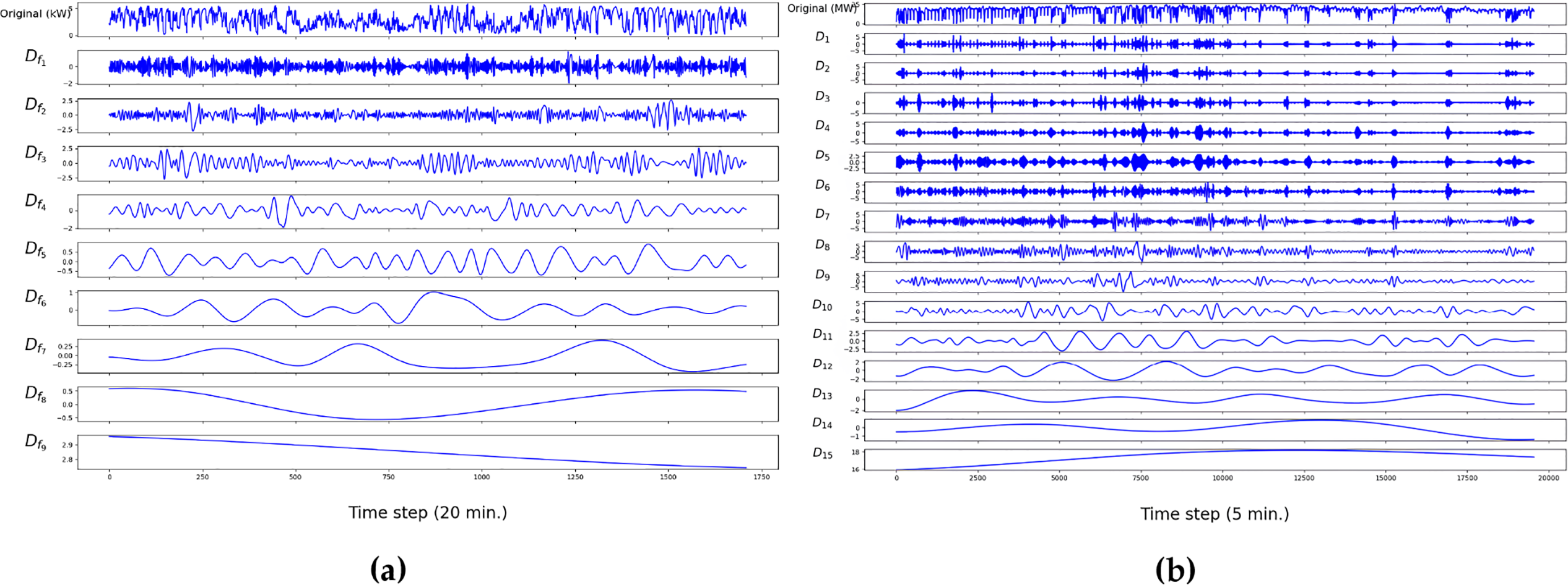
Figure 4: Signal decomposition for: (a) the ResPV-BDG dataset; (b) the NREL dataset.

The correlations between the decomposed components were analyzed to evaluate the effectiveness of the decomposition process. Spearman’s rank correlation coefficients were applied to examine whether the CEEMDAN algorithm successfully separated the PV power series into independent subsignals, each characterized by distinct and uniformly distributed center frequencies. As shown in Fig. 5, the highest correlation value observed was 0.20 for the subsignal Df7 in the ResPV-BDG dataset and 0.20 for the subsignal Df14 in the NREL dataset. In contrast, the remaining subsignals showed very low or negative correlations, suggesting that they are largely uncorrelated. This outcome implies that the IMF components are independent and well separated, with negative correlations further highlighting significant frequency discrepancies. Collectively, these findings substantiate the effectiveness of CEEMDAN in successfully decomposing the original PV power signal into independent sub-components.

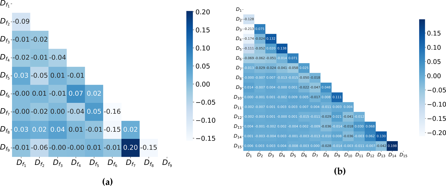
Figure 5: Correlation matrix for: (a) the ResPV-BDG dataset; (b) the NREL dataset.

Based on the decomposition results, the error series is constructed using Eq. (12). The selected signal combination that has the lowest mean square error (MSE) are Df1,Df2,Df3,Df4,Df5,Df6,Df8 for the ResPV-BDG dataset and Df1,Df2,Df3,Df4,Df5,Df6,Df7,Df8,Df9,Df10,Df11,Df12,Df13,Df15 for the NREL dataset. The lowest MSE values are 0.1836 and 0.6204 for the ResPV-BDG dataset and the NREL dataset, respectively. So, the error series is constructed from the differences between the original data and the selected signal combination, and this error series is used as input to the LSTM.

4.3 Performance Evaluation of the Segment-Based EBQPSO for Benchmark Function

The performance of the segment-based EBQPSO algorithm was assessed and compared with EBQPSO, QPSO, and PSO using four benchmark functions: the Sphere Function (G1), Ackley Function (G2), Griewank Function (G3), and McCornick Function (G4). Each algorithm was evaluated on these functions through 30 trials to generate confidence intervals and evaluate their relative performance. The dimensionality (d) for each function was set to d = 20 for G1, G2, and G3, but d = 2 for G4. The mathematical formulas for the benchmark functions are provided in Eq. (16).

G1(x)=∑i=1dxi2G2(x)=−20e−0.21d∑i=1dxi2−e1d∑i=1dcos⁡(2πxi)+20+eG3(x)=∑i=1dxi24000−∏i=1dcos⁡(xii)+1G4(x)=sin⁡(x1+x2)+(x1+x2)2−1.5x1+2.5x2+1(16)

The sensitivity analysis was evaluated on the grid parameters of the segment-based EBQPSO algorithm by examining multiple parameter configurations. The segment length was varied within the range [1, 2, 3], the jumping rate within [0.1, 0.2, 0.3], the population size within [5, 10, 25], and the number of generations within [50, 100]. Based on 30 independent runs, the configuration consisting of the segment length of 3, the jumping rate of 0.3, the population size of 25, and 100 generations achieved the lowest mean best fitness value. The comparative results of the 30 runs are described in Table 2. For function G1, the Segment-based EBQPSO achieves results very close to the global minimum value (0), with a very small standard deviation, indicating stable and consistent performance. In contrast, PSO produces significantly higher values, demonstrating lower effectiveness for this function. A similar trend is observed for function G2, where Segment-based EBQPSO again yields results near to 0, while PSO reports much larger values. For function G3, Segment-based EBQPSO outperforms both QPSO and EBQPSO, while PSO produces notably higher values, indicating poor performance on this function. For function G4, whose global minimum is −1.9132, both Segment-based EBQPSO and EBQPSO return values very close to the optimum with small standard deviations, reflecting high stability. In contrast, PSO again performs poorly, with results far from the ideal value.

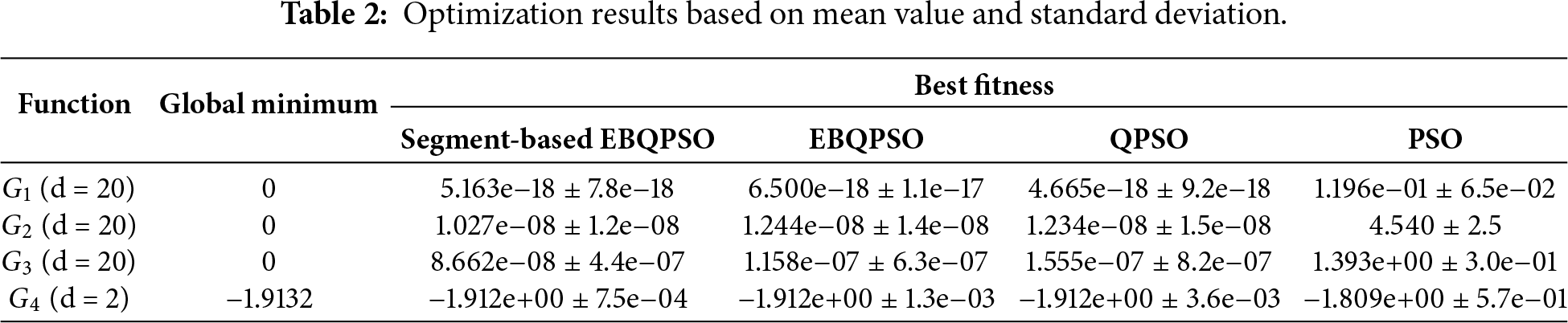
Fig. 6 shows the convergence curve for the Sphere function to find the best fitness using the Segment-based EBQPSO algorithm compared to EBQPSO, QPSO, and PSO. The PSO exhibits the slowest convergence, indicating a limited exploitation efficiency in the classical velocity-update mechanism. The QPSO improves the convergence rate via quantum-behaved search dynamics, though performance gains diminish after the initial iterations. The EBQPSO further enhances the stability and speed of convergence through elitist breeding, promoting the exploitation of high-quality solutions. The Segment-EBQPSO achieves the fastest and most stable convergence, characterized by a rapid reduction in the best fitness value from the initial iterations. This improvement is attributed to the segment-based transposon operator, which facilitates effective exchange of structural information among elite particles, thereby accelerating the exploitation and mitigating premature stagnation.

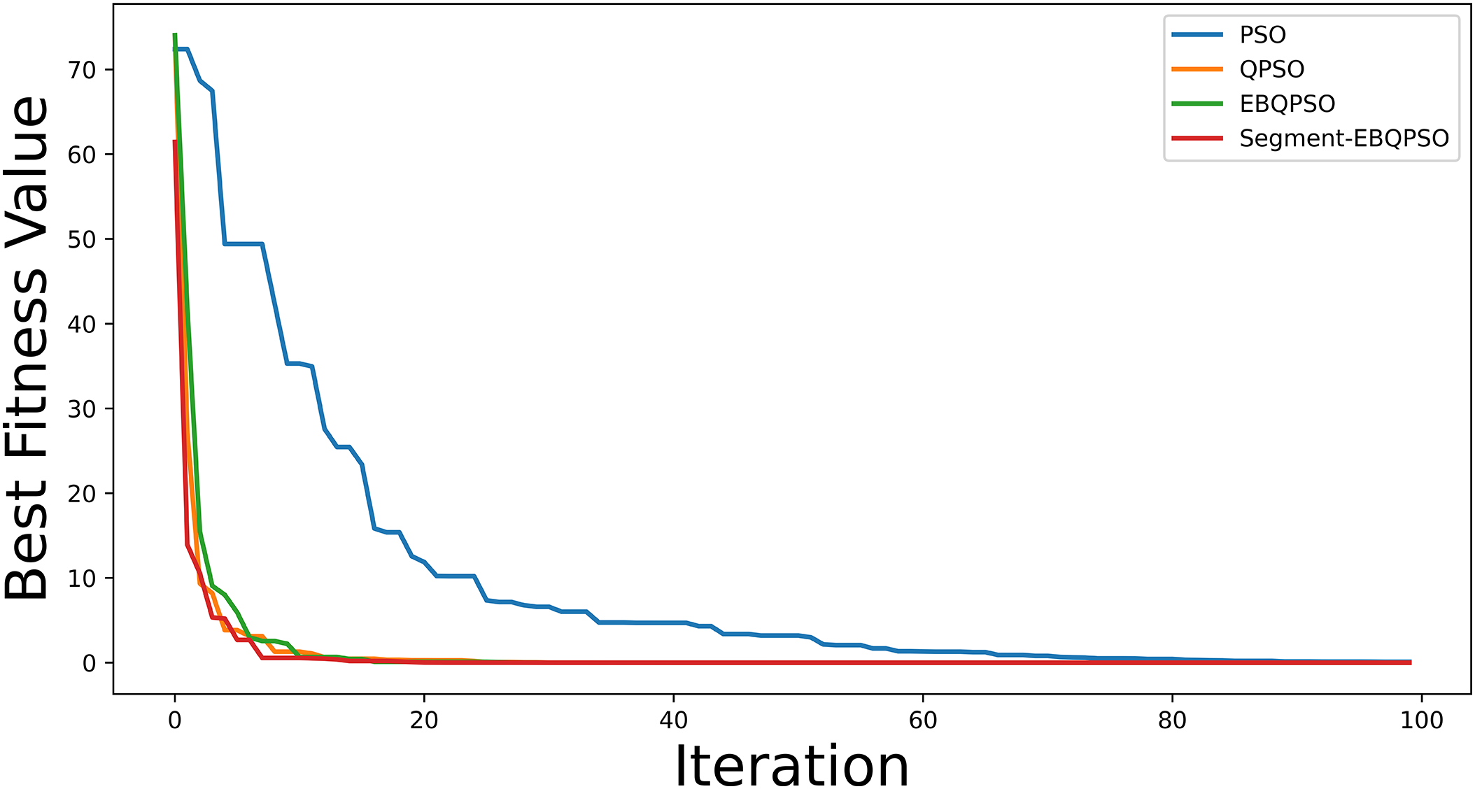
Figure 6: Convergence curve for the Sphere function.

Overall, the Segment-based EBQPSO consistently provides the most stable results and closely approximates the global minimum across most benchmark functions, while PSO exhibits significantly inferior performance, characterized by larger standard deviations from the optimal values. Given its superior convergence behavior and robustness across diverse test functions, the Segment-based EBQPSO was selected as the optimization engine to adjust the hyperparameters of the LSSVM model and determine the optimal window size for each component in the proposed framework.

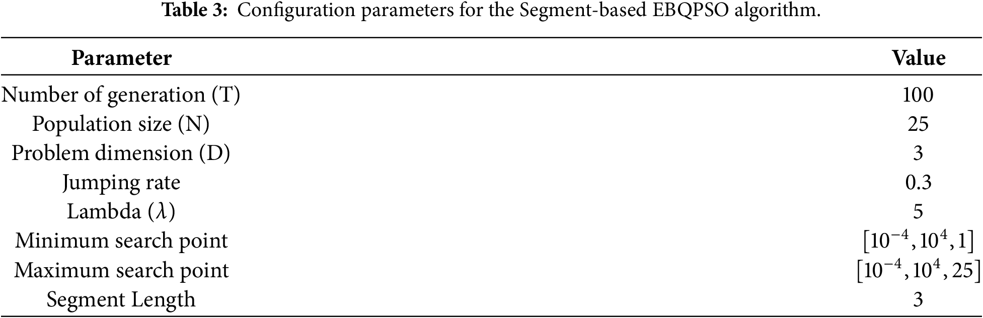
In the optimization stage, LSSVM hyperparameters and the window size of each component were optimized using the Segment-based EBQPSO algorithm. Table 3 presents the parameter settings for the Segment-based EBQPSO algorithm based on the grid parameter results. The algorithm was configured to run for a maximum of 100 generations with a population size of 25. Since three hyperparameters were optimized, the problem dimension was set to 3. The jumping rate in the Segment-based EBQPSO algorithm with segment transposons is a probabilistic parameter that governs how often an individual in the elitism pool will be subjected to the transposon operator. Its value is in the range [0,1]. The jumping rate value of 0.3 indicates that applying the segment transposon to each individual in the elitism pool with a chance of 30%, and the swapped segment has a length of 3. The value of λ is set to 5 to trigger the elitism process every 5 generations. The determination of the search space is also very important: the minimum value for γ and σ2 which are LSSVM parameters is set at 0.0001 and the maximum at 10,000. The window size ranges from 1 to 25. In addition, the search space for σ2 and γ is mapped on a logarithmic scale to make the search process more efficient and converge faster to the optimal value.

4.4 Ablation Study of the Proposed Framework

Based on the proposed framework, the ablation study was used to evaluate the contribution of each component within the DOEP framework. The proposed framework was evaluated using a comprehensive set of metrics, including Mean Absolute Error (MAE), Mean Square Error (MSE), Root Mean Square Error (RMSE), Mean Absolute Percentage Error (MAPE), Coefficient of Determination (R2), Correlation Coefficient (CC), and Explained Variance Score (EVS). MAE captures the mean absolute deviation between predicted and observed values, while RMSE emphasizes larger errors through squared deviations. MAPE provides a normalized error measure in percentage form. The R2 metric evaluates the proportion of variance explained by the model, CC measures the linear dependence between predictions and observations, and EVS quantifies the fraction of target variance accounted for by the predicted outputs. Below the description for each component in ablation study:

•   Optimization (O): This model employs LSSVM as the baseline predictive model, where the regularization parameter, kernel parameter, and input window size are optimized using the Segment-based EBQPSO algorithm.

•   Decomposition-Error correction (DE): This model was started with adaptive signal decomposition using CEEMDAN. Each decomposed subsignal is predicted independently using LSSVM with fixed parameter settings, and the resulting forecasts are combined to form an initial prediction. Subsequently, the error correction stage computes the residual by taking the difference between the original signal and the reconstructed signal derived from adaptive decomposition. This residual sequence is then modeled using an LSTM network. Finally, the predicted residual is incorporated into the initial forecast to obtain the final prediction

•   Decomposition-Optimization (DO): The model begins with adaptive decomposition using CEEMDAN. Each subsignal is predicted using LSSVM, with its parameters optimized by the Segment-based EBQPSO algorithm. Finally, the predictions of all subsignals are aggregated to generate the overall PV power output forecast.

•   Decomposition-Optimization-Error correction-Prediction (DOEP): The proposed framework starts with the adaptive decomposition of the original PV signal using CEEMDAN. Each decomposed subsignal is then predicted using LSSVM, with its hyperparameters optimized by the Segment-based EBQPSO algorithm. The predictions of all subsignals are aggregated to produce the initial forecast. For error correction, the difference between the original signal and the reconstructed signal from adaptive decomposition is computed to obtain an error series, which is subsequently predicted using LSTM. Finally, the predicted error series is combined with the initial forecast to generate the final PV power output prediction.

As shown in Table 4, the proposed DOEP framework outperforms all baseline models in every evaluation metric. For the ResPV-BDG dataset, the O model exhibits the highest MSE (0.9959) and RMSE (0.9980), indicating poor predictions. The R2 value of 0.5883 shows that it explains only 58.83% of the variance, reflecting limited accuracy. The CC of 0.7735 indicates a moderate correlation. For the NREL dataset, O performs worse, with an even higher MSE (4.7524) and RMSE (2.18), and a very low R2 (0.5105). The DE model improves slightly over O, with better R2 (0.5716) and CC (0.7681) for the ResPV-BDG dataset, but still shows high MSE (1.0363) and RMSE (1.0180). For the NREL dataset, DE performs better, with MSE (1.5246) and RMSE (1.2347), and a strong R2 of 0.843, but still lags behind DO and DOEP. The DO model shows more substantial improvement, with lower MSE (0.7495) and RMSE (0.8657) for the ResPV-BDG dataset, along with higher R2 (0.6902) and CC (0.9090). For the NREL dataset, DO further improves, achieving R2 (0.8569) and CC (0.9669), indicating strong predictive performance. The DOEP model achieves the best overall performance. For the ResPV-BDG dataset, it yields the lowest MSE (0.4363) and RMSE (0.6605), with the highest R2 (0.8197) and CC (0.9090). For the NREL dataset, DOEP excels even further with the lowest MSE (0.5356) and RMSE (0.7318), and the highest R2 (0.9448), CC (0.9723), and EVS (0.9449).

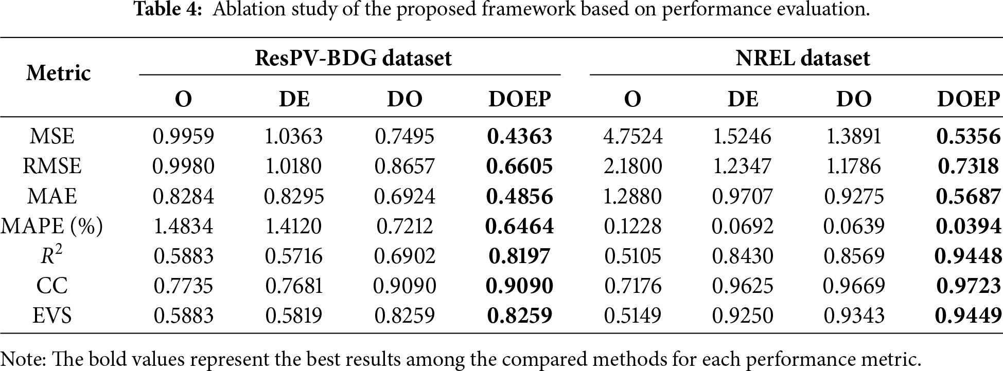
Overall, the DOEP framework consistently exceeds the other models in both accuracy and robustness. By integrating decomposition, hyperparameter optimization, and error correction, the DOEP framework effectively handles the nonlinear and nonstationary nature of PV power data, thereby significantly improving forecast performance. This highlights the effectiveness of combining these steps to address the challenges in the forecasting of PV power.

4.5 Performance Comparison of the Proposed Framework with Benchmark Methods

This section presents the comparison of the proposed framework with six benchmarks methods: CNN, CEEMDAN-CNN, LSTM, CNN-LSTM, CEEMDAN-LSTM, and CEEMDAN-CNN-LSTM. The parameter setting for the benchmark methods for CNN and LSTM can be described at Table 5. The values of selected parameter are utilized to optimize the parameters of hybrid model in the benchmark methods.

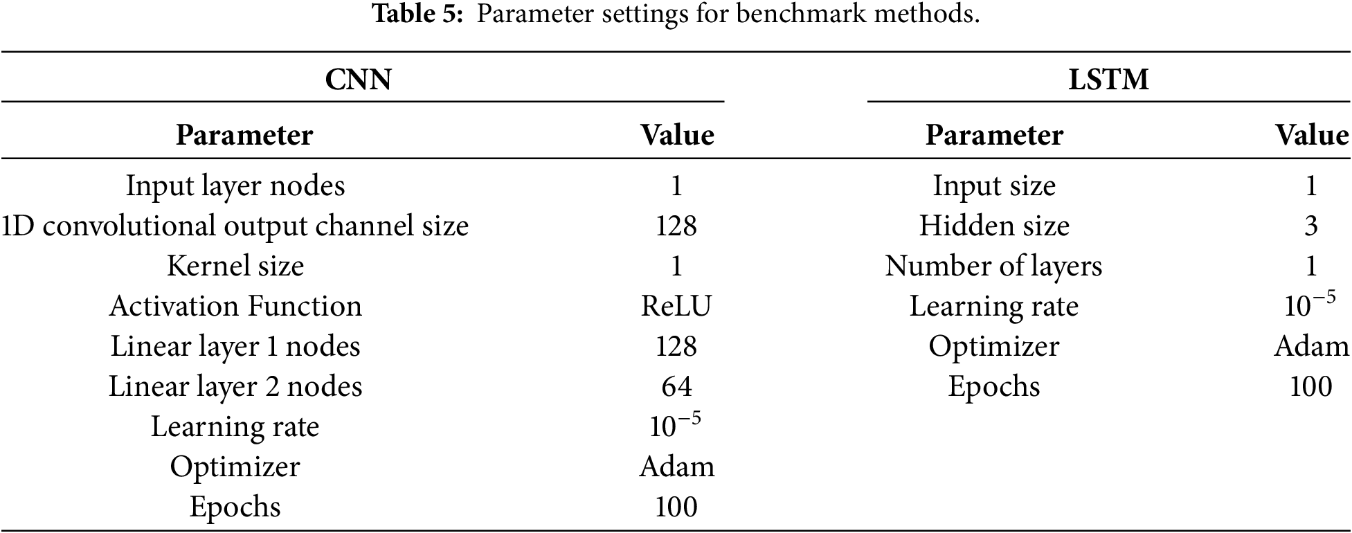
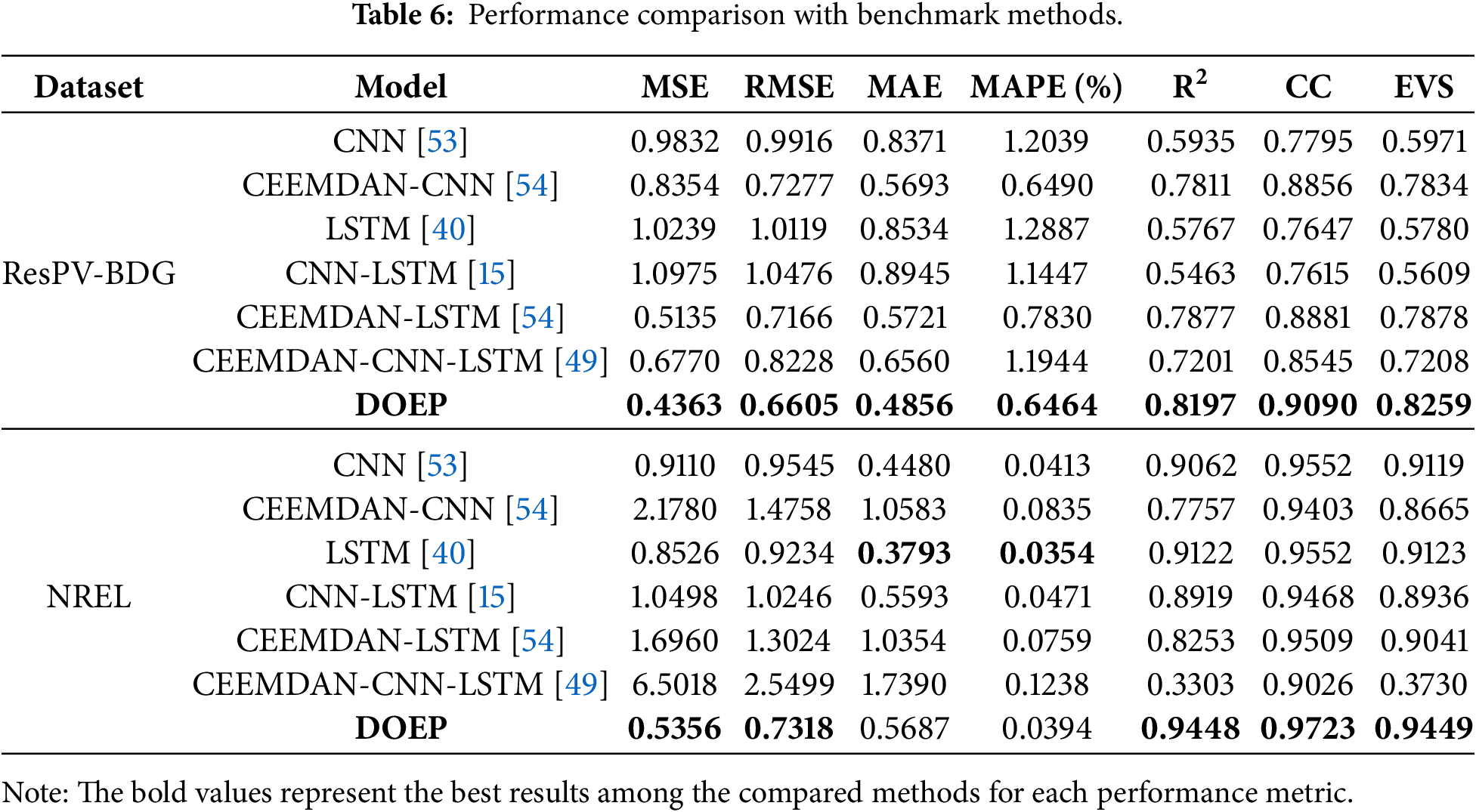
Table 6 presents the proposed DOEP model compared with several benchmark approaches on two datasets using error-based and goodness of fit metrics. The DOEP model outperforms all others, with the lowest MSE (0.4363) and RMSE (0.6605) for the ResPV-BDG dataset, and MSE of 0.5356 and RMSE of 0.7318 for the NREL dataset. It also achieves the highest R2, CC, and EVS values, demonstrating superior accuracy and robustness. This model significantly outperforms the others by incorporating the strengths of CEEMDAN for decomposition, LSSVM for prediction, Segment-based EBQPSO for hyperparameter optimization, and LSTM for error correction. The DOEP framework demonstrates excellent performance in terms of accuracy, robustness, and adaptability, making it a promising solution to predict PV power output. The addition of error correction through LSTM further enhances the model’s ability to handle residual errors, contributing to the overall accuracy of the forecast. So, the DOEP model proves to be a comprehensive and effective approach for forecasting PV power output, addressing key challenges related to nonstationary, nonlinear, and noisy data. The proposed framework integrates advanced techniques in decomposition, optimization, error correction, and prediction to deliver precise forecasts, positioning it as an essential tool for solar energy forecasting and seamless integration into the power grid.

Linear fit is a key indicator for evaluating forecasting performance, where an ideal model produces predictions that align exactly with observed values, resulting in a slope of one. In general, a strong fit is indicated by the proximity of the predicted values to the actual ones. Thus, the effectiveness of the model can be gauged by how closely the predicted points align with the linear line and by the value of its slope. In Fig. 7, the linear fit graphs of the DOEP model and the benchmark methods applied to the ResPV-BDG dataset are presented. These include graphs that compare actual vs. predicted values, the linear line, and its corresponding linear equation, written as y=mx+b, with m is the slope and b is the y-intercept. For the ResPV-BDG dataset, most benchmark models exhibit regression slopes far below 1 (approximately 0.47–0.76), indicating that their predictions tend to compress the range of values. Specifically, when the actual values are high, the models tend to underpredict, whereas when the actual values are low, they may overpredict also reflected by relatively large intercepts. In contrast, DO and DOEP achieve the highest slopes (around 0.85), suggesting that their prediction scales are closer to actual patterns. Moreover, DOEP follows the trend more closely, indicating greater stability.

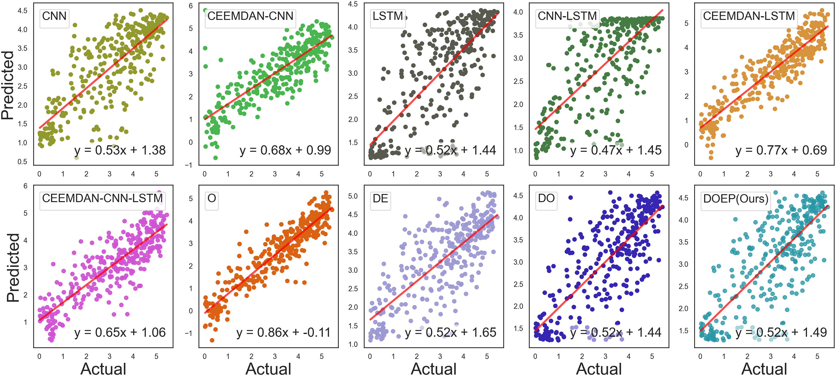
Figure 7: Linear fit of actual and predicted data for the ResPV-BDG dataset.

Based on Fig. 8, DOEP shows the best calibration using the NREL dataset, with prediction points more closely aligned with the regression line and a slope close to 1 (approximately 0.93). In contrast, poorly performing models exhibit clear miscalibration patterns. For example, O shows a low slope (around 0.52) combined with a large intercept, indicating weak predictive sensitivity, where predictions tend to lock within a narrow range. Meanwhile, CEEMDAN-CNN-LSTM presents a slope greater than 1 (around 1.41), signaling severe miscalibration and instability, which is consistent with its poor boxplot distribution and performance metrics.

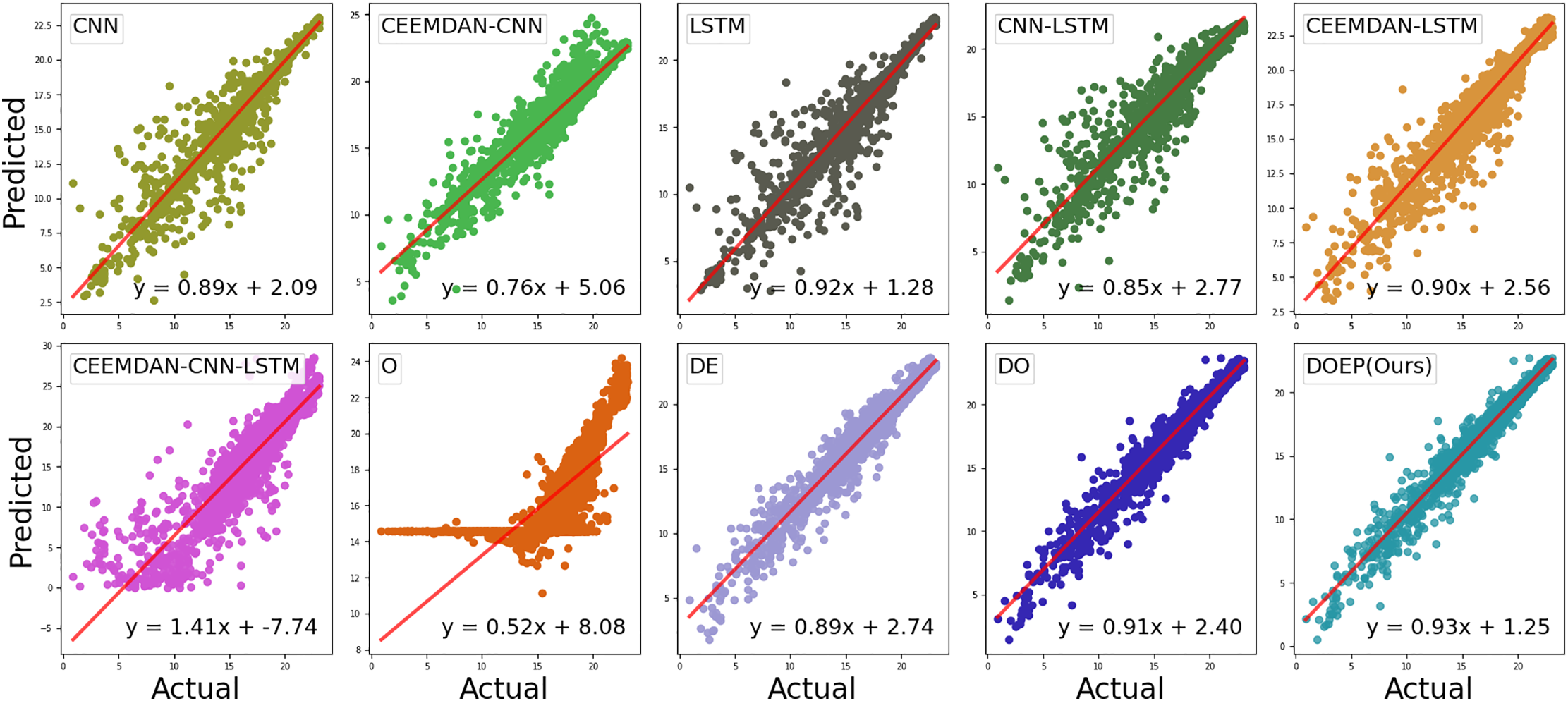
Figure 8: Linear fit of actual and predicted data for the NREL dataset.

Fig. 9 presents the boxplot distribution of residual errors for the ResPV-BDG dataset across all benchmark models and the proposed DOEP framework. In this plot, good performance is indicated by residuals centered around zero, a narrow interquartile range (IQR), short whiskers, and fewer extreme outliers. The baseline CNN, LSTM, and CNN-LSTM models exhibit relatively wider IQRs and longer whiskers, reflecting higher variability in prediction errors when PV output fluctuates. Although the CEEMDAN-CNN model benefits from signal decomposition, it still shows several extreme negative outliers, suggesting occasional underestimation. In contrast, CEEMDAN-LSTM and CEEMDAN-CNN-LSTM produce more compact residual distributions, implying improved stability from combining decomposition with temporal learning. Among all approaches, DOEP yields the most concentrated residuals near zero with a comparatively smaller spread and fewer extreme deviations, indicating lower bias and more consistent forecasting behavior on the ResPV-BDG dataset.

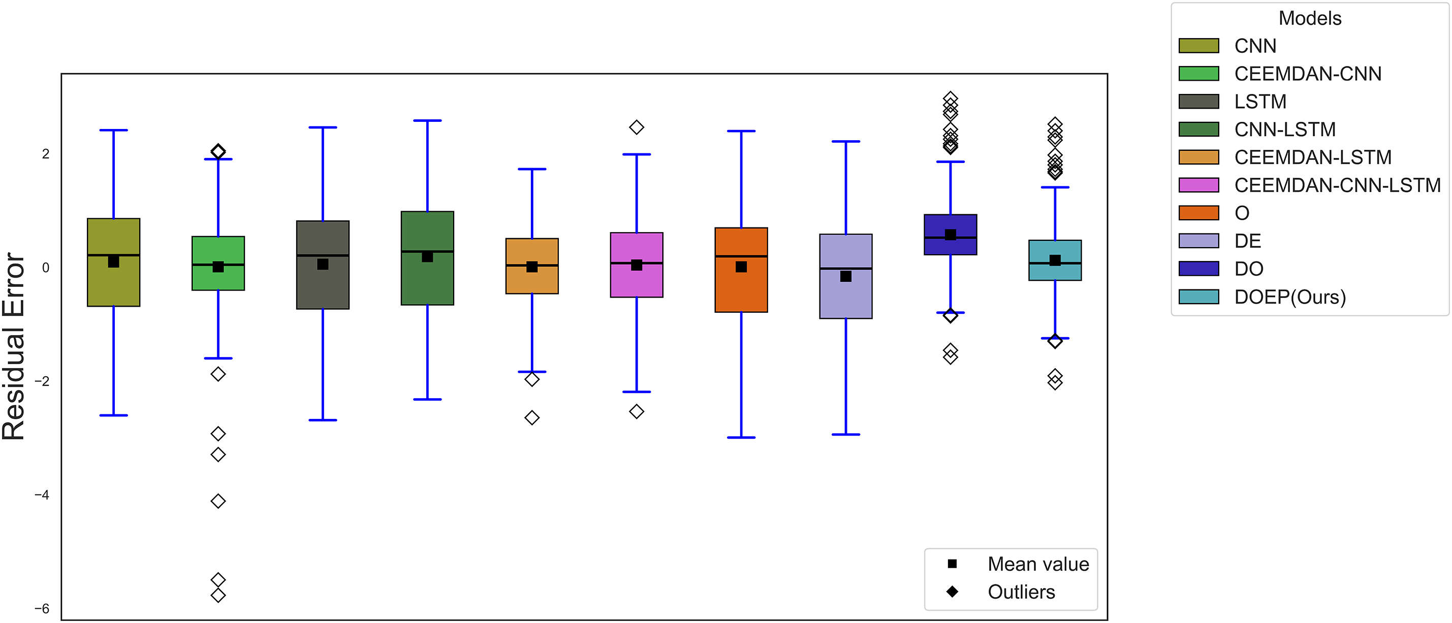
Figure 9: Boxplot distribution of residual error for the ResPV-BDG dataset.

Fig. 10 presents the boxplot distribution of residual errors for the NREL dataset. Baseline models such as CNN and LSTM display highly dispersed residuals with many outliers on both the positive and negative sides, indicating unstable errors under rapid PV ramps or irregular patterns. Decomposition-based hybrids (CEEMDAN-CNN and CEEMDAN-LSTM) tend to improve the central tendency of residuals, but they still exhibit numerous outliers and a wide spread, meaning their stability remains suboptimal on the NREL dataset. The most pronounced degradation is observed for CEEMDAN-CNN-LSTM, which shows the largest dispersion and extremely high positive outliers, indicating severe overestimation events and weak generalization on this dataset. Meanwhile, the O model presents very extreme negative outliers, reflecting occasional large underestimation. Compared with other methods, DOEP (Ours) maintains residuals that are more tightly concentrated near zero with a relatively smaller IQR and more controlled outliers, demonstrating better robustness and prediction consistency on the NREL dataset. This result align with the goodness of fit metrics in Table 5, which confirm that DOEP remains more stable under more complex data conditions.

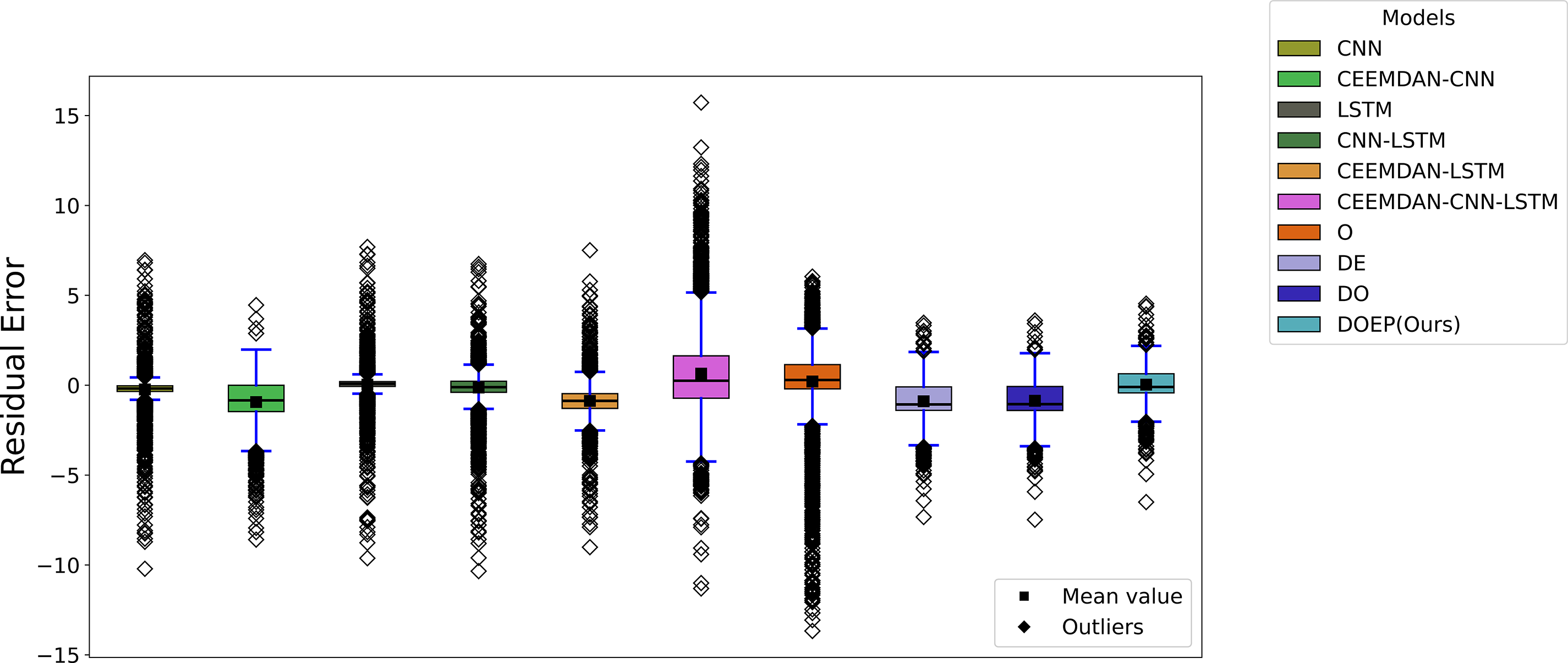
Figure 10: Boxplot distribution of residual error for the NREL dataset.

Table 7 reports the computational time required by each method in the NREL dataset, highlighting the trade-off between the accuracy of the forecasting and the computational cost. The O model achieves the shortest runtime because it relies on a single model and a relatively simple training evaluation pipeline. In contrast, the proposed DOEP framework requires substantially more computational time, mainly due to its decomposition based hybrid structure. Specifically, CEEMDAN introduces an additional preprocessing stage, and subsequent optimization and learning procedures are performed on multiple decomposed components, increasing overall workload. In general, optimization based methods are more time consuming because evolutionary search involves repeated fitness evaluations over many iterations. Despite its higher computational cost, DOEP delivers stronger predictive performance and better stability, indicating that the additional runtime is the cost of achieving improved generalization under more complex PV conditions.

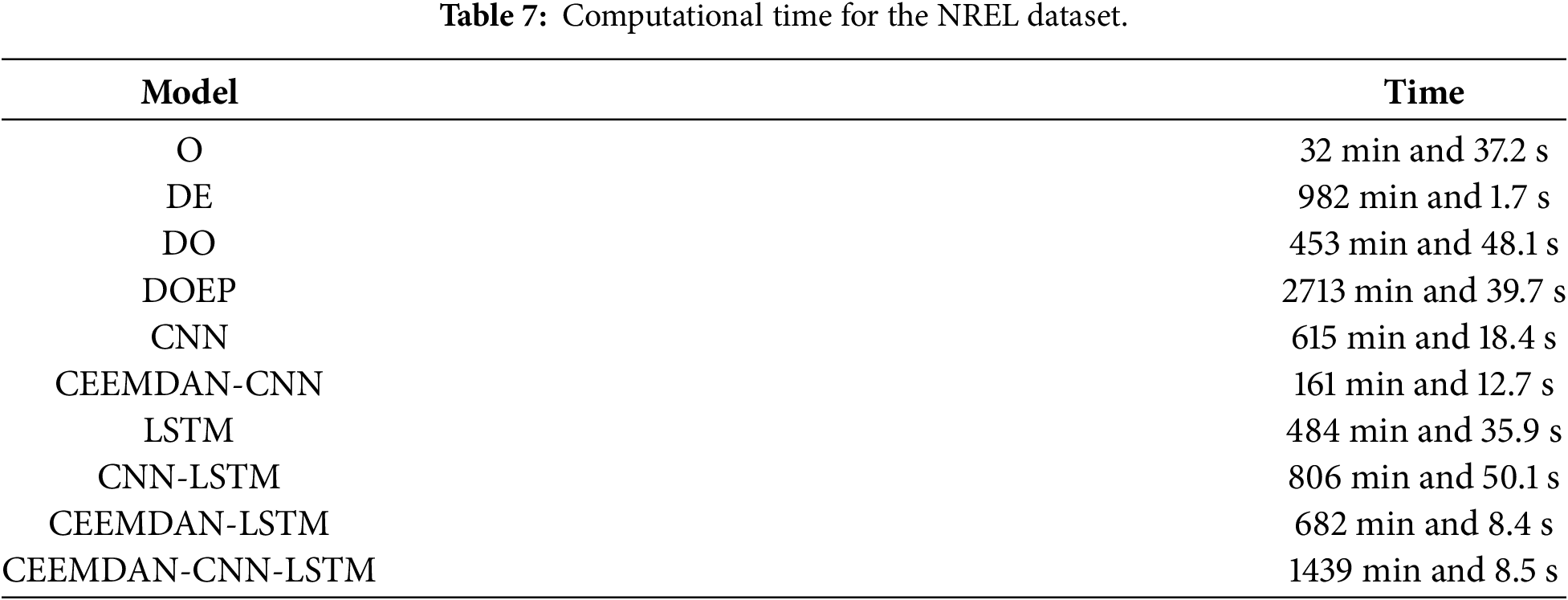
The proposed DOEP reduces the MSE by approximately 15%–60% for the ResPV-BDG dataset and 37%–92% in the NREL dataset. The DOEP framework delivers the strongest and most consistent performance compared to all benchmark methods across both datasets. The predicted-vs.-actual plots provide important evidence of prediction calibration: DOEP shows the best calibration, with points more tightly clustered along the trend line and a slope closer to 1. This improvement is also driven by the optimization strategy. The predictive model parameters are tuned using Segment-based EBQPSO, which enhances convergence speed and stability through structured information exchange among elite solutions via a segment-based transposon operator. This mechanism strengthens exploitation while preserving the diversity of solution, thereby reducing the risk of premature stagnation and sensitivity to the initial population. As a result, the optimized parameters tend to be more robust and stable. In addition to optimizing the predictive model parameters, Segment-based EBQPSO also optimizes the window size used to capture long-term dependencies in the data, although this may come at the cost of reduced precision in short-term fluctuation prediction. The residual boxplots further support the quantitative findings by illustrating the full error distribution, not only the average performance, and reflecting improved robustness against extreme errors. However, DOEP’s superior performance comes with a high computational cost compared with single-model pipelines that run much faster. This is a limitation of the proposed DOEP framework. Therefore, DOEP is most suitable for scenarios that prioritize accuracy and robustness, while simpler models may be preferable when computational speed is the primary constraint.

5  Conclusion

This study proposes a DOEP forecasting framework that integrates adaptive signal decomposition, the Segment-based EBQPSO parameter optimization, and residual error correction. Evaluations on two PV datasets demonstrate that the proposed DOEP framework consistently outperforms all benchmark models across both errorbased and goodness-of-fit metrics. Specifically, DOEP reduces mean square error by approximately 15%–60% on the ResPV-BDG dataset and 37%–92% on the NREL dataset, indicating strong generalization capability under both moderate and highly variable PV operating conditions.

Predicted-vs.-actual analyses further confirm the superior calibration of the proposed framework, with predictions more closely aligned to the ideal trend line and slopes approaching unity, reflecting improved scaling across the full output range. In addition, residual distribution analysis reveals a more compact error spread centered near zero, demonstrating enhanced robustness against extreme residual events compared with competing approaches. The observed performance improvements are primarily attributed to the Segment-based EBQPSO strategy, which enhances convergence stability through structured information exchange among elite solutions while maintaining population diversity. This design reduces sensitivity to initialization and mitigates the risk of premature convergence. Furthermore, joint optimization of the input window size enables more effective capture of long-term temporal dependencies, although short-term fluctuations may remain challenging during periods of extreme PV variability.

Despite its clear advantages in accuracy and stability, the DOEP framework incurs higher computational cost than single model pipelines, which may limit its applicability in resource constrained or real time environments. Future work will therefore focus on reducing computational complexity through parallel computing, surrogate assisted optimization, and lightweight decomposition strategies. Additional directions include adaptive windowing mechanisms and uncertainty-aware forecasting to better address short-term PV volatility. Finally, extensive validation across diverse climatic regions and PV system configurations will be conducted to further assess the robustness and practical applicability of the proposed framework in real-world grid operations.

Acknowledgement: The authors acknowledge the financial support from Intelligent Manufacturing Innovation Center, NTUST.

Funding Statement: The authors appreciate the financial support from the Ministry of Science and Technology of Taiwan (Contract Nos. 113-2221-E-011-130-MY2 and 113-2218-E-011-002) and the support from Intelligent Manufacturing Innovation Center (IMIC), National Taiwan University of Science and Technology (NTUST), Taipei, Taiwan.

Author Contributions: The authors confirm contribution to the paper as follows: Conceptualization, Desri Kristina Silalahi and Chao-Lung Yang; methodology, Desri Kristina Silalahi and Chao-Lung Yang; software, Desri Kristina Silalahi; validation, Yung-Yao Chen, Atinkut Atinafu Yilma and Chao-Lung Yang; data analysis, Desri Kristina Silalahi, Yung-Yao Chen, Atinkut Atinafu Yilma and Chao-Lung Yang; investigation, Yung-Yao Chen, Atinkut Atinafu Yilma and Chao-Lung Yang; writing—original draft preparation, Desri Kristina Silalahi and Chao-Lung Yang; writing—review and editing, Yung-Yao Chen, Atinkut Atinafu Yilma and Chao-Lung Yang; visualization, Desri Kristina Silalahi and Chao-Lung Yang; supervision, Yung-Yao Chen and Chao-Lung Yang; funding acquisition, Yung-Yao Chen. All authors reviewed and approved the final version of the manuscript.

Availability of Data and Materials: All data used in this study are from open-source datasets and can be accessed. These include the ResPV-BDG dataset [51] and the NREL dataset [52].

Ethics Approval: Not applicable.

Conflicts of Interest: The authors declare no conflicts of interest.

Abbreviations

References

1. Sharma V, Aziz SM, Haque MH, Kauschke T. Effects of high solar photovoltaic penetration on distribution feeders and the economic impact. Renew Sustain Energy Rev. 2020;131:110021. doi:10.1016/j.rser.2020.110021. [Google Scholar] [CrossRef]

2. Gaboitaolelwe J, Zungeru AM, Yahya A, Lebekwe CK, Vinod DN, Salau AO. Machine learning based solar photovoltaic power forecasting: a review and comparison. IEEE Access. 2023;11:40820–45. doi:10.1109/ACCESS.2023.3270041. [Google Scholar] [CrossRef]

3. Dou X, Cui Z. Neural network-based forecasting and uncertainty analysis of new power generation capacity of electric energy. Energy Inform. 2025;8(1):85. doi:10.1186/s42162-025-00546-0. [Google Scholar] [CrossRef]

4. Piantadosi G, Dutto S, Galli A, De Vito S, Sansone C, Di Francia G. Photovoltaic power forecasting: a Transformer based framework. Energy AI. 2024;18:100444. doi:10.1016/j.egyai.2024.100444. [Google Scholar] [CrossRef]

5. Tajjour S, Chandel SS, Malik H, Márquez FPG, Alotaibi MA. Daily power generation forecasting for a grid-connected solar power plant using transfer learning technique. Appl Intell. 2025;55(6):383. doi:10.1007/s10489-024-06090-w. [Google Scholar] [CrossRef]

6. Geetha A, Usha S, Santhakumar J, Salkuti SR. Analysis of dust accumulation effects on the long-term performance of solar PV panels. AIMS Energy. 2025;13(3):493–516. doi:10.3934/energy.2025019. [Google Scholar] [CrossRef]

7. Shen Y, Fouladirad M, Grall A. Impact of dust and temperature on photovoltaic panel performance: a model-based approach to determine optimal cleaning frequency. Heliyon. 2024;10(16):e35390. doi:10.1016/j.heliyon.2024.e35390. [Google Scholar] [PubMed] [CrossRef]

8. Abouzeid AF, Eleraky H, Kalas A, Rizk R, Elsakka MM, Refaat A. Experimental validation of a low-cost maximum power point tracking technique based on artificial neural network for photovoltaic systems. Sci Rep. 2024;14(1):18280. doi:10.1038/s41598-024-67306-0. [Google Scholar] [PubMed] [CrossRef]

9. Marangis D, Tziolis G, Livera A, Makrides G, Kyprianou A, Georghiou GE. Intelligent maintenance approaches for improving photovoltaic system performance and reliability. Sol RRL. 2025;9(16):2500289. doi:10.1002/solr.202500289. [Google Scholar] [CrossRef]

10. Miao Y, Lau SSY, Lo KKN, Song Y, Lai H, Zhang J, et al. Harnessing climate variables for predicting PV power output: a backpropagation neural network analysis in a subtropical climate region. Sol Energy. 2023;264(1):111979. doi:10.1016/j.solener.2023.111979. [Google Scholar] [CrossRef]

11. Korkmaz D. SolarNet: a hybrid reliable model based on convolutional neural network and variational mode decomposition for hourly photovoltaic power forecasting. Appl Energy. 2021;300:117410. doi:10.1016/j.apenergy.2021.117410. [Google Scholar] [CrossRef]

12. Ferkous K, Guermoui M, Bellaour A, boulmaiz T, Bailek N. Enhancing photovoltaic energy forecasting: a progressive approach using wavelet packet decomposition. Clean Energy. 2024;8(3):95–108. doi:10.1093/ce/zkae027. [Google Scholar] [CrossRef]

13. Zhai C, He X, Cao Z, Abdou-Tankari M, Wang Y, Zhang M. Photovoltaic power forecasting based on VMD-SSA-Transformer: multidimensional analysis of dataset length, weather mutation and forecast accuracy. Energy. 2025;324(9):135971. doi:10.1016/j.energy.2025.135971. [Google Scholar] [CrossRef]

14. RajasundrapandiyanLeebanon T, Murugan NSS, Kumaresan K, Jeyabose A. Long-term solar radiation forecasting in India using EMD, EEMD, and advanced machine learning algorithms. Environ Monit Assess. 2025;197(3):310. doi:10.1007/s10661-025-13738-8. [Google Scholar] [PubMed] [CrossRef]

15. Liang J, Yin L, Xin Y, Li S, Zhao Y, Song T. Short-term photovoltaic power prediction based on CEEMDAN-PE and BiLSTM neural network. Electr Power Syst Res. 2025;246:111706. doi:10.1016/j.epsr.2025.111706. [Google Scholar] [CrossRef]

16. Jaseena KU, Kovoor BC. Decomposition-based hybrid wind speed forecasting model using deep bidirectional LSTM networks. Energy Convers Manag. 2021;234:113944. doi:10.1016/j.enconman.2021.113944. [Google Scholar] [CrossRef]

17. Atique S, Noureen S, Roy V, Bayne S, Macfie J. Time series forecasting of total daily solar energy generation: a comparative analysis between ARIMA and machine learning techniques. In: 2020 IEEE Green Technologies Conference (GreenTech). Piscataway, NJ, USA: IEEE; 2020. p. 175–80. doi:10.1109/GreenTech46478.2020.9289796. [Google Scholar] [CrossRef]

18. Markovics D, Mayer MJ. Comparison of machine learning methods for photovoltaic power forecasting based on numerical weather prediction. Renew Sustain Energy Rev. 2022;161:112364. doi:10.1016/j.rser.2022.112364. [Google Scholar] [CrossRef]

19. Etxegarai G, Zapirain I, Camblong H, Ugartemendia J, Hernandez J, Curea O. Photovoltaic energy production forecasting in a short term horizon: comparison between analytical and machine learning models. Appl Sci. 2022;12(23):12171. doi:10.3390/app122312171. [Google Scholar] [CrossRef]

20. Marzouglal M, Souahlia A, Bessissa L, Mahi D, Rabehi A, Alharthi YZ, et al. Prediction of power conversion efficiency parameter of inverted organic solar cells using artificial intelligence techniques. Sci Rep. 2024;14(1):25931. doi:10.1038/s41598-024-77112-3. [Google Scholar] [PubMed] [CrossRef]

21. Ağır TT. Estimation of daily photovoltaic power one day ahead with hybrid deep learning and machine learning models. Energy Sci Eng. 2025;13(4):1478–91. doi:10.1002/ese3.1994. [Google Scholar] [CrossRef]

22. Ouyang Z, Li Z, Chen X. Day-ahead photovoltaic power forecasting with multi-source temporal-feature convolutional networks. Energy Inform. 2025;8(1):68. doi:10.1186/s42162-025-00531-7. [Google Scholar] [CrossRef]

23. Liu X, Dong X, Zhang L, Chen J, Wang C. Least squares support vector regression for complex censored data. Artif Intell Med. 2023;136(1):102497. doi:10.1016/j.artmed.2023.102497. [Google Scholar] [PubMed] [CrossRef]

24. Van Craen A, Breyer M, Pflüger D. PLSSVM: a (multi-)GPGPU-accelerated least squares support vector machine. In: 2022 IEEE International Parallel and Distributed Processing Symposium Workshops (IPDPSW). Piscataway, NJ, USA: IEEE; 2022. p. 818–27. doi:10.1109/ipdpsw55747.2022.00138. [Google Scholar] [CrossRef]

25. Essam Y, Ahmed AN, Ramli R, Chau K-W, Idris Ibrahim MS, Sherif M, et al. Investigating photovoltaic solar power output forecasting using machine learning algorithms. Eng Appl Comput Fluid Mech. 2022;16(1):2002–34. doi:10.1080/19942060.2022.2126528. [Google Scholar] [CrossRef]

26. Al-Ali EM, Hajji Y, Said Y, Hleili M, Alanzi AM, Laatar AH, et al. Solar energy production forecasting based on a hybrid CNN-LSTM-transformer model. Mathematics. 2023;11(3):676. doi:10.3390/math11030676. [Google Scholar] [CrossRef]

27. Wang K, Qi X, Liu H. Photovoltaic power forecasting based LSTM-Convolutional Network. Energy. 2019;189(4):116225. doi:10.1016/j.energy.2019.116225. [Google Scholar] [CrossRef]

28. Jiang J, Hu S, Xu L, Wang T. Short-term PV power prediction based on VMD-CNN-IPSO-LSSVM hybrid model. Int J Low-Carbon Technol. 2024;19:1160–7. doi:10.1093/ijlct/ctae060. [Google Scholar] [CrossRef]

29. Gu B, Shen H, Lei X, Hu H, Liu X. Forecasting and uncertainty analysis of day-ahead photovoltaic power using a novel forecasting method. Appl Energy. 2021;299:117291. doi:10.1016/j.apenergy.2021.117291. [Google Scholar] [CrossRef]

30. Yang M, Peng T, Su X, Ma M. Short-term photovoltaic power interval prediction based on the improved generalized error mixture distribution and wavelet packet-LSSVM. Front Energy Res. 2021;9:757385. doi:10.3389/fenrg.2021.757385. [Google Scholar] [CrossRef]

31. Pérez-Rodríguez SA, Álvarez-Alvarado JM, Romero-González JA, Aviles M, Mendoza-Rojas AE, Fuentes-Silva C, et al. Metaheuristic algorithms for solar radiation prediction: a systematic analysis. IEEE Access. 2024;12(3):100134–51. doi:10.1109/ACCESS.2024.3429073. [Google Scholar] [CrossRef]

32. Coronado-Mendoza A, Camas-Náfate M, Artal-Sevil JS, Domínguez-Navarro JA. Optimum design of a photovoltaic inverter system based on GA, PSO and GWO algorithms with a MPPT sliding mode control. Energies. 2025;18(8):1911. doi:10.3390/en18081911. [Google Scholar] [CrossRef]

33. Zhang ZS. Quantum-behaved particle swarm optimization algorithm for economic load dispatch of power system. Expert Syst Appl. 2010;37(2):1800–3. doi:10.1016/j.eswa.2009.07.042. [Google Scholar] [CrossRef]

34. Zheng M, Bu Q, Yi W, Ye Z. Short-term photovoltaic power prediction for microgrids based on FCM-QPSO–LSTM. Int J High Speed Electron Syst. 2025;34(4):2540361. doi:10.1142/S0129156425403614. [Google Scholar] [CrossRef]

35. Li G, Wei X, Yang H. Decomposition integration and error correction method for photovoltaic power forecasting. Measurement. 2023;208(5):112462. doi:10.1016/j.measurement.2023.112462. [Google Scholar] [CrossRef]

36. Zhang L, Liu L, Chen W, Lin Z, He D, Chen J. Photovoltaic power generation forecasting based on secondary data decomposition and hybrid deep learning model. Energies. 2025;18(12):3136. doi:10.3390/en18123136. [Google Scholar] [CrossRef]

37. Sun N, Zhang N, Zhang S, Peng T, Jiang W, Ji J, et al. An integrated framework based on an improved Gaussian process regression and decomposition technique for hourly solar radiation forecasting. Sustainability. 2022;14(22):15298. doi:10.3390/su142215298. [Google Scholar] [CrossRef]

38. Feng D, Zhang H, Wang Z. Hourly photovoltaic power prediction based on signal decomposition and deep learning. J Phys Conf Ser. 2024;2728(1):012011. doi:10.1088/1742-6596/2728/1/012011. [Google Scholar] [CrossRef]

39. Zhang R, Xu Z, Liu S, Fu K, Zhang J. Prediction of ultra-short-term photovoltaic power using BiLSTM-Informer based on secondary decomposition. Energies. 2025;18(6):1485. doi:10.3390/en18061485. [Google Scholar] [CrossRef]

40. Guermoui M, Fezzani A, Mohamed Z, Rabehi A, Ferkous K, Bailek N, et al. An analysis of case studies for advancing photovoltaic power forecasting through multi-scale fusion techniques. Sci Rep. 2024;14(1):6653. doi:10.1038/s41598-024-57398-z. [Google Scholar] [PubMed] [CrossRef]

41. Yang L, Gao Y, Cui X. Research on PV power prediction model based on data dimensionality reduction and optimization of CEEMDAN-SSA-GRU algorithm. J Renew Sustain Energy. 2025;17(4):043509. doi:10.1063/5.0276964. [Google Scholar] [CrossRef]

42. Xu W, Li D, Dai W, Wu Q. Informer short-term PV power prediction based on sparrow search algorithm optimised variational mode decomposition. Energies. 2024;17(12):2984. doi:10.3390/en17122984. [Google Scholar] [CrossRef]

43. Li JN, Tian MZ, Zhao WH, He XM, Zhang H, ZHou HJ. A data-driven method for forecasting the photovoltaic substation active power. In: 2024 4th Power System and Green Energy Conference (PSGEC). Piscataway, NJ, USA: IEEE; 2024. p. 668–72. doi:10.1109/PSGEC62376.2024.10721142. [Google Scholar] [CrossRef]

44. Zhou Y, Zhou N, Gong L, Jiang M. Prediction of photovoltaic power output based on similar day analysis, genetic algorithm and extreme learning machine. Energy. 2020;204:117894. doi:10.1016/j.energy.2020.117894. [Google Scholar] [CrossRef]

45. Thu NTH, Bao PQ, Nam NVN. Multiple step ahead forecasting of rooftop solar power based on a novel hybrid model of CEEMDAN-bidirectional LSTM network with structure optimized by PSO method. In: 2022 11th International Conference on Control, Automation and Information Sciences (ICCAIS). Piscataway, NJ, USA: IEEE; 2022. p. 522–8. doi:10.1109/ICCAIS56082.2022.9990323. [Google Scholar] [CrossRef]

46. Abbas BK, Jabbar QA, Hameed RT. Optimizing benchmark functions using particle swarm optimization (PSO). Al-Salam J Eng Technol. 2025;4(1):192–8. doi:10.55145/ajest.2025.04.01.019. [Google Scholar] [CrossRef]

47. Fang W, Sun J, Ding Y, Wu X, Xu W. A review of quantum-behaved particle swarm optimization. IETE Tech Rev. 2010;27(4):336–48. doi:10.4103/0256-4602.64601. [Google Scholar] [CrossRef]

48. Yang ZL, Wu A, Min HQ. An improved quantum-behaved particle swarm optimization algorithm with elitist breeding for unconstrained optimization. Comput Intell Neurosci. 2015;2015(1):1–12. doi:10.1155/2015/326431. [Google Scholar] [PubMed] [CrossRef]

49. Zhang R, Li G, Bu S, Kuang G, He W, Zhu Y, et al. A hybrid deep learning model with error correction for photovoltaic power forecasting. Front Energy Res. 2022;10:948308. doi:10.3389/fenrg.2022.948308. [Google Scholar] [CrossRef]

50. Zhong C, Lai CS, Ng W, Tao Y, Wang T, Lai LL. Multi-view deep forecasting for hourly solar irradiance with error correction. Solar Energy. 2021;228(7):308–16. doi:10.1016/j.solener.2021.09.043. [Google Scholar] [CrossRef]

51. ResPV-BDG Dataset. 2025 [cited 2025 Dec 23]. Available from: https://www.kaggle.com/datasets/educatelabs/power-output-photovoltaic/data. [Google Scholar]

52. NREL solar power data for integration studies. [cited 2025 Dec 23]. Available from: https://www.nrel.gov/grid/solar-power-data. [Google Scholar]

53. Zhao S, Yang X, Li K, Li X, Qi W, Huang X. Photovoltaic output prediction based on VMD disturbance feature extraction and WaveNet. Front Energy Res. 2024;12:1422728. doi:10.3389/fenrg.2024.1422728. [Google Scholar] [CrossRef]

54. Bu Q, Ye Z, Zhuang S, Luo F, Yue F. Research on short-term prediction of photovoltaic power via improved VMD-based dynamic model fusion and adaptive boundary optimization. Sustain Energy Res. 2025;12(1):51. doi:10.1186/s40807-025-00201-y. [Google Scholar] [CrossRef]