An Agentic Artificial Intelligence Observer for Predictive Maintenance in Electrolysers

1  Introduction

Electrolysers can convert electrical energy obtained from renewable energy sources into low-emission hydrogen [1]. One of the major constraints to ramping up the market share of hydrogen production technology is the operation and maintenance costs of electrolyser plants [2]. A poorly maintained electrolyser will lead to operational failures, safety risks, reduced efficiency, and consequently, increased hydrogen costs. Monitoring systems such as intelligent observers can provide useful information for electrolyser maintenance. They use sensor signals connected to programmable logic controllers (PLC) to obtain information from the plant and allow for monitoring and fault detection in the electrolyser. This is demonstrated in scientific literature [3–5].

The monitoring system can be equipped with predictive maintenance models, which rely on accurate sensor measurements to enable the prediction of potential abnormalities [6–8]. However, if the sensor fails, there will be an incorrect prediction of abnormalities [9]. This can result in wrong maintenance, and consequently potential damage in the electrolyser, which is made up of the stack and the balance of plant (BoP). In a paper by da Silva et al. [10], the authors indicated that sensors are often the weak link in many engineering applications since they are less reliable than the system they are observing. Among the different sensor faults, those due to drifts are probably the most difficult to detect because the loss of accuracy in measurements can be slow but progressive over time [11]. Another drawback with existing predictive models is that they require enormous training data, which is not available at the early stage of plant operation [7]. In this paper, the authors develop an artificial intelligence (AI)-based observer for detecting faults in sensors, without the use of enormous sensor data, Fig. 1. Fuzzy logic [12] is used to detect faulty sensor readings due to abnormal drift behaviour, while a long short-term memory (LSTM) network complements the fuzzy system to provide correct sensor data.

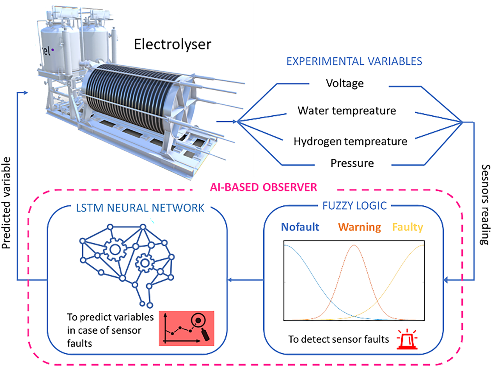
Figure 1: Graphical abstract of paper with focus on an AI-based observer

Regarding previous scientific literature, there are very few papers that have developed AI-based solutions for the detection of sensor faults in electrolysis plants.

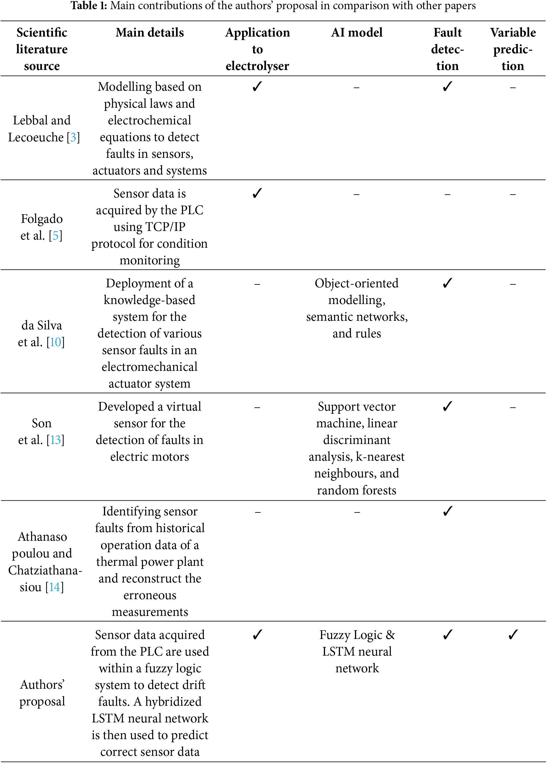
In this sense, Lebbal and Lecoeuche [3] developed an offline algorithm to detect and isolate faults on actuators and sensors in an electrolyser. Folgado et al. [5] developed a condition monitoring system based on sensor data acquired from the PLC of an electrolyser. In a paper by da Silva et al. [10], the authors deployed a knowledge-based system using tools such as object-oriented modelling, semantic networks, and rules to detect various sensor faults in an electromechanical actuator system. In another paper by Son et al. [13], the authors developed a virtual sensor for the detection of faults in electric motors. The sensor acquires three types of signals involving vibration, current, and flux from the induction motors and then uses models such as support vector machine, linear discriminant analysis, k-nearest neighbours, and random forests to classify the faults. Athanasopoulou and Chatziathanasiou [14] describe a procedure for identifying sensor faults from historical operation data of a thermal power plant and reconstructing the erroneous measurements using a data mining algorithm.

Based on the above, the main contribution of this paper is the development of an AI-based observer that combines fuzzy logic and a long short-term memory (LSTM) network to detect abnormalities in electrolyser sensor signals and predict them in case of failure. The fuzzy system provides an immediate, model-based solution for fault detection from the moment the plant is commissioned, while a long-short-term memory (LSTM) network [15] offers a data-driven solution for signal prediction once enough normal operating data has been collected. This overall contribution is summarised in Table 1.

The system developed by the authors follows the transparent (white-box) branch of explainable AI [16] in the sense that ours is a rule-based fuzzy-logic model that is hybridized with a neural network. The inclusion of fuzzy logic ensures that the model is auditable by design. In parallel, a recent wave of neuro-symbolic and white-box neural approaches aims to embed interpretability into model structure rather than explain it afterwards. For example, the Deep Expert Network (DEN) [17] for fault diagnosis builds end-to-end models from learnable signal-processing, statistical, and logical operators to yield a fully traceable decision route. We position our contribution as a pragmatic, readily deployable point on this spectrum—preserving full transparency and low integration cost on real assets, while being complementary to learnable-operator networks when data and training are limited. To address the authors’ proposal, the paper is organised as follows: Section 2 does a classification of sensor faults that can appear in an electrolyser, identifying the challenges to detect some types of sensor faults. Section 3 describes the materials and methods needed to develop both the fuzzy system and the LSTM neural network as well as the physical connection in the real plant. Finally, Sections 4 and 5 discuss experimental results and conclusions, respectively.

2  Challenges of Maintaining a Healthy Electrolysis Plant

During electrolyser operation, various failures can occur that can cause the stack to transition from a healthy to a damaged state. Some of these faults are due to abnormal operating conditions, improper manufacturing processes or inadequate maintenance. To address some of these problems, modern electrolysers have sensors embedded within their control system to detect sub-optimal operating conditions, which can damage the stack. The introduction of these sensors further enables deployment of advanced maintenance techniques such as predictive maintenance to forecast potential problems [4–7]. But, despite advancements in maintenance, problems can still occur within an electrolyser: either with the embedded sensors or the internal stack components such as the membrane, bipolar plates, etc. We therefore present the global possibilities of these fault scenarios, as shown in Table 2.

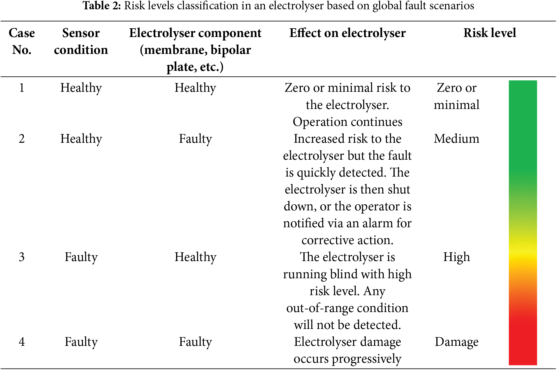
Based on Table 2, case 1 is the preferred option, which has zero or minimal risk to the electrolyser. However, over the lifetime of the electrolyser, operating conditions such as contaminated feed water, high temperature, pressure, current density, or voltage can change, and this places the electrolyser in case 2. Fortunately, the embedded sensors can quickly detect any such abnormalities within a few seconds to minutes, and either shut down the electrolyser or alert the operator to perform corrective action. In most scenarios, the electrolyser can operate for an extended period if it occasionally operates between cases 1 and 2. Case 3 often occurs because the sensors themselves can also develop faults. When this occurs, the control system is said to be operating blind. In such cases, the risk of failure is very high because a sudden occurrence of a sub-optimal condition will not be detected, and failure of an internal component will occur. The authors’ proposal focuses on case 3 with the aim of detecting when a sensor has failed due to a drift fault. An undetected sensor failure is often a strong precursor to case 4, which causes electrolyser damage. The system developed by the authors avoids case 4, which means that if cases 3 and 2 are resolved, the risk level is minimal or medium (green to yellow).

Regarding scientific literature, there are limited papers concerning this topic so this paper will contribute to the advancement of knowledge in this area. The next sub-sections discuss further some of the internal faults in the electrolyser as well as those relating to their embedded sensors.

2.1 Problems with the Stack Components of Electrolysers

Commercial electrolysis technology can be classified into low-to-medium temperature (alkaline electrolysers and proton exchange membrane electrolysers) and high-temperature electrolysis (solid oxide electrolysers). In this case, the authors will carry out the experimentation with a PEM electrolyser. The main stack components of a PEM electrolyser include the membrane, catalyst layer (CL), porous transport layer (PTL), bipolar plates (BPP), seals and gasket [18]. The membrane is sandwiched between two catalyst layers (∼1–10 µm) which serve as the electrodes of the cell, typically consisting of an iridium-based catalyst for the anode and a platinum-based catalyst for the cathode. The catalyst facilitates the reaction that splits water molecules into hydrogen and hydroxide ions. Outside each catalyst layer are diffusion layers: The gas diffusion layer (GDL, ∼100–300 µm) on the cathode side and the porous transport layer (PTL, ∼250–500 µm) on the anode side. The GDL is primarily responsible for gaseous transport (hydrogen gas out), while the PTL is responsible for liquid and gaseous transport (liquid water in; oxygen gas out). The BPP contains flow fields to distribute reactants (water) and remove products (oxygen and hydrogen gas). The seals and gaskets mainly keep the fluids and gases in their respective sections. Various faults can occur with any of these components. This is illustrated in Fig. 2 with possible causes included.

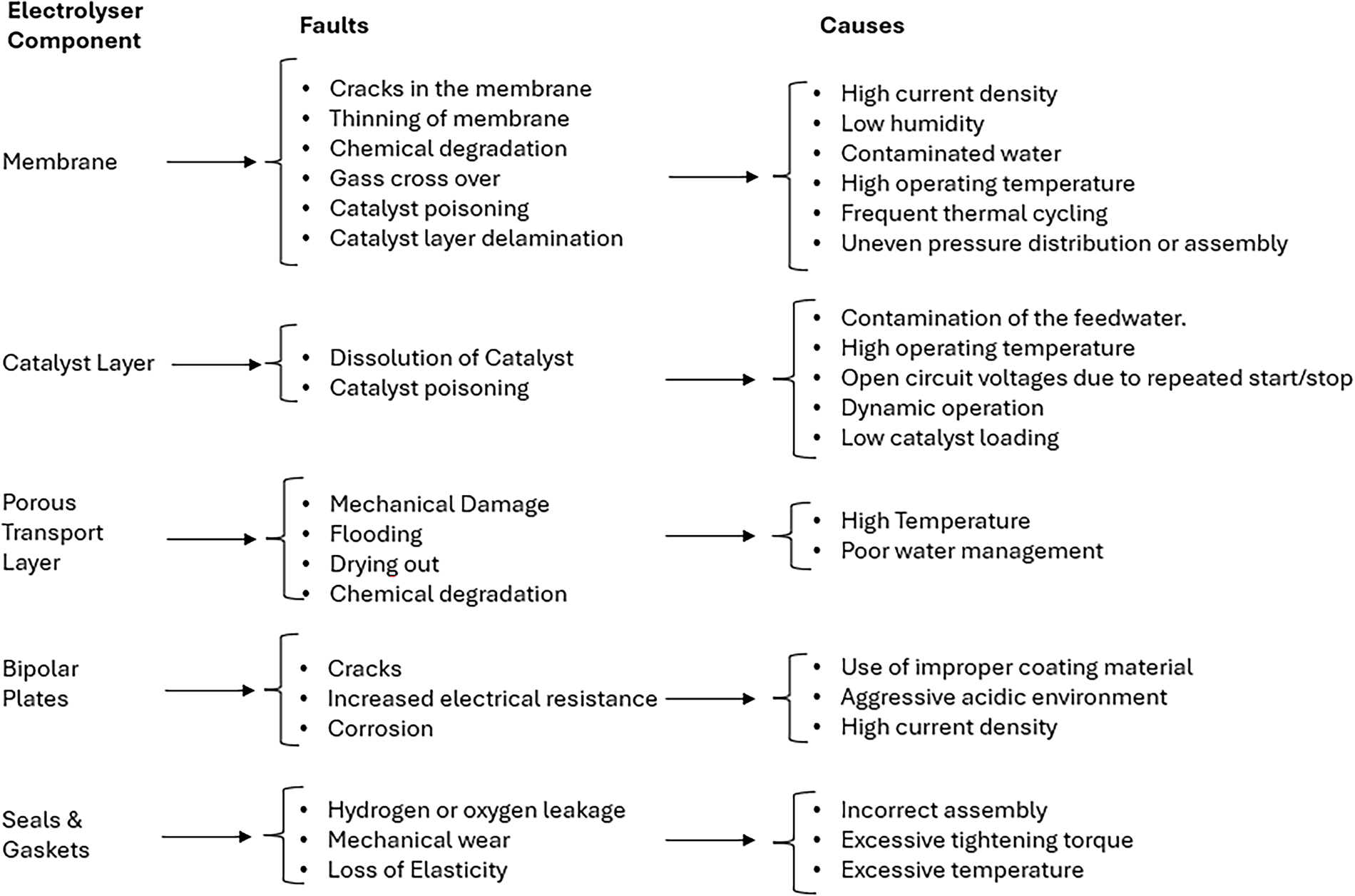
Figure 2: Analysis of faults in an electrolyser

2.2 Problems with Sensors Used in Electrolysers

Scientific literature has indicated the use of sensors for predictive maintenance in electrolysers [3,5]. Sensors are connected to PLCs, which control various subsystems within the electrolyser, and can also log sensor measurements to a local or remote database. PLCs are among the most used controller devices in electrolysers [19]. The sensor signals are processed using PLC ladder logic and result in the activation of output signals to energize devices such as valves, relays, lamps, and others. If the sensor fails, erroneous control actions will occur. Various types of sensor faults exist, as shown in Fig. 3 [10]. Severe or hard failures are those in which a sudden loss of signal happens, such as a wire break (Fig. 3b). There can also be fluctuating signals referred to as spikes or noise (Fig. 3c) which can be due to vibrations or sudden changes in the process being measured. Another type of sensor fault is called drift (Fig. 3d), in which the value being read gradually increases or decreases gradually over time.

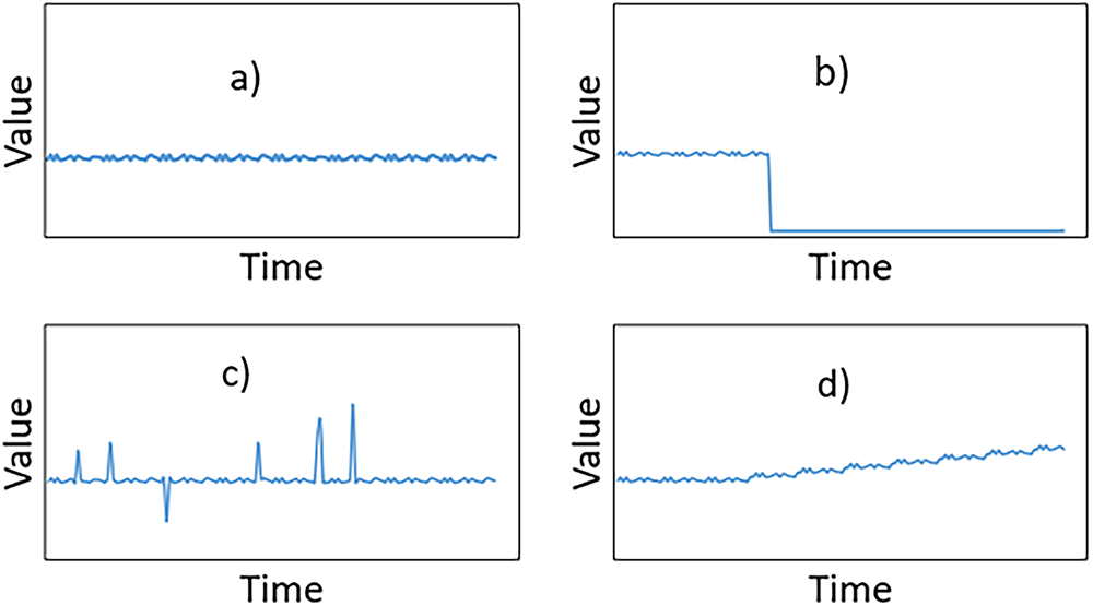
Figure 3: Various types of sensor faults. (a) Normal. (b) Hard. (c) Spikes. (d) Drift

From the various sensor faults, drift faults are among the most difficult to detect since they can have a progressive but slow evolution [10]. In these cases, AI-based techniques, such as LSTM, can be useful for predicting faulty sensor readings due to drift, but they often require large amounts of training data that are not available in the early stages of plant operation [11].

In this paper, the authors address the challenge of problems with sensors rather than stack components. Sensors are part of the BoP, and the correct stack operation depends on their monitoring. For this purpose, the authors have developed an AI-based observer comprising a fuzzy system and an LSTM neural network to solve drift faults in a sensor connected to an electrolyser even without existing fault or training data.

3  Materials and Methods

The materials needed to carry out the solution developed in this work are the following:

•   1 Nm3/h H2-proton exchange membrane (PEM) electrolyser, available in the research centre CITES at the University of Huelva, Fig. 4.

•   A detail of a section of the piping diagram of the PEM electrolyser, Fig. 5. The authors addressed the design, implementation, and control of the balance of plant (BoP) in a previous work [19].

•   PLC 1500 Siemens® hardware and 24 V direct current (DC) power supply.

•   Siemens® software: Totally Integrated Automation (TIA) portal v15.1.

•   MATLAB® software version R2022b.

•   A computer equipped with Intel® Core i7-7700HQ CPU @2.8 GHz; 16 GB memory, 64-bit, x64-based processor, Windows® 7 Operating System.

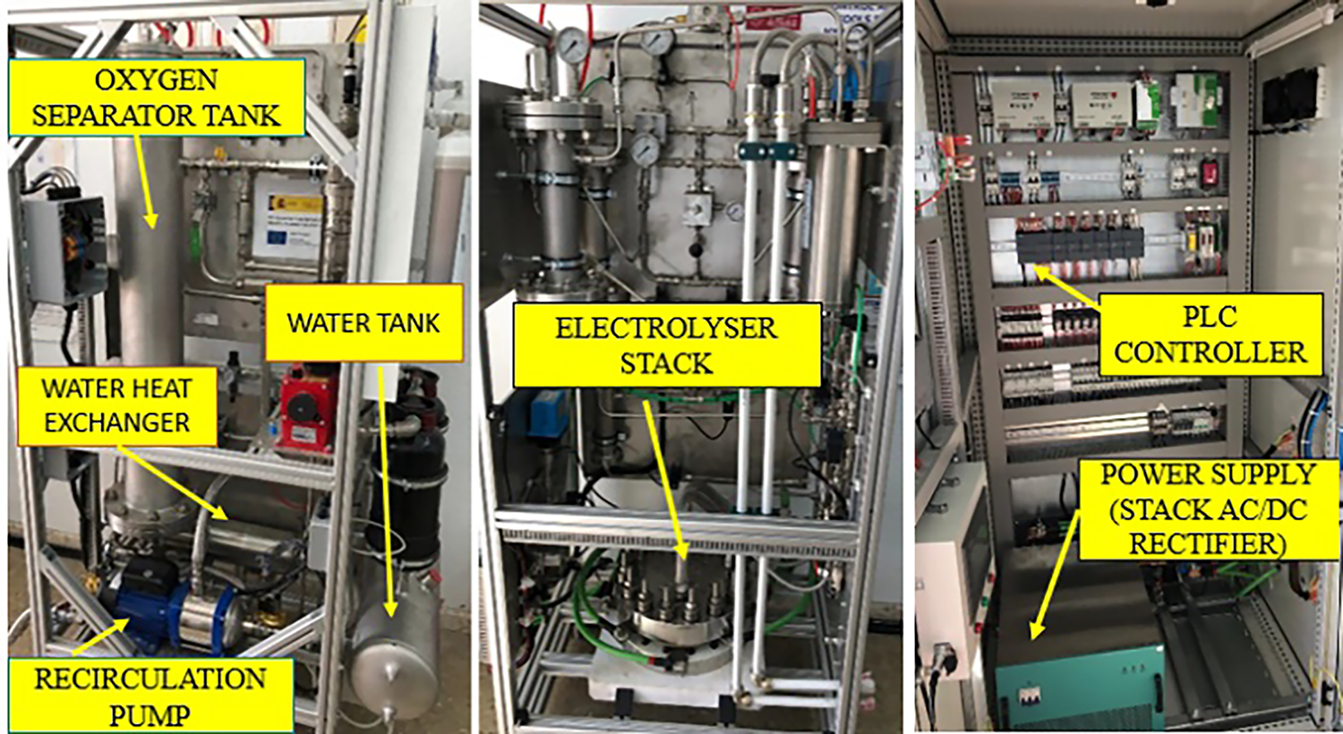
Figure 4: Layout of PEM electrolyser plant used in the research

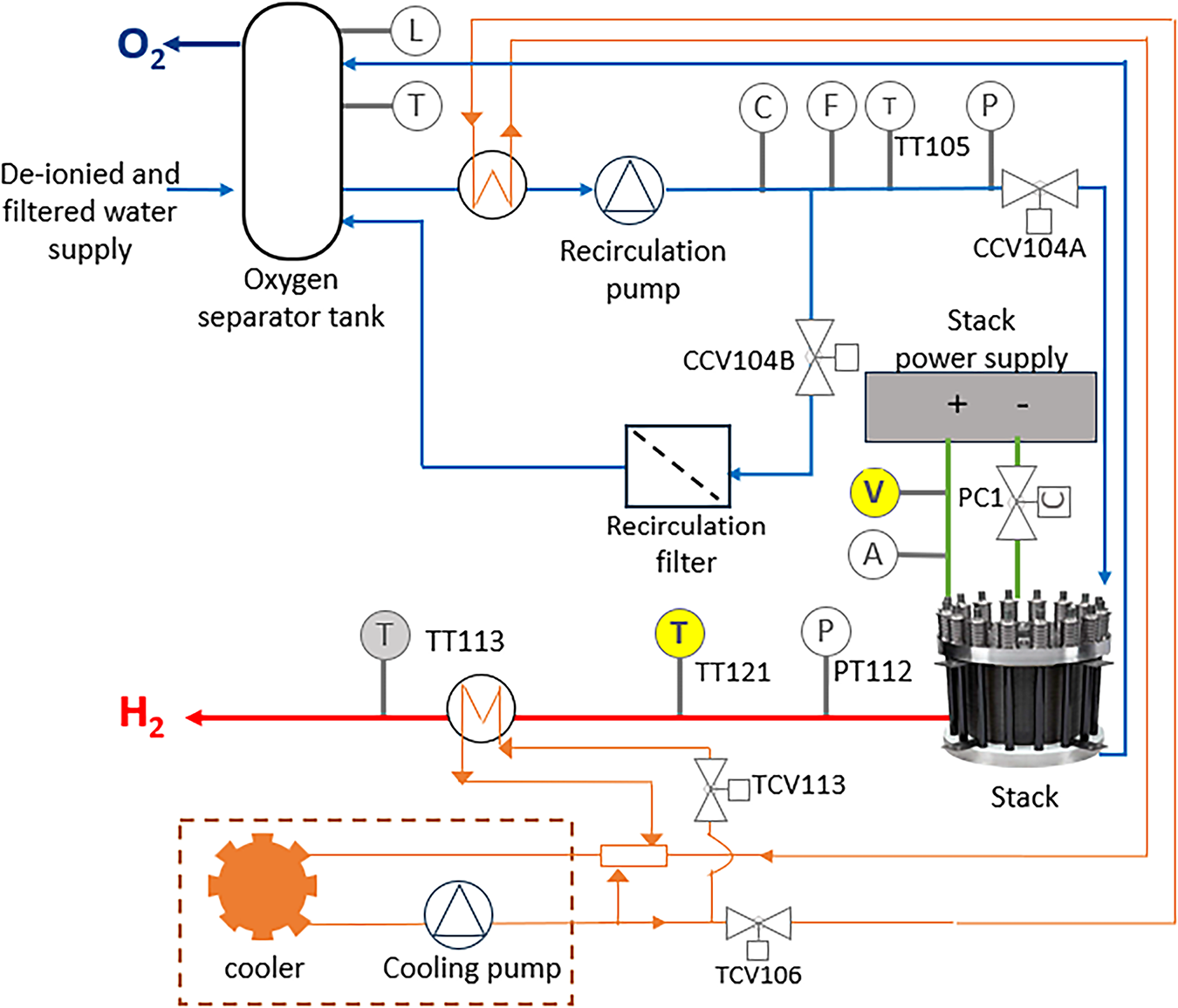
Figure 5: A section of the balance of plant (BoP) of the electrolyser

The methodology, defined by the authors to develop the AI-based observer for detecting and predicting drift-type sensor faults in an electrolyser, is described below. It is applied to a real case, a 1 Nm3/h H2-PEM electrolyser, but it can be extended to any other electrolyser model. To demonstrate the feasibility of the authors’ proposed method, the hydrogen temperature sensor, TT121 (see Fig. 5), has been chosen for this research because it is a critical variable in the hydrogen production process [20]. The effect of temperature on the degradation of membranes (a component of the stack, the interface where the separation between oxygen and hydrogen occurs) has been investigated by Chandesris et al. [21]. The authors confirmed that degradation mainly occurs at the cathode side where hydrogen gas is produced. If the hydrogen temperature sensor TT121 fails or gives an incorrect measurement, the cell membrane will be degraded, causing loss of efficiency and unsafe operation.

To detect drift faults in the TT121 hydrogen temperature sensor, authors propose to find a correlation between hydrogen temperature and stack efficiency. This intuition in approaching the problem is not accidental, since it is logical to think that the more heat is dissipated (more electrical power consumption) the less efficient the stack will be.

3.1 Theoretical Analysis of the Problem Addressed

To establish the relationship between efficiency and temperature, expression (1) is considered [22]. This equation relates the heat dissipated to the electrical power consumed by the electrolytic cell. To scale up from a single cell to a multi-cell stack, expression (2) can be obtained.

ηcell=1−QcellPcell(1)

ηstack=1−QstackPstack=1−NcellQcellNcellPcell(2)

where:

ηcell is the cell efficiency

Qcell is the heat dissipated in the cell (W)

Pcell is the electrical power consumed by the cell (W)

ηstack is the stack efficiency

Qstack is the heat dissipated in the stack (W)

Pstack is the electrical power consumed by the stack (W)

Ncell is the number of cells in the stack

From the physicochemical point of view, the heat dissipated in the stack, Qstack, can be expressed in terms of the heat due to the hydrogen, oxygen, and water flows in the electrolytic reaction (3).

Qstack=(m˙H2cH2+m˙O2cO2+m˙H2OcH2O)ΔT(3)

where:

m˙H2 is the stack hydrogen mass flow (g/s)

cH2 is the specific heat capacity of hydrogen (14.30 J/g K)

m˙O2is the stack oxygen mass flow (g/s)

cO2 is the specific heat capacity of oxygen (0.92 J/g K)

m˙H2O is the water mass flow (g/s)

cH2O is the specific heat capacity of water (4.18 J/g K)

ΔT is the change in temperature from initial to new state (K)

The hydrogen m˙H2, oxygen m˙O2 and water m˙H2O mass flows can be obtained from (4).

m˙i=mol˙iMi(4)

where:

i is H2, O2 or H2O, respectively

mol˙H2 is the stack hydrogen molar flow (mol/s)

MH2 is the hydrogen molar mass (2 g/mol)

mol˙O2 is the stack oxygen molar flow (mol/s); in electrolysis, molar relation between H2, and O2 is: mol˙O2=mol˙H22

MO2 is the oxygen molar mass (32 g/mol)

mol˙H2O is the water molar flow (mol/s)

MH2O is the water molar mass (18 g/mol)

From (3),(4) can be written as (5).

Qstack=(mol˙H2MH2cH2+mol˙O2MO2cO2+mol˙H2OMH2OcH2O)ΔT(5)

Regarding the molar flow, according to Faraday’s law, the hydrogen molar flow of an electrolytic stack, powered by an electrical current Istack, can be obtained from (6):

mol˙H2=NcellIstack2F(6)

where:

Istack is the current consumed by the stack (A)

F is the Faraday Constant (96 485.33 As/mol)

On the other hand, the electrical power consumed by the stack can be written as (7).

Pstack=IstackVstack(7)

where:

Vstack is the voltage required by the stack (V).

Then, replacing (3), (5), (6) and (7) in (2), it is possible to obtain (8), which relates temperature and stack efficiency:

ΔT=(1−ηstack(MH2cH2+12MO2cO2)2F+m˙H2OcH2OPstack)(8)

Eq. (8) shows that the greater the temperature change, the worse the efficiency. Therefore, when the temperature change is maximum, ΔTmax, the stack operates at minimum efficiency, ηstack,min. Consequently, maximum efficiency, ηstack,max, will correspond to minimum temperature change, ΔTmin.

Once the expression that relates temperature change and efficiency has been obtained, we consider developments from Bessarabov and Millet [23] to obtain the expression that allows to measure the efficiency (9) for a single-cell and (10) for a multi-cell stack.

ηcell=VthVcell(9)

ηstack=VthstackVstack=NcellVthNcellVcell(10)

where:

Vth is the theoretical potential of the reversible redox reaction in the water decomposition (1.23 V),

Vcell is the experimental cell voltage (V).

Then, expression (10) allows us to calculate stack efficiency at any operation point, and expression (8) computes the temperature change, taking into account the calculated value of the efficiency.

3.2 Development of the Fuzzy System

Health indicators within a process can be used as inputs to develop a fuzzy system that outputs diagnostic signals. In a related work, Mazzoleni et al. [24] developed a model based on fuzzy inference for a steel making plant to classify fault conditions into healthy (no fault), warning, and faulty. In our case, we want to determine drift faults in a temperature sensor of an electrolyser and classify the sensor condition into healthy, warning or faulty. We diagnose the temperature sensor condition by pairing its measured temperature with an independent process indicator, the voltage efficiency. Overall, our approach helps to determine drift without additional sensors or components installed in the electrolyser.

From the developed expressions in Section 3.1, the two variables of interest (ηstack and ΔT) will be used to design the fuzzy inference system to detect drift-type failures in the hydrogen temperature sensor (TT121). Indeed, if the fuzzy system detects a correlation between temperature change and efficiency that differs from (8), it means that an abnormality is happening. Comparing the fuzzy system with conventional alarms system, the information from the fuzzy system is particularly useful for providing evidence of when the sensor accuracy begins to deviate rather than waiting for the situation in conventional alarm systems. Conventional alarm systems indicate faults only when the sensor has failed in the form of Boolean logic (1 or 0). In contrast, the signal output from the fuzzy system facilitates early detection of sensor degradation and planning for sensor replacement or recalibration, as appropriate. In the practical case of an electrolyser, where hydrogen temperature is crucial to prevent membrane degradation, without this type of early detection, if a drift failure occurs in the hydrogen temperature sensor, a prolonged transmission of wrong temperature values occurs. As a consequence, parts of the BoP, such as the refrigeration unit, will not respond at the right time for efficient cooling. The result is a progressive degradation of the stack membrane, resulting in a reduction of its lifetime [21].

To determine the universe of discourse of the fuzzy sets representing the input variables, the manufacturer’s data obtained from [19] are used, together with expressions (8) and (10) to calculate maximum and minimum values of temperature change ΔT and efficiency ηstack, respectively, as shown in Table 3.

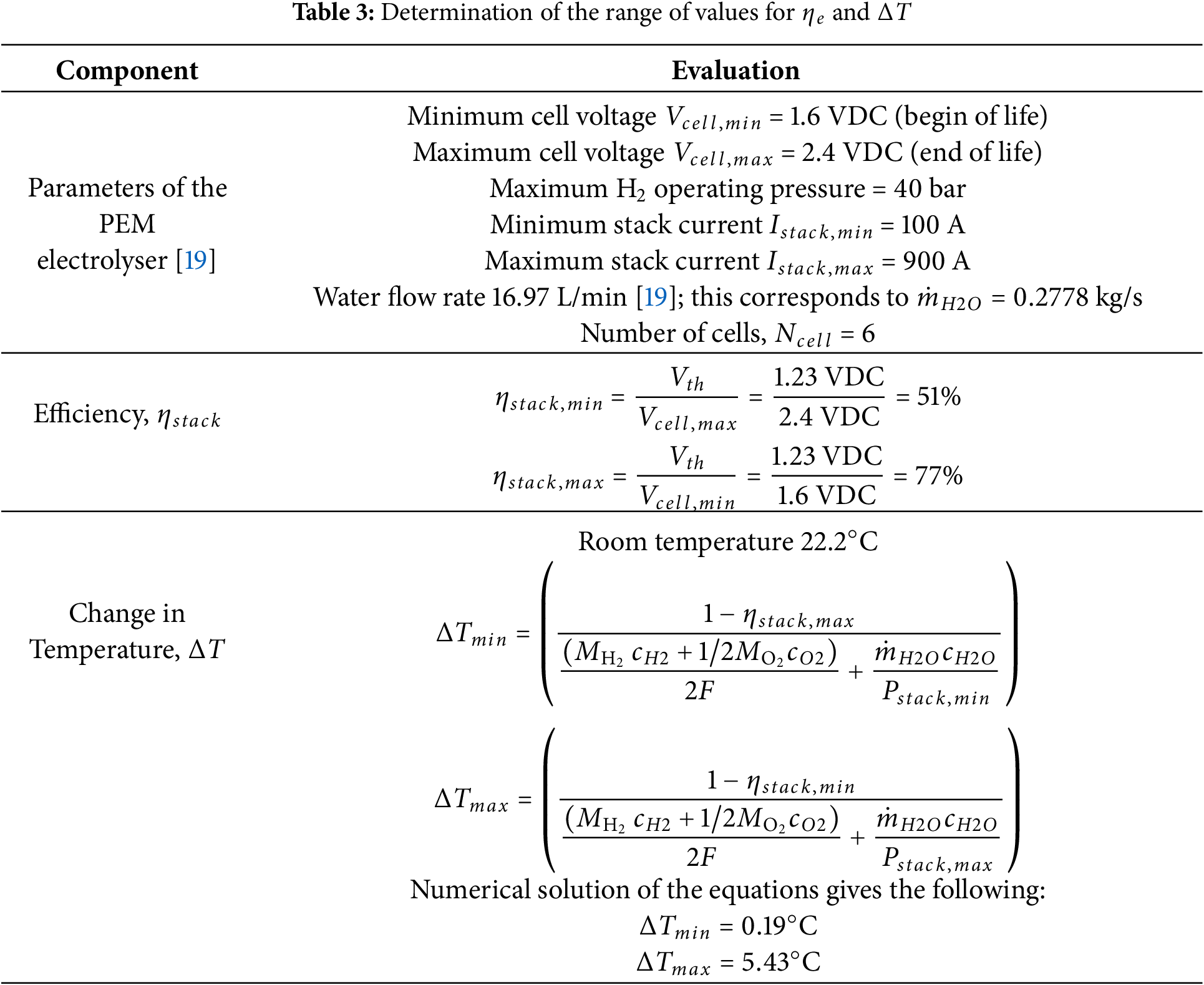
Expression (8) indicates that, when the temperature changes from an initial state, to, to a new state, t, this involves a change in stack efficiency, ηstack. To handle the variables in the fuzzy system, they are normalised as shown in Eqs. (11) and (12).

ηstack¯=ηstackt−ηstack,minηstack,max−ηstack,min(11)

where:

ηstack¯ is the normalised stack efficiency,

ηstackt is the stack efficiency at state t,

ηstack,min is the minimum stack efficiency,

ηstack,max is the maximum stack efficiency.

and (12):

ΔT¯=ΔTt−ΔTminΔTmax−ΔTmin(12)

where:

ΔT¯ is the normalised temperature change,

ΔTt is the change in electrolyser temperature in t (°C),

ΔTmin is the minimum change in electrolyser temperature (°C),

ΔTmax is the maximum change in electrolyser temperature (°C).

From Table 3, it is important to note that the minimum temperature change is 0.19°C and not 0°C as it should ideally be, because the electrolyser is a real machine and part of the energy supplied is dissipated as heat. Also, considering the data from Table 3, Fig. 6a shows a plot of the efficiency dependency on temperature; and a similar plot with normalised values is displayed in Fig. 6b. This second plot is then used along with (8) to define the various fuzzy sets shown in Table 3 and Fig. 7.

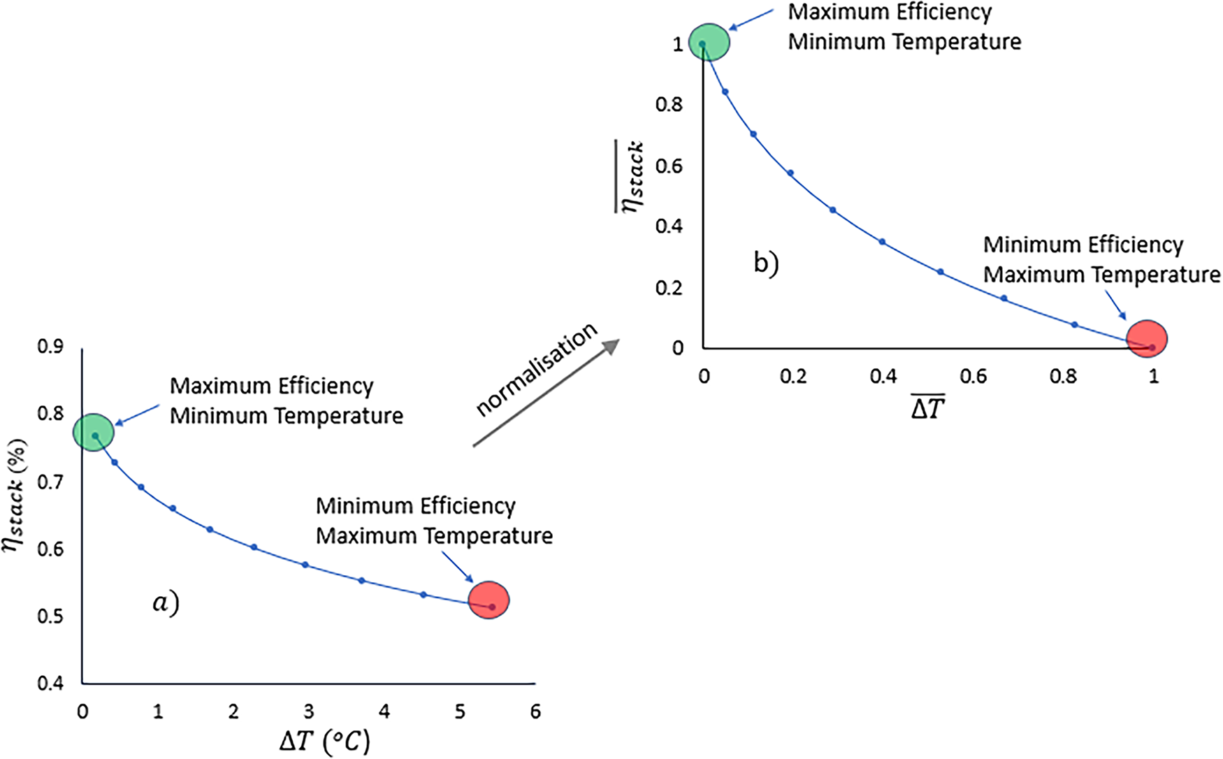
Figure 6: (a) Plot of efficiency (ηstack) with changes in temperature (ΔT). (b) Plot of normalised values of efficiency (ηstack¯) and temperature change (ΔT)¯

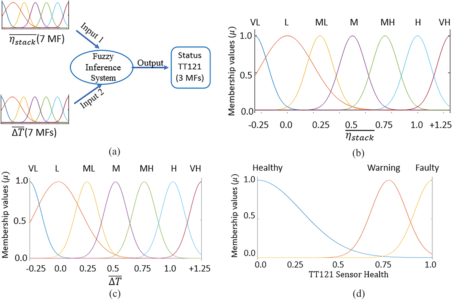
Figure 7: (a) Conceptual scheme of the fuzzy system; (b) ηstack¯ input membership plot; (c) ΔT¯ input membership plot; (d) Hydrogen sensor (TT121) health condition output with membership plot

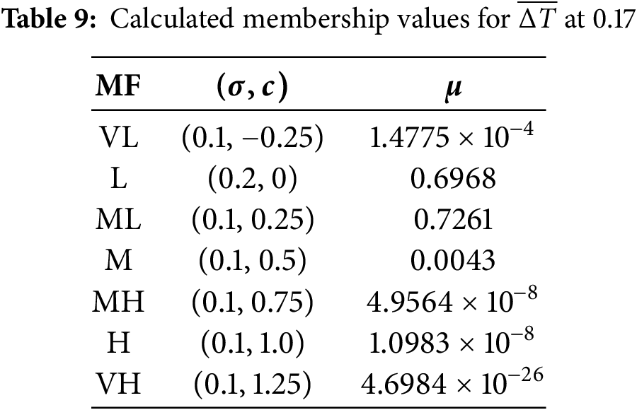
From the plot in Fig. 6b, the range of input values is expected to be within 0 to 1. To design the fuzzy system, we proceed as follows: The input variables to the fuzzy system are required to be well represented by sets which closely match human interpretation. According to Hooda and Raich 2017 [25] human interpretation of measurements can be “very low”, “low”, “slightly low”, “average”, “slightly high”, “high” and “very high”, among others. These are linguistic terms that are very useful for describing to a fuzzy system the possible range of values of each input. The low measurement from one of the inputs will be assigned as the L linguistic variable while the maximum measurement is assigned the H variable. Furthermore, the two extremes of measurement L and H can have a midpoint or average value designated as the M variable in our design. We also use terms to designate measurement that are slightly high but not high. We refer to this variable as medium-high (MH) and another that is slightly low is designated as medium-low (MH). Finally, sensors can fail when they give values much below the lowest and highest values. In these cases, human interpretation can classify this as very low or below range and very high or above range. We classify these additional linguistic variables as VL and VH, respectively. In total, authors have defined 7 linguistic variables for each input variable and they are listed in Table 4. Combinations of each linguistic variable between the two inputs will make a total of 7 × 7 = 49 possibilities which are defined in the matrix called fuzzy rules. Furthermore, the minimum operator will be used for the AND operation in each rule because it is the most computationally efficient. For the output, human interpretation of a sensor condition can be defined as healthy, warning and faulty. The authors’ approach for the output classification is similar to that of Mazzoleni et al. [24].

The seven fuzzy sets are then sorted into intervals of 0.25 (Table 4), with consideration for out-of-range values defined as VL and VH. Indeed, sensor signals can sometimes be out of measuring range, such as the type used in this case study (RS PRO® PT100) with measuring range of −50°C to 250°C, but the operating temperature range is calibrated for the electrolyser from 0°C to 75°C. Sensor measurements below or above the operating range are considered as VL and VH. The ability of the fuzzy system to recognise drift faults that are out of range makes the model very useful for various of sensors.

To facilitate the interpretability of the fuzzy rules, Gaussian membership functions (MFs) will be used for the fuzzification of the variables [26]. The expression for computing the Gaussian membership function of the variables is shown in (13):

μ(x;σ,c)=exp(−(x−c)22σ2)(13)

where:

μ is the membership function of a fuzzy variable at point x

c is the mean where the membership peaks

σ is the standard deviation or degree of overlapping of each membership variable

The overall set of variables are then shown in Table 4.

The inputs and output indicated in Table 4 are subsequently developed in a graphical layout as shown in Fig. 7.

One of the benefits of the developed fuzzy system is that it is more robust and suitable than a threshold-based alarm system because it can handle uncertainties in constants and noise from sensor readings. Overlapping membership functions can easily map small perturbations in the input variables to small changes in the fault belief. This helps to avoid the on/off “chatter” observed with a single threshold.

On the other hand, the electrochemical and thermal coupling of the input variables have a monotonic relationship based on expression (8) such that at a fixed load, a higher true value of temperature lowers the cell voltage through increased ohmic loses and therefore reduced efficiency. A lower true temperature has the opposite effect to this. Because efficiency is derived from voltage signals, it provides a process-based redundancy that is independent of the temperature sensor. The developed fuzzy system implements this parity check through the 49 rules in Table 5. For example, medium to low (ML) temperature data from the temperature sensor along with medium to high (MH) efficiency (rule 19) maps to a healthy sensor condition. Also, incoherent pairs of the signals such as high temperature (H) with high efficiency (H), rule 41, or static state of one of the other variables while the other changes indicate a warning or faulty condition.

The output of the fuzzy system is obtained in steps which are based on the fuzzy-inference system called Mamdani style [26]. The steps are the following:

•   Step 1: Fuzzification of input variables. This converts crisp inputs understandable by human into degrees of membership in linguistic sets that can be used for computation in the rules defined

•   Step 2: Firing of the defined rules. In this step the following takes place:

      º   Each rule has the AND operator for various combination for variables. The function min{µ(ηstack¯)µ(ΔT¯)} is used for each variable combination

      º   Considering strength of rules leading to each output category (Healthy, Warning and Faulty), the max() function is then used to select the greatest contributor for each rule output.

•   Step 3: Implication (clipping of the rule activation)

•   This step maps the truth of the rule’s condition (IF-part) into the strength of its action (THEN-part) so the fuzzy inference process reflects partial truths properly. It basically handles how hard each fired rule pushes on its output shape.

•   Step 4: Aggregation. In this step the combination of each output category that have been clipped in step 3 are combined using the max() function.

•   Step 5: Defuzzification. This is the final step in the Mamdani process, and it uses the bisector method such that the area of the integral of the aggregated outputs to the left equals the area to the right. Then the output value y is at the center defined by the expression (14):

∫01μagg(y)(14)

3.3 Development of the Neural Network

For the development of the neural network, the authors chose an LSTM architecture [15], which is subsequently hybridised with the fuzzy system to produce the AI observer. The main function of the LSTM is to provide a predicted (forecasted) signal of the hydrogen temperature sensor TT121 when it fails.

Based on scientific literature [15], LSTMs are a type of recurrent neural network (RNN) which itself is a subcategory of deep neural networks (DNNs). Then, DNN is a type of supervised learning under machine learning and artificial intelligence concepts. To alleviate the trouble of fading gradients in traditional RNN design, LSTM network is configured from three gates, Fig. 8 where it can store both present and historical information after it has been trained with input data.

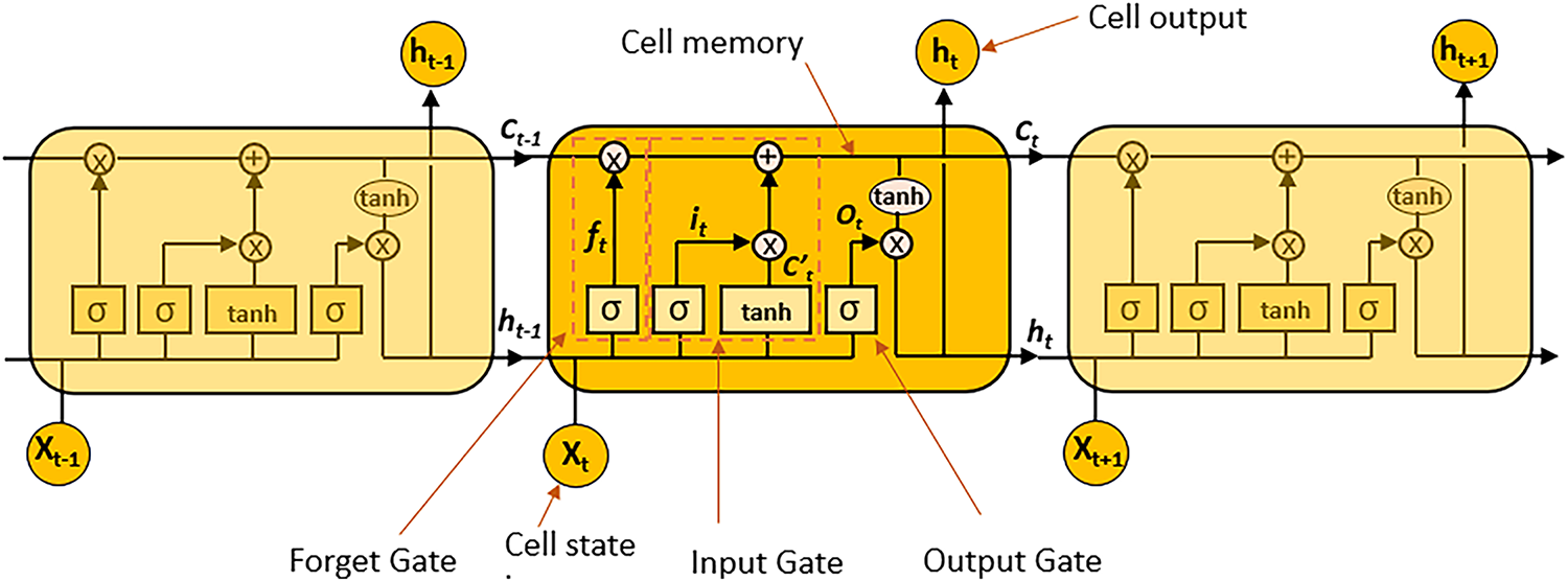
Figure 8: Structure of an LSTM neural network

The relevant equation for each gate of the LSTM are the following:

ForgetGate:ft=σ(Wf.[ht−1,xt]+bf)(15)

InputGate:it=σ(Wi.[ht−1,xt]+bi)(16)

OutputGate:Ot=σ(Wo.[ht−1,xt]+bo)(17)

CandidatevalveCt′=tanh⁡(Wc.[ht−1,xt]+bc)(18)

CellState:Ct=ft∗Ct−1+it∗Ct′(19)

HiddenState:ht=σt∗tanh⁡(Ct)(20)

where:

t is the time step

b is a bias added for each gate

Wf, Wi and Wo are the weight of each gate

ht and ht−1 are the output for the hidden layers in time steps t and t – 1, respectively

xt is the input at time t

σ is the sigmoid activation function

To be able to predict future values, the LSTM needs to be trained. Training time depends on the amount of data available and can range from a few seconds to minutes. The concept of prediction in our solution is the closed loop approach, where predicted values are re-used as old values by the LSTM to predict new(future) values. The first training result is evaluated by checking the root mean square error (RMSE). If it is within an acceptable value (<0.1) [20], then the LSTM is ready for use in the fuzzy-LSTM hybrid model (AI observer) to predict temperature values when a drift fault occurs with the main sensor. If the RMSE is high, the training parameters are adjusted again to obtain an optimum value of RMSE. The entire process is shown in Fig. 9.

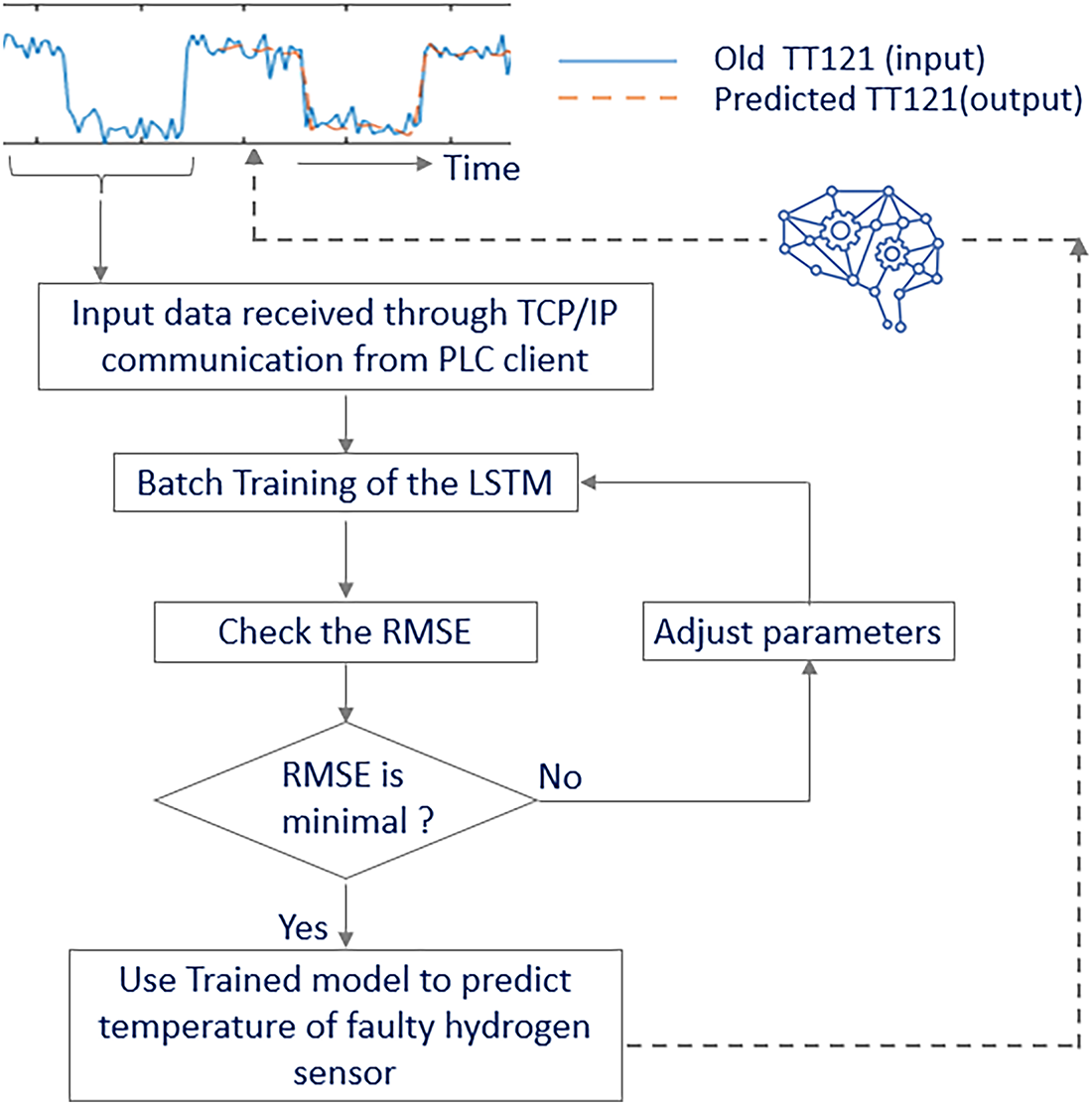
Figure 9: The LSTM neural network for predicting a faulty sensor

The input data for the LSTM are the historical temperature measurements when there was no fault. This data is not readily usable by the LSTM because several time steps share identical values due to stepwise changes. An instance of this problem is shown in Fig. 10 wherein time steps between 1100 and 1200 s have the same value of 23°C. Such a stream of input data gives errors during training of the LSTM and consequently errors in prediction because the neural network is not able to determine differences in temperature over the time steps. However, a workaround approach is to pre-process the data by writing a MATLAB® code to connect the changes at each step together to form a smooth line. Then each timestep will have a unique input data point. The uniqueness of data points is a very important requirement for the accuracy of the LSTM network. Moreover, this approach reduces training time. After smoothing the data, it is normalised to obtain the range 0 to 1.

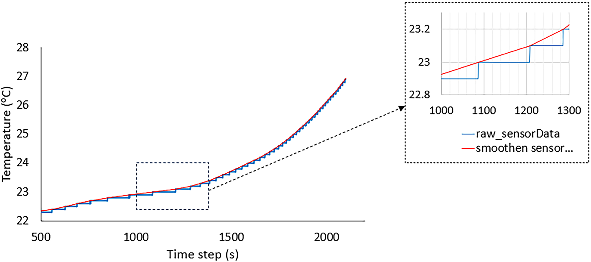
Figure 10: The LSTM neural network for predicting a faulty sensor

For the designed LSTM neural network, historical data are first trained and used to predict a percentage of data points after the occurrence of a fault. The recommended ratio of the training dataset is 75% to 90% while for test data it is 25% to 10% [27]. For this study, drift faults are injected at various points. At a particular time instance, 400 data points are available before the occurrence of a fault. The fault occurs for about 200 data points. These 400 data points are then trained using the training set 1 in Table 6. The trained network is thereafter used to predict 100 data points for the sensor while the drift fault continues to occur. This represents a training-to-prediction ratio of [80:20]. We do not want to predict more than 20% of the data points to avoid increasing the prediction error. As the drift fault continues, the historical data is then added to the predicted data thus making 500 data points. This is then re-trained with the training set 2 in Table 6. The trained network is again used to predict the last batch of 100 data points. The overview of this process is indicated in Fig. 11.

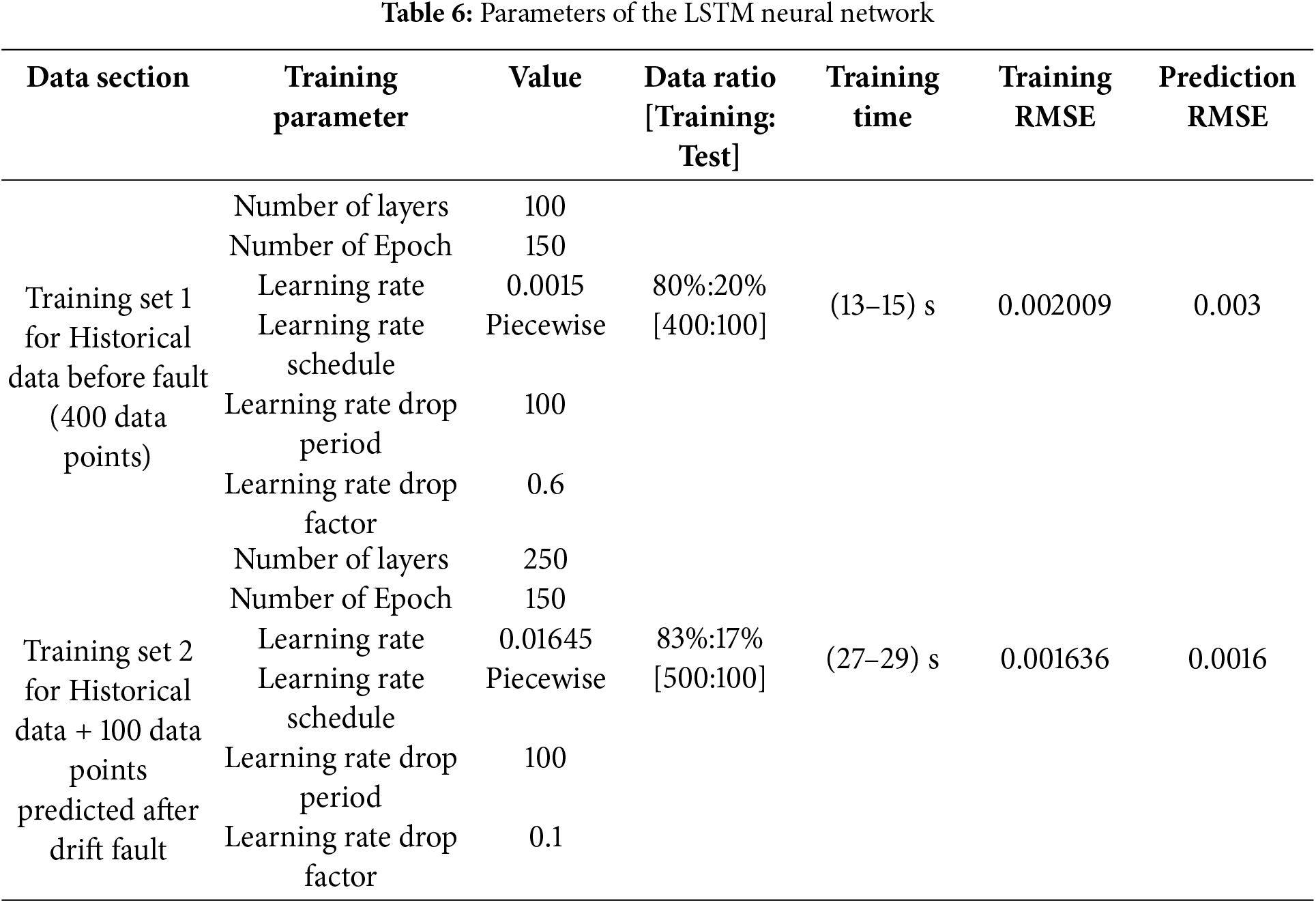
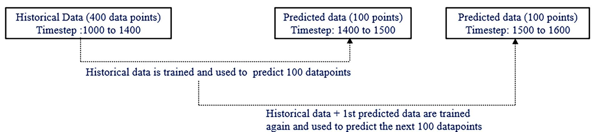
Figure 11: The LSTM neural network for predicting faulty sensor

3.4 Data Exchange in the Developed System

Sensor measurements from the electrolyser [19] are transmitted to the PLC. Then the PLC software (Siemens TIA portal®) is used to set up the hardware configuration to establish TCP/IP communication with a PC running the fuzzy system in MATLAB® as shown in Figs. 12 and 13. The PLC acts as the client while the MATLAB environment acts as the server [28].

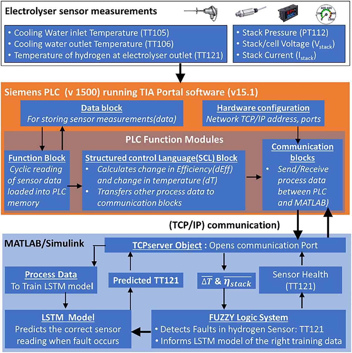
Figure 12: Layout of the data exchange for the proposed solution

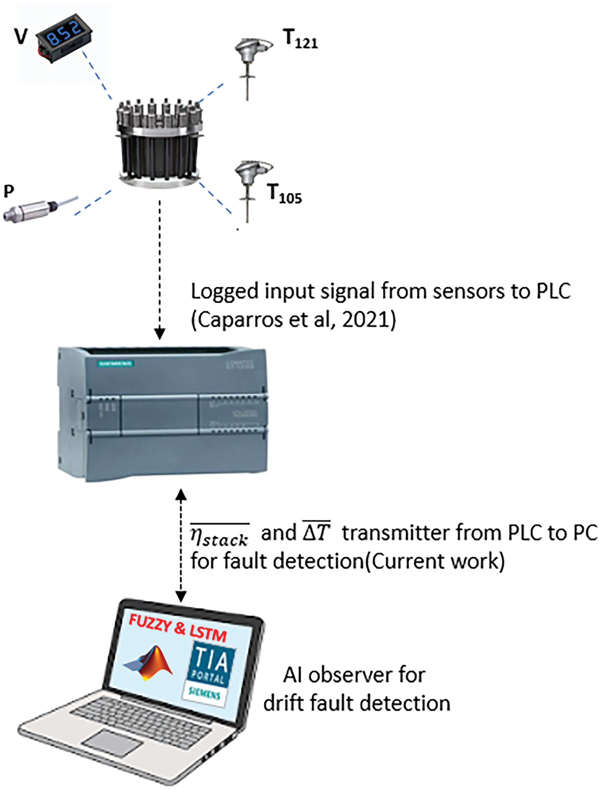
Figure 13: Physical implementation of the PLC and AI observer system [19]

The MATLAB server receives processed sensor data from the PLC client. The processed data are used to formulate fuzzy variables needed to detect drift faults in the hydrogen temperature sensor measurements. The developed fuzzy system considers electrolyser efficiency and hydrogen temperature changes obtained from the client PLC to determine the state of health of the hydrogen temperature sensor, TT121. Additionally, it triggers an alarm that is sent to the PLC client if a drift fault is detected.

In the development of the proposed solution, a continuous data exchange between the PLC and the fuzzy system is implemented in MATLAB®. The developed MATLAB model for the fuzzy system is shown in Fig. 14.

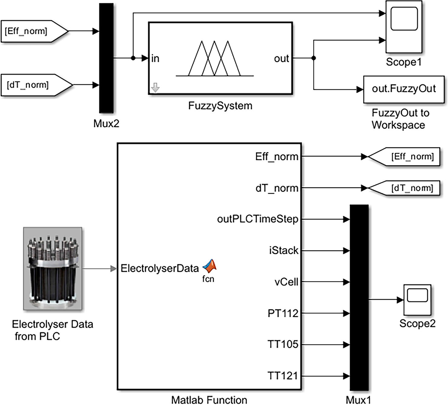
Figure 14: PLC-Fuzzy system integration in MATLAB® Simulink® environment

The electrolyser is put into operation at operating point t, and the cell voltage sensor values, Vcell, are acquired by the PLC to calculate the efficiency, ηstackt using Eq. (9) for each time step. In addition, changes in hydrogen temperature measurements from an initial state, to, to a new state t, are obtained corresponding to the same instance of the efficiency calculated. In the PLC code, the stack efficiency values, and temperature measurements are used in (11) and (12) to compute normalised efficiencies, ηstack¯, and normalised temperature changes, ΔT¯.

These data are then transferred to the fuzzy system in the MATLAB® environment. In return, the fuzzy system generates its evaluation of the hydrogen sensor TT121 health, using fuzzy rules that were previously configured in Section 3.2. When the fuzzy system detects that the sensor state is not healthy, such as a drifting signal, it sends an alarm signal to the PLC, which is subsequently displayed on the operator screen for maintenance action. The software program for the fuzzy system and LSTM run within the MATLAB environment as two separate programs but share data using simple text files.

3.5 PLC Communication with PC

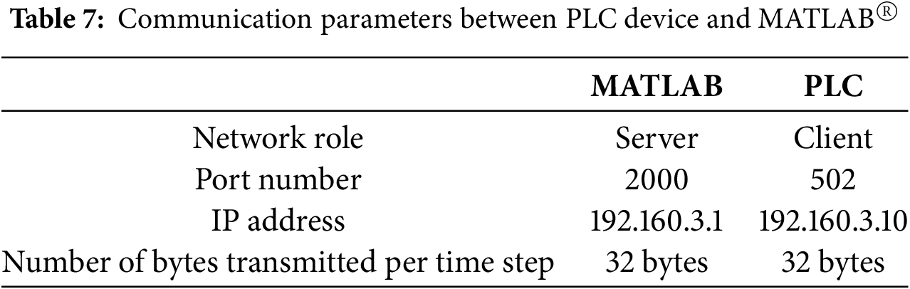
The main parameters to establish communication between the PLC client and the MATLAB® server are shown in Table 7. Communication blocks in the PLC software are created from standard libraries, namely TCON, TSEND, TRCV, and TDISCON, as described in [29]. The IP addresses of the PLC and the PC are linked in each communication block. The port number, the number of bytes to transmit the sensor data, and the client role assigned to the PLC are also defined. On the MATLAB® side, a TCP server object is created as described in [28] with port number 2000. The connection is established when the port is opened on the server. The main libraries used in MATLAB® to communicate, receive, and send data are as follows:

t = tcpserver (‘client address’,2000);        % server object t created

fopen(t);                            % connection opened from MATLAB server

dataIn = fread(t,32);                     %32 bytes sent from client are read by server object

fwrite (t, dataOut);                   % data from fuzzy is sent out to PLC client.

4  Results and Discussion

In this section the developed AI-based observer is tested both for normal and fault induced operation to observe its ability to detect drift faults in the temperature sensor of the electrolyser used in this case study.

4.1 Fine-Tuning the Fuzzy System

An initial test of the fuzzy system shows that it quickly produces output that tends too quickly to the warning zone even when the system is just starting up and temperature is increasing but the efficiency is not changing as much. To dampen this aggressive response, the Gaussian parameter (σ) for the L variable of both inputs in Table 4 are set as σ = 0.2. This makes the coverage of the L variable wider compared to other variables with σ = 0.1. In essence, this adjustment helps to extend the effect of the L variable into the region of ML and M fuzzy sets, such that it acts like a filter to avoid an aggressive reaction of the fuzzy output during onset of drift faults. This effect is shown in Fig. 15, where efficiency is kept constant and then an increasing temperature signal is injected into the fuzzy system to simulate drift fault. For both cases (σ = 0.1 and σ = 0.2) the fault level (defined in the fuzzy rules) was eventually reached. However, for the case when σ = 0.1, the response at the beginning of operation was rather aggressive compared to the case when σ = 0.2, which shows a gradual response due to the filtering effect. For example, at the 10th timestep, the fuzzy output was 0.64 (resulting in a warning health condition) with σ = 0.1; but when σ = 0.2, the fuzzy output was filtered to 0.42 at that time instant.

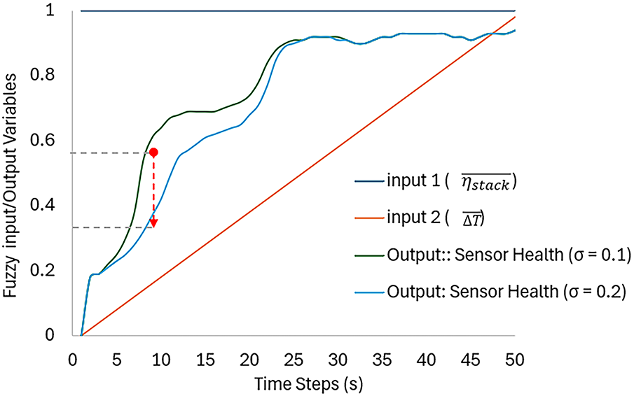
Figure 15: Demonstration of the effect of parameter (σ = 0.2) for the membership function L

4.2 Testing of the PLC-AI Based Observer

The test was started again by using real experimental data logged into the programmable logic controller (PLC) of an electrolyser [19] and transmitted in time steps via Ethernet communication to a remote PC unit running MATLAB® software. During normal operation (no failures), normalised stack efficiency, ηstack¯, and temperature, ΔT¯, were plotted against time steps as shown in Fig. 16a,b. Each time step is represented in seconds, for the logged sensor measurement of which values from 0 to 500 are not plotted since this represents the period of initialisation and purging of the electrolyser. The stack current was increased gradually from 100–900 A with a corresponding increase in voltage. Initial temperature was at 22°C and peaked at around 28°C. Efficiency value at the beginning of electrolyser operation is 77% (ηstack¯∼1) and gradually decreases as temperature increases (ΔT¯ > 0). Continuous exchange of information takes place between the fuzzy system in MATLAB® and the PLC, regarding the sensor health condition and other process data.

Figure 16: (a) Profile of ηstack¯ and (b) Profile of ΔT¯ during normal operation. (c) Response of the fuzzy system referred to hydrogen sensor health in normal operation

The fuzzy outputs in Fig. 16c were activated based on the rules defined in the fuzzy system.

For example, at the time step of 1200, when the input variables are ηstack¯ = 0.91 and ΔT¯ = 0.17, the rules defined in the fuzzy system produced a fuzzy output of 0.39. This value is obtained by following the steps defined in Section 3.2 and herewith calculation for this instance:

Step 1: Using Eq. (13), the fuzzification of the input variables were obtained as follows:

The membership values (μ) of the input variable ηstack¯ at 0.91 are calculated as in Table 8.

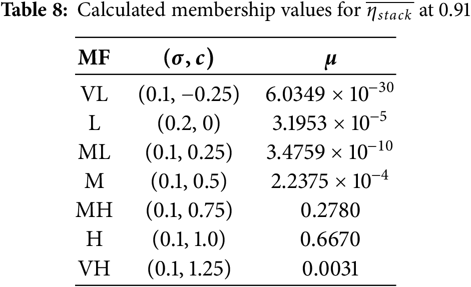
Also, the membership values (μ) of the input variable ΔT¯ at 0.17 are calculated in Table 9.

Step 2: Then, for each rule defined, the min() function is used to compute the AND combination of input variables. Thereafter, the highest combinations were the following:

•   (H and L) ⟶ Healthy: min{0.6670, 0.6968} = 0.6670

•   (H and ML) ⟶ Warning: min{0.6670, 0.7261} = 0.6670

•   (MH and L) ⟶ Warning: min{0.2780, 0.6968} = 0.2780

•   (MH and ML) ⟶ Healthy: min{0.2780, 0.7261} = 0.2780

•   (H and M) ⟶ Faulty: min{0.6670, 0.0043} = 0.0043

•   (VH and L) ⟶ Faulty: min{0.0031, 0.6968} = 0.0031

•   (VH and ML) ⟶ Faulty: min{0.0031, 0.7261} = 0.0031

•   (VH and M) ⟶ Faulty: min{0.0031, 0.0043} = 0.0031

•   (M and L) ⟶ Faulty: min{2.2375 × 10−4, 0.6968} = 2.2375 × 10−4

Then, for the activation of the sensor output, the greatest contributor for each category (Healthy, Warning, Faulty), was obtained as: Healthy = 0.6670, Warning = 0.6670, and Faulty = 0.0043.

The following observations about the rules for the sensor condition are then clear:

º   The “Healthy” and “Warning” condition dominate with a strength of 0.6670.

º   The “No Fault” contribution is negligible at a value of 0.0043.

Step 3: Using Eq. (13) again, the output MF in the range yε[0.1] are obtained as:

º   Healthy: μ1(y)=exp(−(y−0)22∗0.252)

º   Warning: μ2(y)=exp(−(y−0.75)22∗0.12)

Step 4: The main outputs were then aggregated using:

μagg(y)=max{min(exp(−(y−0)22∗0.252),0.6670),min(exp(−(y−0.75)22∗0.12),0.6670)}

º   The healthy condition (centered at 0) is clipped at 0.6670, and

º   Warning (centered at 0.75) is also clipped at 0.6670.

Thus, the effective envelope of the sensor output status was:

º   Healthy (centered at 0 and clipped at 0.667) and

º   Warning (centered 0.75 and clipped at 0.667).

Step 5: The defuzzification step uses the bisector defined in Eq. (14). Then,

12∫01μagg(y)=0.39

This fuzzy output of 0.39 represents the sensor condition at the instance of the input variables (ηstack¯ = 0.91 and ΔT¯= 0.17).

All other fuzzy outputs are then computed in MATLAB using these steps for each pair of input combination.

Based on the developed fuzzy system, it is noted from Fig. 16b that during the beginning of operation up to the time step, 1200 s, the signals generated by the fuzzy system tended towards the warning zone. This is because, from Fig. 16a the normalised change in temperature ΔT¯ was increasing at a faster rate compared to the drop in normalised efficiency ηstack¯ which is often experienced when the system is starting to operate. Then at time step t > 1200 s, ηstack¯ starts to decrease at a rate comparable with ΔT¯, meaning that the electrolyser temperature is ramping up. This performance matches with normal operation. The fuzzy system output advises that the sensor reading is healthy. In some times, t = [1400, 1700, 2000, 2150 min], it can be observed that the fuzzy system output notifies of a potential problem with the sensor health condition, Fig. 16c. This is explained because at these points, the efficiency remains almost constant. If the efficiency doesn’t change, neither should the temperature; otherwise, this is an indicator of the sensor health is being harmed.

In the second test, Fig. 17, drift fault signals, δ, with a half-wave sine profile between t = [600 to 800 s] and t = [1400 to 1600 s] were introduced into the hydrogen temperature measurement TT121 as shown in Fig. 17b. Failure signals cause (ΔT¯+δ1) to rise to 0.7 in the first case, and (ΔT¯−δ2) drop to −0.5 in the second one. These deviations (drift-type faults) during the normal operation of the electrolyser, are detected by the AI-based observer, which produces warnings and alarms for each case, as indicated in Fig. 17c.

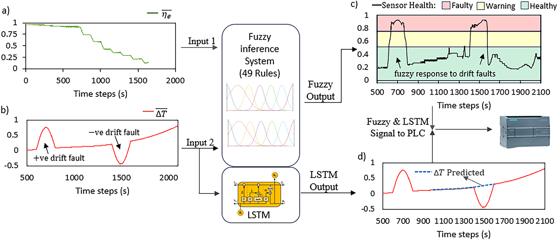
Figure 17: (a) Profile plot of ηstack¯and (b) ΔT¯ during drift-type fault at two different instances. (c) Response of the fuzzy system to the drift-type sensor faults. (d) Predicted output from the LSTM

Once the faults disappear, as demonstrated at t = 800 and 1600 s, the fuzzy system indicates that the sensor reading has returned to healthy operation. It is important to note that during the occurrence of the second fault as shown in Fig. 17d, the LSTM neural network begins to provide predicted data (hydrogen temperature TT121) which are normalised within the range of 0 to 1 in the same manner as the input signal. Predicted data are useful to the control system to allow the electrolyser to continue operating while the faulty sensor is planned for replacement or maintenance action. The predicted values from the LSTM were initially not available at the early stage of electrolyser operation until around t ≥ 1000 s. This is because the LSTM requires significant training data and time before predicting future values of temperature.

The prediction occurs in two phases as previously explained in Section 3.3 and Fig. 11. Before timestep t = 1000 s, the system had not acquired sufficient and fault-free data for training. The occurrence of a fault between timestep 600 to 800 s requires the program code to wait until normal data resumes. At timestep 1000 to 1400 s there is sufficient fault free data to train the LSTM online. The training was done within 13 to 15 s, which is fast enough to allow rapid commencement of prediction after training. The first batch of training produces 100 data points which represent 20% of the training data. Predicted values per time step are re-used as old input data by the LSTM to predict new values in a closed loop. The plot of the first prediction from timestep t = 1400 to 1500 s is shown in Fig. 18a. It was previously mentioned in Section 3.3 that the LSTM should not predict more than 20% of training data to avoid compounding errors which affects accuracy. Hence, our approach is to incorporate within the MATLAB program code, the merging of the predicted data points (100) with the old data points (400) and then re-train the combined data. The second training was done within 27 s after which the LSTM was ready for use to predict the next data points. At timestep 1500 s, another batch of prediction began until step t = 1600 s, which also corresponded to the time the injected drift fault is cleared. Predicted data points for the batches are shown in Fig. 18b as plotted from MATLAB®. The overall stages of predictions were carried out online and automatically using program code developed for the AI-observer.

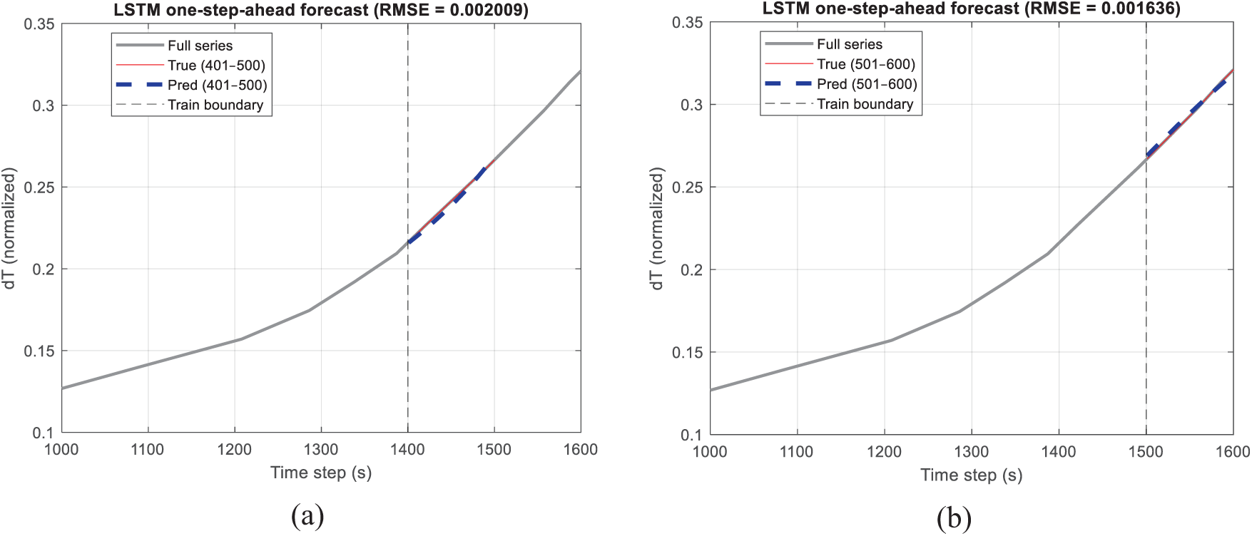
Figure 18: (a) Plot of predicted temperature signal by LSTM at t = 1400 to 1500 s. (b) Plot of predicted temperature signal by LSTM at t = 1500 to 1600 s

Another test was done with a slow-moving drift fault as shown in Fig. 19. In Fig. 19a, a positive drift fault was injected slowly which is a common occurrence with sensors in real world applications. Also, in Fig. 19b, another test was done with a negative and slow drift fault. The results of the two tests are shown in Fig. 19c,d, where the fuzzy system was able to detect each drift fault at about timestep of 1200 s. This shows again the capability of the developed AI-observer to detect even very slow drift type of fault.

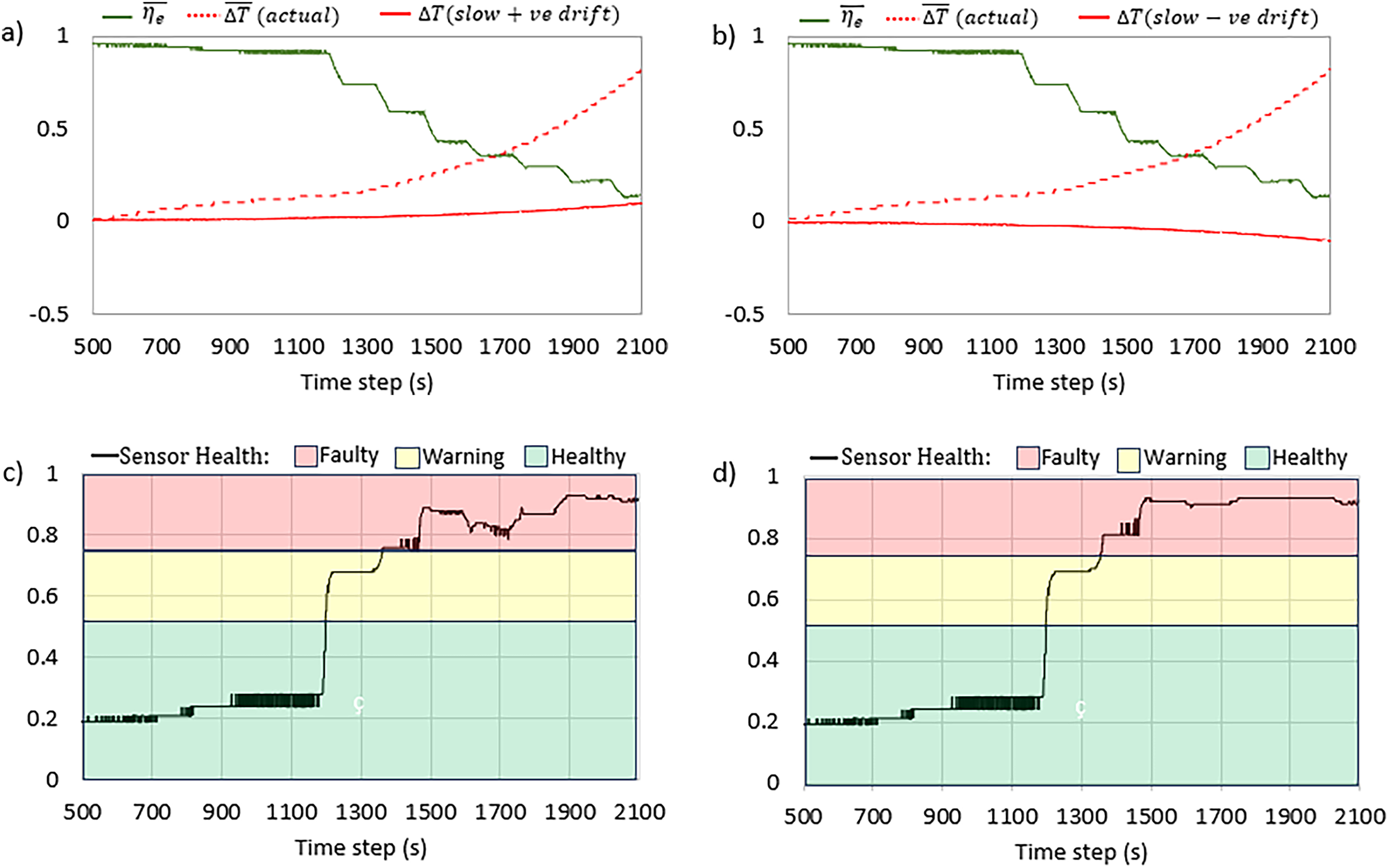
Figure 19: (a) Introduction of slow and positive drift fault. (b) Introduction of negative and slow drift fault. (c) Response of the AI-observer to the positive drift fault. (d) Response of the AI-observer to the negative drift fault

4.3 Fuzzy Rules Validation

Finally, the fuzzy rules defined for the AI-based observer are validated using the experimental electrolyser data. Fig. 20 shows the numerical data obtained from the developed fuzzy system and the experimental data. The plots illustrate the relationship between efficiency and temperature changes. A comparison with the numerical data in Fig. 6 shows that the rules of the fuzzy component of the AI-based observer guarantee an accuracy of ±0.25 within the range 0 to 1, as indicated by the region marked “OK”. Any sensor signal measurement outside the normal zone will trigger a warning or fault in the fuzzy system. Furthermore, Fig. 20 reveals a clear model–plant mismatch since the numerical trend between efficiency and temperature changes fitted to the experimental data (dashed line; see legend) departs systematically from the theoretical curve used to design the fuzzy rules. This deviation persists across the operating range, indicating that thresholds derived from the nominal model alone would misclassify a non-negligible set of operating points near the decision boundaries. In practice, measurement noise, unmodelled losses, and aging effects shift the plant away from the idealized relationship. This is precisely where the proposed fuzzy logic scheme adds value. By replacing crisp thresholds with overlapping membership functions, the classifier tolerates imprecision and handles uncertainty around the boundaries while classifying the operating region of the sensor as Healthy (OK), Warning and Faulty, based on the fuzzy rule combination.

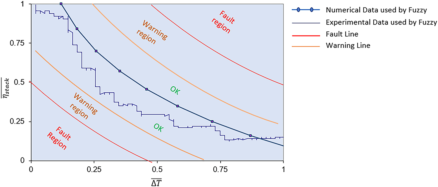
Figure 20: Comparison of the profile used to tune the output of the fuzzy system with experimental data

5  Conclusions

This paper demonstrates the development of an AI-based observer for use in predictive maintenance. It integrates the operation of a PLC with a fuzzy system and an LSTM neural network to detect abnormalities in the temperature sensor of an electrolyser plant. It is important to note that, unlike previous works, the developed system does not rely on training or historical fault data before detecting drift faults in the sensor. The drift fault detection enables maintenance personnel to plan for the replacement or recalibration of the affected sensor accordingly. If sufficient process data has been acquired prior to the sensor fault, the LSTM can then take over by providing predicted sensor data to the control system so that the system continues to operate while the faulty sensor is planned for corrective action. The AI-based observer is also better than conventional alarm systems, which mainly detect faults only after the sensor has failed. The potential hazard is that an unidentified erroneous measurement can prevent the electrolyser cooling system from responding in a timely manner, which can lead to irreversible damage to the electrolyser.

Overall, the developed combined AI-based observer enhances the durability of the electrolyser, as faults such as measurement drift are quickly detected and corrected before failure occurs. Of course, the methodology and system developed can be used in other types of hydrogen-based plants, where maintenance is critical to reduce operation and management costs as well as replacement costs, thereby extending the useful life of equipment. The main limitation of the authors’ proposal is that, for a given system, there is no reliable theoretical model available that allows modelling and fault detection using fuzzy rules. That is, the fuzzy model is not reliable. Another limitation is the system’s sensorization: inadequate sensors (which should be resolved beforehand), an unreliable or insufficiently representative dataset, or weak correlations that hinder the training of the neural network. Future work will provide solutions to these challenges and align with an emerging trend in the use of explainable AI [16,17] by keeping fuzzy logic as a white box system for safety and traceability while configuring a deep expert network (DEN) to learn or refine rule weights and thresholds from data.

Acknowledgement: Not applicable.

Funding Statement: This work has been partially carried out thanks to the support of (1) Grant Ref. PID2023-148456OB-C41 and (2) Grant Ref. RED2022-134588-T found by MICIU/AEI/10.13039/501100011033.

Author Contributions: The authors confirm contribution to the paper as follows: Conceptualization, Abiodun Abiola and Francisca Segura; methodology, Abiodun Abiola; software, Abiodun Abiola; validation, Abiodun Abiola and Francisca Segura; formal analysis, Abiodun Abiola, Francisca Segura, Antonio Barragán and José Manuel Andújar; investigation, Abiodun Abiola, Francisca Segura, Antonio Barragán and José Manuel Andújar; resources, Abiodun Abiola and Francisca Segura; data curation, Abiodun Abiola, Francisca Segura and Antonio Barragán; writing—original draft preparation, Abiodun Abiola and Francisca Segura; writing—review and editing, Abiodun Abiola, Francisca Segura, Antonio Barragán and José Manuel Andújar; visualization, Abiodun Abiola and Francisca Segura; supervision, José Manuel Andújar; project administration, Francisca Segura and Antonio Barragán; funding acquisition, José Manuel Andújar. All authors reviewed the results and approved the final version of the manuscript.

Availability of Data and Materials: The data that support the findings of this study are available from the corresponding author upon reasonable request.

Ethics Approval: Not applicable.

Conflicts of Interest: The authors declare no conflicts of interest to report regarding the present study.

References

1. Agredano-Torres M, Zhang M, Söder L, Xu Q. Decentralized dynamic power sharing control for frequency regulation using hybrid hydrogen electrolyzer systems. IEEE Trans Sustain Energy. 2024;15(3):1847–58. doi:10.1109/tste.2024.3381491. [Google Scholar] [CrossRef]

2. Rey J, Segura F, Andújar JM, Ferrario AM. The economic impact and carbon footprint dependence of energy management strategies in hydrogen-based microgrids. Electronics. 2023;12(17):3703. doi:10.3390/electronics12173703. [Google Scholar] [CrossRef]

3. Lebbal ME, Lecoeuche S. Identification and monitoring of a PEM electrolyser based on dynamical modelling. Int J Hydrogen Energy. 2009;34(14):5992–9. doi:10.1016/j.ijhydene.2009.02.003. [Google Scholar] [CrossRef]

4. Zhao D, He Q, Yu J, Guo M, Fu J, Li X, et al. A data-driven digital-twin model and control of high temperature proton exchange membrane electrolyzer cells. Int J Hydrogen Energy. 2022;47(14):8687–99. doi:10.1016/j.ijhydene.2021.12.233. [Google Scholar] [CrossRef]

5. Folgado FJ, González I, Calderón AJ. Data acquisition and monitoring system framed in Industrial Internet of Things for PEM hydrogen generators. Internet Things. 2023;22:100795. doi:10.1016/j.iot.2023.100795. [Google Scholar] [CrossRef]

6. Wang H, Zhang W, Yang D, Xiang Y. Deep-learning-enabled predictive maintenance in industrial Internet of Things: methods, applications, and challenges. IEEE Syst J. 2023;17(2):2602–15. doi:10.1109/jsyst.2022.3193200. [Google Scholar] [CrossRef]

7. Zhang W, Yang D, Wang H. Data-driven methods for predictive maintenance of industrial equipment: a survey. IEEE Syst J. 2019;13(3):2213–27. doi:10.1109/jsyst.2019.2905565. [Google Scholar] [CrossRef]

8. Gorenstein A, Kalech M. Predictive maintenance for critical infrastructure. Expert Syst Appl. 2022;210:118413. doi:10.1016/j.eswa.2022.118413. [Google Scholar] [CrossRef]

9. Zhao X, Fang Y, Min H, Wu X, Wang W, Teixeira R. Potential sources of sensor data anomalies for autonomous vehicles: an overview from road vehicle safety perspective. Expert Syst Appl. 2024;236:121358. doi:10.1016/j.eswa.2023.121358. [Google Scholar] [CrossRef]

10. da Silva JC, Saxena A, Balaban E, Goebel K. A knowledge-based system approach for sensor fault modeling, detection and mitigation. Expert Syst Appl. 2012;39(12):10977–89. doi:10.1016/j.eswa.2012.03.026. [Google Scholar] [CrossRef]

11. Kajmakovic A, Diwold K, Römer K, Pestana J, Kajtazovic N. Degradation detection in a redundant sensor architecture. Sensors. 2022;22(12):4649. doi:10.3390/s22124649. [Google Scholar] [PubMed] [CrossRef]

12. Kaufmann M, Meier A, Stoffel K. IFC-Filter: membership function generation for inductive fuzzy classification. Expert Syst Appl. 2015;42(21):8369–79. doi:10.1016/j.eswa.2015.06.034. [Google Scholar] [CrossRef]

13. Son JD, Niu G, Yang BS, Hwang DH, Kang DS. Development of smart sensors system for machine fault diagnosis. Expert Syst Appl. 2009;36(9):11981–91. doi:10.1016/j.eswa.2009.03.069. [Google Scholar] [CrossRef]

14. Athanasopoulou C, Chatziathanasiou V. Intelligent system for identification and replacement of faulty sensor measurements in Thermal Power Plants (IPPAMAS: part 1). Expert Syst Appl. 2009;36(5):8750–7. doi:10.1016/j.eswa.2008.12.057. [Google Scholar] [CrossRef]

15. Hochreiter S, Schmidhuber J. Long short-term memory. Neural Comput. 1997;9(8):1735–80. doi:10.1162/neco.1997.9.8.1735. [Google Scholar] [PubMed] [CrossRef]

16. Ali S, Abuhmed T, El-Sappagh S, Muhammad K, Alonso-Moral JM, Confalonieri R, et al. Explainable Artificial Intelligence (XAIwhat we know and what is left to attain Trustworthy Artificial Intelligence. Inf Fusion. 2023;99:101805. doi:10.1016/j.inffus.2023.101805. [Google Scholar] [CrossRef]

17. Li Q, Liu Y, Sun S, Qin Z, Chu F. Deep expert network: a unified method toward knowledge-informed fault diagnosis via fully interpretable neuro-symbolic AI. J Manuf Syst. 2024;77:652–61. doi:10.1016/j.jmsy.2024.10.007. [Google Scholar] [CrossRef]

18. Wang CR, Stansberry JM, Mukundan R, Chang HJ, Kulkarni D, Park AM, et al. Proton exchange membrane (PEM) water electrolysis: cell-level considerations for gigawatt-scale deployment. Chem Rev. 2025;125(3):1257–302. doi:10.1021/acs.chemrev.3c00904. [Google Scholar] [PubMed] [CrossRef]

19. Caparrós JJ, Vivas FJ, Segura F, Andújar JM. Optimized balance of plant for a medium-size PEM electrolyzer. Design, modelling and control. SNE Simul Notes Eur. 2021;31(3):133–41. doi:10.11128/sne.31.tn.10574. [Google Scholar] [CrossRef]

20. Abiola A, Manzano FS, Andújar JM. A novel deep reinforcement learning (DRL) algorithm to apply artificial intelligence-based maintenance in electrolysers. Algorithms. 2023;16(12):541. doi:10.3390/a16120541. [Google Scholar] [CrossRef]

21. Chandesris M, Médeau V, Guillet N, Chelghoum S, Thoby D, Fouda-Onana F. Membrane degradation in PEM water electrolyzer. Int J Hydrogen Energy. 2015;40(3):1353–66. doi:10.1016/j.ijhydene.2014.11.111. [Google Scholar] [CrossRef]

22. Zini G, Tartarini P. Solar hydrogen energy systems. Milan, Italy: Springer; 2012. doi:10.1007/978-88-470-1998-0. [Google Scholar] [CrossRef]

23. Bessarabov D, Millet P. Fundamentals of water electrolysis. In: PEM water electrolysis. Amsterdam, The Netherlands: Elsevier; 2018. p. 43–73. doi:10.1016/b978-0-12-811145-1.00003-4. [Google Scholar] [CrossRef]

24. Mazzoleni M, Sarda K, Acernese A, Russo L, Manfredi L, Glielmo L, et al. A fuzzy logic-based approach for fault diagnosis and condition monitoring of industry 4.0 manufacturing processes. Eng Appl Artif Intell. 2022;115:105317. doi:10.1016/j.engappai.2022.105317. [Google Scholar] [CrossRef]

25. Hooda DS, Raich V. Fuzzy logic models and fuzzy control. Oxford, UK: Alpha Science International Ltd.; 2017. [Google Scholar]

26. Vélez MÁ., Sánchez O, Romero S, Andújar JM. A new methodology to improve interpretability in neuro-fuzzy TSK models. Appl Soft Comput. 2010;10(2):578–91. doi:10.1016/j.asoc.2009.08.027. [Google Scholar] [CrossRef]

27. Hudson M, Martin B, Hagan T, Demuth HB. Deep learning ToolboxTM user’s guide. Natick, MA, USA: MathWorks Inc. [cited 2025 Sep 19]. Available from: https://www.mathworks.com/help/pdf_doc/deeplearning/nnet_ug.pdf. [Google Scholar]

28. MathWorks Inc. Instrument control ToolboxTM user’s guide R2024a. Natick, MA, USA: MathWorks Inc. [cited 2025 Sep 19]. Available from: https://www.mathworks.com/help/pdf_doc/instrument/instrument_ug.pdf. [Google Scholar]

29. Siemens AG. STEP 7 and WinCC engineering system manual v15. Nürnberg, Germany: Siemens AG. [cited 2025 Sep 19]. Available from: https://cache.industry.siemens.com/dl/files/202/109755202/att_940497/v1/STEP_7_WinCC_V15_1_enUS_en-US.pdf. [Google Scholar]