An Isothermal Surface Imaging and Transfer Learning Framework for Fast Isothermal Surface Prediction and 3D Temperature Field Reconstruction in Metal Additive Manufacturing

1  Introduction

Metal additive manufacturing (AM) technology has attracted promising applications in many fields due to its ability to fabricate parts with complex geometries and enable rapid customization. As one of the key metal AM technologies, the laser powder bed fusion (LPBF) process utilizes a high-energy laser beam that moves along predefined scan paths to melt metal powder in a track-by-track, layer-by-layer manner. The thermal behavior during the process, characterized by high thermal gradients and rapid cooling rates [1–3], is closely related to the quality and efficiency of the fabrication. In particular, complex thermal evolution can lead to the formation of manufacturing defects, such as surface inhomogeneity and internal porosity. Therefore, rapid prediction of the temperature field is essential for online process control to ensure component quality and fabrication efficiency in LPBF.

Although traditional numerical methods, including the finite element method (FEM) and the finite volume method (FVM), have been widely developed to simulate transient temperature fields [4–6], their practical applications remain constrained by prohibitive computational costs, especially under fine spatiotemporal resolution requirements. In contrast, machine learning methods automatically learn hierarchical representations from data offline and then make real-time predictions online. However, this advantage in efficiency often comes at the cost of relying heavily on large-scale labeled samples, which is expensive to achieve by either experimental measurements or high-fidelity simulations. Therefore, it remains an open problem to develop a machine learning based method using small samples to efficiently predict the 3D temperature field during the metal AM process.

Many efforts have been devoted to machine learning (ML) models for AM. These works can be divided into two categories: the physics-driven ML models and the data-driven ML models. Compared with the latter, the former is directly used to solve the partial differential equations (PDEs) without or with a little dependence on labeled samples. For example, the physics-informed neural network (PINN) model [7–9], using the residual of the governing equation of the physical problem as a loss function, is the most representative. Zhu et al. [7] first extended the PINN model to metal AM processes to predict the temperature and the molten pool flow fields. The model was trained on a small subset of high-fidelity finite element simulation data (spanning 1.2 to 1.5 ms) and achieved relative discrepancies of 2.9% to 9.7% for the dimensions of the molten pool and 7.8% to 37.7% for the cooling rates compared to NIST AM-Benchmark experimental measurements. However, the computational efficiency of the PINN is shown to be lower than that of FEM. Li et al. [10] proposed a label-free PINN model that incorporates heat conduction, convection, and radiation equations to predict 3D temperature fields for the laser metal deposition process. The model achieved a maximum relative error of approximately 2% (with mean relative errors ranging from 0.64% to 0.95%) compared to the FEM results. In terms of computational efficiency, the basic training process took approximately 650 s on Nvidia A100 GPUs, while the FEM simulation required 600 s on a 12-core i7-12700K CPU. Liao et al. [11] developed a hybrid physics-based data-driven PINN to predict the full-field temperature history and identify unknown parameters in AM by combining partially observed data with heat conduction laws. For the bare plate scanning example, the PINN achieved a root mean square error (RMSE) of 14.07 K compared to the FEM results, which was further reduced to 3.72 K when incorporating noisy auxiliary data, and took approximately 2.5 h on an RTX A6000 GPU. To enable real-time prediction, recent studies have shifted towards data-driven PINNs, referred to as the parametric PINNs, which are trained offline and makes predictions online. By integrating process parameters directly into the model input, these models can predict temperature fields for unseen conditions without updating weights. Hosseini et al. [12] used a parametric PINN model for the prediction of transient temperature fields and the dimensions of the molten pool. The model achieved a mean absolute error (MAE) below 4.5% for temperature predictions compared to FEM benchmarks. Although the PINN training process took approximately 1.8 h (constant properties) to 4 h (temperature-dependent properties) on a single Nvidia Titan RTX GPU compared to 0.2 to 2.5 h for the corresponding FEM simulations on a 12-thread Intel Xeon Gold 6150 CPU, the trained PINN model achieved a prediction at the cost of around 1 ms. Xie et al. [13] proposed a parametric PINN model to predict the 3D temperature fields for the direct energy deposition (DED) process, where 6000 samples generated from a high-fidelity finite element model were used, and the model achieved a mean relative error of 4.83% compared to experimental measurements (with mean relative errors between 0.8% and 3.5% compared to the FEM results) within a mean prediction time of 0.20 ms. Although parametric PINN can perform real-time prediction, it suffers from the same shortcomings as data-driven ML models with multilayer neural networks, as discussed below. Moreover, the original PINN, which directly solves PDEs, is not suitable for the real-time analysis of physical problems [14].

Data-driven ML models have been widely used for predicting the temperature field in AM due to their effectiveness in learning complex nonlinear mappings from data [15–17]. Compared with PINN, they avoid the physics-based constraints and associated automatic differentiation during offline training, while achieving efficient prediction once trained. For example, Roy and Wodo [18] proposed an artificial neural network-based surrogate model to predict the temperature history in the fused filament fabrication process, where a total of 26,000 training data points from 3D cuboid geometries with a fixed cross-section of 2.4×2.4 mm2 and lengths ranging from 2.0 to 6.0 mm, discretized with a mesh size of 0.1 mm, were generated using the transient heat conduction FEM. The model achieved a prediction accuracy exceeding 95% with a computational cost of approximately 326 per simulation (0.036 s per point) executed on a single-core Intel Xeon E5645 CPU @ 2.40 GHz, which can take up to 35.5 h using FEM executed on a 12-CPU system. Pham et al. [19] proposed a feedforward neural network-based surrogate model to predict the temperature field in the DED process. The model was trained on 19.92 million samples generated using a 2D heat conduction FEM model. The domain was discretized into 2519 nodes via a non-uniform mesh: a fine 0.7 mm mesh was applied to the cladding, while the substrate bottom featured a coarse mesh. The surrogate model achieved a prediction accuracy of 99% with a computational cost of 12 s per simulation, and the FEM model takes 0.6 h. It is clear that a direct mapping from the process input to the high-dimensional temperature field via a deep learning neural network requires a massive number of training samples. Because high-fidelity numerical simulations are time-consuming, these existing data-driven models often rely on the simulation data from the simplified numerical models with coarse mesh, in which many thermofluid flow effects, e.g., the molten pool convection, are ignored. The promising data-driven ML model should be trained using samples with high fidelity and fine spatial resolution. However, the limited availability of expensive high-fidelity simulation data challenges the data-driven ML model using neural networks for fast prediction of temperature fields in metal AM.

To address the aforementioned challenge, we proposed an isothermal surface imaging and transfer learning (ISI-TL) framework for rapid and accurate prediction of the isothermal surface and the reconstruction of the 3D temperature field in metal AM. The proposed framework is formulated for application within the stable LPBF processing window. Unlike data-driven ML models that directly output voxel temperatures, the proposed ML model in the framework outputs the geometric morphology of isothermal surfaces, which are further aggregated to construct the 3D temperature field. To this end, a physics-guided isothermal surface imaging method is used to transform the high-dimensional 3D problem into a low-dimensional 2D one, decomposing the temperature field of interest into a finite set of isothermal surfaces. These isothermal surfaces are further compressed along the build direction into a 2D grayscale image, achieving an efficient structured representation of the temperature field. Then, a pre-trained hybrid parameter-to-image generative neural network (PHPG-NN) is trained to predict 2D grayscale images with process parameters as input. A strategy of combining unsupervised and supervised learning is used to maximize the extraction and utilization of information from limited data. Once a PHPG-NN is trained for one isothermal surface, a transfer learning is used to extend it to other isothermal surfaces corresponding to different temperature values by a lightweight fine-tuning step, rather than retraining the entire complex NN. A combination of PHPG-NNs trained on different isothermal surfaces can yield a 3D temperature field for a region of interest via spatial interpolation among a set of isothermal surfaces, thereby enabling scalable temperature prediction. The proposed PHPG-NN and the entire framework are trained and validated using 100 samples, generated with a high-fidelity numerical model using the multiphysics material point method (MPM), which is validated against experimental data. The predicted results for unseen samples agree well with those from high-fidelity numerical simulations, while the computational efficiency of the PHPG-NN is shown to be orders of magnitude higher than that of the multiphysics MPM.

The remainder of this paper is organized as follows. In Section 2, we present the proposed ISI-TL framework, including the high-fidelity numerical model to generate training samples, the physics-guided isothermal surface imaging method, and the PHPG-NN with its transfer learning strategy for the isothermal surface prediction and the reconstruction of the 3D temperature field. Section 3 presents the prediction results of the proposed framework, demonstrating its accuracy and efficiency with limited samples. Finally, Section 4 makes concluding remarks and lists future research directions.

2  Isothermal Surface Imaging and Transfer Learning Framework

In this section, the proposed ISI-TL framework is introduced for rapid prediction of a high-dimensional nonlinear temperature field with scarce high-fidelity simulation data. As illustrated in Fig. 1, the framework adopts a high-fidelity thermo-fluid flow model to obtain 3D temperature fields under various process parameters, then utilizes the physics-guided isothermal surface imaging method to convert the 3D temperature field within the region of interest (ROI) for a given time instance into a series of 2D grayscale images, which are further normalized and divided into training and testing samples for the PHPG-NN model. The PHPG-NN model, consisting of a deep neural network (DNN) and a convolutional neural network (CNN) decoder, establishes a direct mapping from the process parameters to the geometric morphology of the isothermal surface of T. Given the significant influence of laser power (P) and scanning speed (V) on molten pool dynamics, these two parameters are selected as the model inputs. Once trained, a set of PHPG-NNs is constructed through transfer learning for different isothermal surfaces within the same ROI. For a new set of process parameters, multiple PHPG-NNs are used simultaneously to predict the corresponding isothermal surfaces, from which a 3D temperature field within the ROI can be reconstructed via spatial interpolation. The high-fidelity thermo-fluid flow model and each part of the ISI-TL framework are detailed in the following sections.

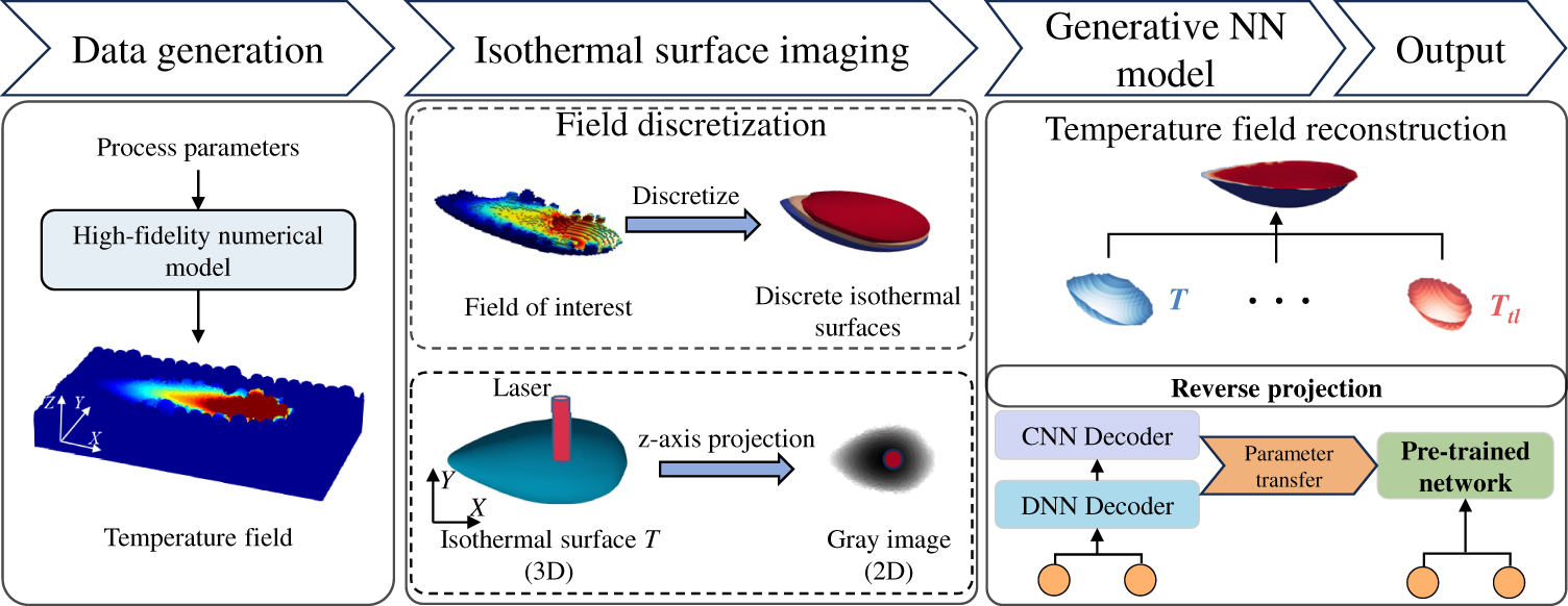
Figure 1: Methodology of the proposed ISI-TL framework for temperature field prediction in metal AM.

2.1 High-Fidelity Thermo-Fluid Flow Model

In this study, the problem of thermo-fluid flow in the LPBF AM is considered. As illustrated in Fig. 2, the primary interfacial phenomena, including heat convection/radiation, heat input, surface tension, and the Marangoni effect, play an important role in the evolution of the temperature field during the scanning process. The governing equations for this problem, including the continuity equation, the momentum conservation equation, and the heat transfer equation, are given below.

{∇⋅u=0ρDuDt=∇⋅(μ∇u)−∇p−K0⋅(1−f)2f3+ε0u+ρg+fv+fsρcpDTDt+Vmetalρmetal LmDfDt=∇⋅(λ∇T)+q(1)

where DϕDt denotes the material derivative of a variable ϕ, u denotes the fluid velocity, ρ denotes the material density, μ denotes the dynamic viscosity, p denotes the pressure, K0 denotes the Carman–Kozeny coefficient of the mushy zone flowing, f denotes the volume fraction of liquid phase, ε0 denotes a small constant to avoid singularity, g denotes the gravity, T denotes the temperature, cp denotes the specific heat capacity, Vmetal denotes the metal volume fraction, Lm denotes the melting latent heat, λ denotes thermal conductivity, q denotes the moving heat source with the given power and scanning speed.

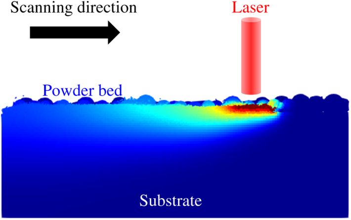
Figure 2: Illustration of the thermo-fluid flow problem in the LPBF AM.

To enhance numerical stability, recoil pressure and surface tension are converted into body force. The recoil pressure fv reads:

fv=ξpp0exp⁡[LVM(T−TV)RTTV]n2ρρmetal +ρgas|∇Vmetal|(2)

where ξp denotes the recoil pressure coefficient, p0 denotes the ambient pressure, LV denotes the latent heat of vaporization, M denotes the molar mass, R denotes the ideal gas constant, TV denotes the vaporization temperature, n denotes the normal vector at the gas/liquid interface.

The surface tension fs including the Marangoni force reads:

fs=(γκn+dγ dT[∇T−(n⋅∇T)n])2ρρmetal +ρgas|∇Vmetal|(3)

with κ being the interface curvature, γ being the surface tension coefficient, and dγ dT being the derivative of surface tension coefficient with respect to temperature.

To accurately simulate the thermo-fluid coupling and transient nonlinear behavior of the molten pool in metal AM, a numerical method that effectively captures free surface evolution and solid-liquid phase change is required. The multiphysics material point method is used in this study. In this method, the material domain is discretized using a set of Lagrangian particles and an Eulerian background grid. The particles carry all material information and track material motion as well as phase interfaces, while the background grid is used to solve the governing equations. In particular, an improved Chorin’s projection method is applied to solve Darcy’s damping, a staggered derivation scheme is applied to calculate surface tension and the Marangoni effect, and a sub-cell occupation technique is introduced for volume fraction treatment. In addition, a semi-implicit local iteration algorithm is adopted for the latent heat calculation. For a detailed description of the multiphysical MPM, please refer to our previous work [20].

2.2 Physics-Guided Isothermal Surface Imaging Method

The physics-guided isothermal surface imaging method is one of the three key components of the ISI-TL framework for reducing the dimensionality of the temperature field. It transforms the prediction of an unstructured, high-dimensional 3D temperature field into a regression problem of a series of structured, low-dimensional 2D grayscale images. Here, the term physics-guided refers to the physically meaningful representation provided by the structured 2D grayscale images, where the learned features correspond to the geometric morphology of isothermal surfaces. Therefore, it consists of two sequential steps: isothermal surface discretization and 2D grayscale image creation. They are detailed as follows.

2.2.1 Isothermal Surface Discretization

The mushy zone is selected as ROI due to its significance in the evolution of material microstructure. Under the assumption of a quasi-steady state of the molten pool, the temperature field within this ROI at the same time is decomposed into distinct isothermal surfaces, as illustrated in Fig. 3.

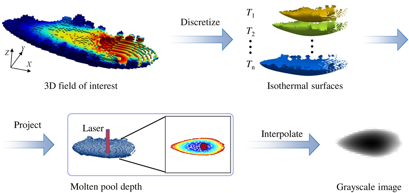
Figure 3: Illustration of the isothermal surface imaging process: from the 3D temperature field of the ROI to 2D grayscale images.

For the isothermal surface STi, the geometric morphology representation is mathematically formalized as a cloud of discrete points XTi(k):

XTi(k)={xj∈R3∣j=1,2,…,nTi(k)}(4)

where the superscript (k) denotes the combination of process parameters, the subscript Ti denotes the temperature value of the isothermal surface, xj∈R3 denotes the spatial coordinate of the j-th discrete point, nTi(k) is the total number of points, which may vary with Ti and k. With the definition of XTi(k), the ROI temperature field can be expressed as a geometric ensemble 𝒟(k):

𝒟(k)={XT1(k),XT2(k),…,XTm(k)}(5)

where m denotes the total number of discrete isothermal surfaces selected for reconstruction.

2.2.2 Grayscale Image of the Isothermal Surface

The discrete isothermal surfaces are converted into corresponding 2D grayscale images. Each 2D grayscale image maintains the same size across all samples, where the pixels represent the coordinates (x, y) of XTi(k). The intensity of each pixel indicates the vertical depth of the isothermal surface relative to a specified z value. This algorithm not only achieves dimensionality reduction but, more importantly, preserves critical physical information. This conversion is essential for the effective application of CNN in the proposed PHPG-NN.

To align all 2D images, we define a local coordinate system. In the LPBF process, the center of the laser beam determines the temperature distribution, especially within the molten pool and the surrounding mushy zone. Therefore, the laser center is designated as the origin of the local coordinates. Let xlaser(k)=(x0(k),y0(k),z0(k)) represent the laser center for the k-th sample. Consequently, for an isothermal surface with a temperature value of Ti, we can rewrite XTi(k) as:

XTi(k)=XTi(k)−xlaser(k)(6)

Likewise, a square domain Ω(k) for the 2D image is centered at (x0(k),y0(k)), namely,

Ω(k)=[−L/2, +L/2]×[−L/2, +L/2](7)

where L is the side length of the domain, which is discretized into a structured mesh of N×N cells. Thus, the subregion of each cell, Cαβ(k), is determined as:

Cαβ(k)=[x0(k)−L/2+αΔ,x0(k)−L/2+(α+1)Δ)×[y0(k)−L/2+βΔ,y0(k)−L/2+(β+1)Δ)(8)

with α,β∈{0,1,…,N−1}, and Δ=L/N the spatial resolution. (As a tradeoff between resolution and computational cost, N is set as 32, and L as 320 µm in this study.) The coordinates of the cell center are calculated as:

gαβ(k)=(−L/2+(α+0.5)Δ,−L/2+(β+0.5)Δ)(9)

The intensity of the pixels for each cell is determined by the distance from its center to the isothermal surface. To this end, a Delaunay triangulation mesh of PTi(k) is constructed based on XTi(k). Let d^(g) be the distance from its center to the isothermal surface. For any cell center, it is determined as gαβ(k)∈Ω(k):

d^(gαβ(k))=∑ν∈𝒯(gαβ(k))λν(gαβ(k))zν(10)

where 𝒯(gαβ(k)) represents the set of three vertices of the Delaunay triangle that covers gαβ(k), zν is the z–component of these vertices, and λν(gαβ(k)) are the corresponding area coordinates. It should be noted that the z0(k) coordinate of the laser center is set as the substrate surface, indicating that we only consider the isothermal surface below the substrate surface to avoid the multi-value attribute in the projection operation. The intensity of the pixels, denoted as ITi(k)∈RN×N, is then obtained by normalized d^(gαβ(k)) to the range [0, 1], as follows:

ITi(k)[α,β]={d^(gαβ(k))−zminzmax−zmin,gαβ(k)∈ℋ(PTi(k))0,otherwise(11)

where zmin and zmax denote the minimum and maximum values of z value among all samples, respectively. ℋ(PTi(k)) is the convex hull of the projected points, defining the valid interpolation region.

2.3 Pre-Trained Hybrid Parameter-to-Image Generative Neural Network

The proposed PHPG-NN is designed to directly map process parameters to the 2D grayscale image of the isothermal surface. It utilizes a hybrid deep learning architecture to achieve low-to-high dimensionality mapping. To effectively reduce overfitting and improve both the convergence speed and generalization capability of the model, a two-stage of pre-training and fine-tuning strategy is implemented for the PHPG-NN. The details of this PHPG-NN are explained as follows.

2.3.1 Architecture of the PHPG-NN

As illustrated in Fig. 4, the proposed architecture comprises two cascaded functional modules. The first module is a parameter embedding module based on fully connected layers, referred to as the DNN module. The other is a surface reconstruction module based on transposed convolutional layers, referred to as the CNN module.

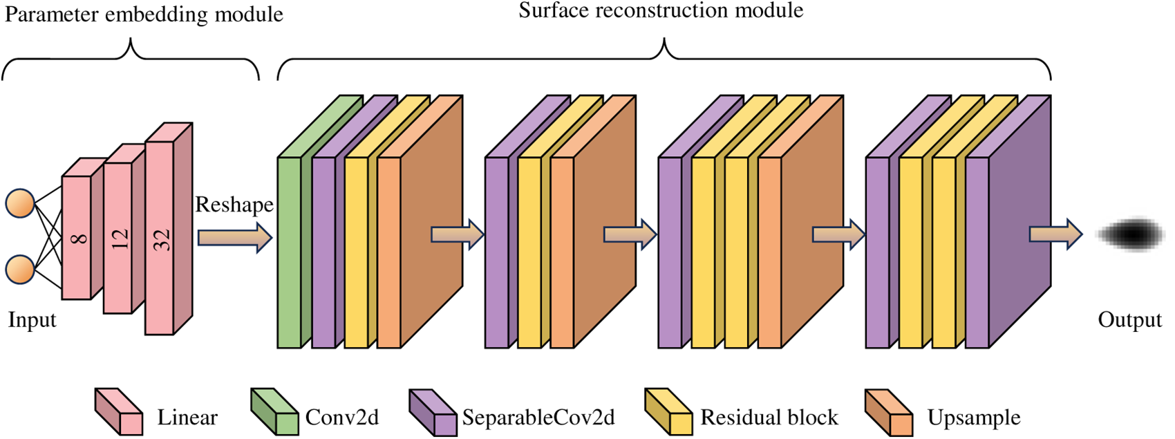
Figure 4: The architecture of the proposed PHPG-NN, showing the information flow from process parameters to the isothermal surface via the DNN and CNN modules.

In the DNN module, a non-linear transformation from the process parameter space to the latent feature space is implemented. It is designed as a fully connected block that takes a vector of process parameters p∈R2 as input. This transformation passes through two sequential hidden layers, which are formulated as:

h1=σ(W1p+b1)h2=σ(W2h1+b2)z=σ(W3h2+b3)(12)

where h1 and h2 denote the intermediate hidden representations, z∈RD denotes the latent feature vector of the output with dimension D, Wi and bi denote the weight matrices and bias vectors for the i-th layer, respectively. σ(⋅) is the non-linear activation function.

The latent vector z is mapped to a structured feature tensor through a reshaping operator ℛ, namely,

Z(0)=ℛ(z)∈RC0×H0×W0,s.t. D=C0×H0×W0(13)

where C0 is the channel dimension, and H0 and W0 denote the height and width corresponding to the initial feature map, respectively. The tensor Z(0) serves as an input for the subsequent CNN module. In this study, the latent feature vector is reshaped into the dimensions of 2×4×4 (i.e., C0=2, H0=4, W0=4).

In the CNN module, depthwise separable convolutions [21] are used to effectively recover the spatial details of the 2D grayscale images from the input of Z(0). This technique factorizes a standard convolutional kernel into two separate operations: one for separate spatial (depthwise) and the other for channel-wise (pointwise) convolutional kernels. This factorization significantly reduces the number of learning parameters. The operation proceeds in two sequential stages. In the first state, spatial filtering is conducted independently on each input channel using depthwise convolution, namely,

Z^c,i,j(ℓ)=∑m=13∑n=13Zc,i+m−2,j+n−2(ℓ)⋅Kc,m,n(ℓ,dw)(14)

where Z(ℓ)∈RCℓ×Hℓ×Wℓ denotes the input feature map in layer ℓ, Z^(ℓ) denotes the intermediate feature map produced by depthwise convolution, the indices (i,j) denote the spatial coordinates of the output feature map, c∈{1,…,Cℓ} denotes the input channel, and K(ℓ,dw)∈RCℓ×3×3 is the depthwise convolutional kernel, where the superscript dw indicates the depthwise operation. Each channel is associated with an independent spatial kernel of size 3×3. Subsequently, the pointwise convolution performs the channel mixing via a 1×1 convolutional kernel to project the intermediate features into a new channel space. This operation constitutes the residual branch transformation, yielding the output feature map as:

Z~c′,i,j(ℓ+1)=∑c=1CℓZ^c,i,j(ℓ)⋅Kc′,c(ℓ,pw)+bc′(ℓ,pw)(15)

where Z~(ℓ+1)∈RCℓ+1×Hℓ×Wℓ denotes the output of the pointwise convolution, c′∈{1,…,Cℓ+1} denotes the output channel, K(ℓ,pw)∈RCℓ+1×Cℓ is the pointwise convolutional kernel, where the superscript pw denotes the pointwise operation, and bc′(ℓ,pw) is the bias term associated with the c′-th output channel.

To facilitate efficient gradient propagation, the module incorporates residual blocks with skip connections. For a given residual unit receiving input feature map Z(ℓ), the output Z(ℓ+1) is calculated as:

Zc′,i,j(ℓ+1)=σ(Z~c′,i,j(ℓ+1))+𝒲(Z(ℓ))c′,i,j(16)

where the operator 𝒲(⋅) denotes a linear projection (typically a 1×1 convolutional kernel) applied to the skip connection, aiming for dimensionality alignment.

2.3.2 Pre-Training and Fine-Tuning of the PHPG-NN

The parameters of PHPG-NN are initialized using the pre-training strategy. As illustrated in Fig. 5, a convolutional autoencoder is trained on augmented grayscale images to learn their latent features. The decoder of this autoencoder provides a high-quality initialization for the CNN module. Furthermore, a latent-variable autoencoder is trained to learn the bidirectional mapping between the process parameters and the latent feature of the images. The decoder of this latent-variable autoencoder offers the initialization for the DNN module. Once initialized, the parameters of the PHPG-NN are further fine-tuned via the supervised training.

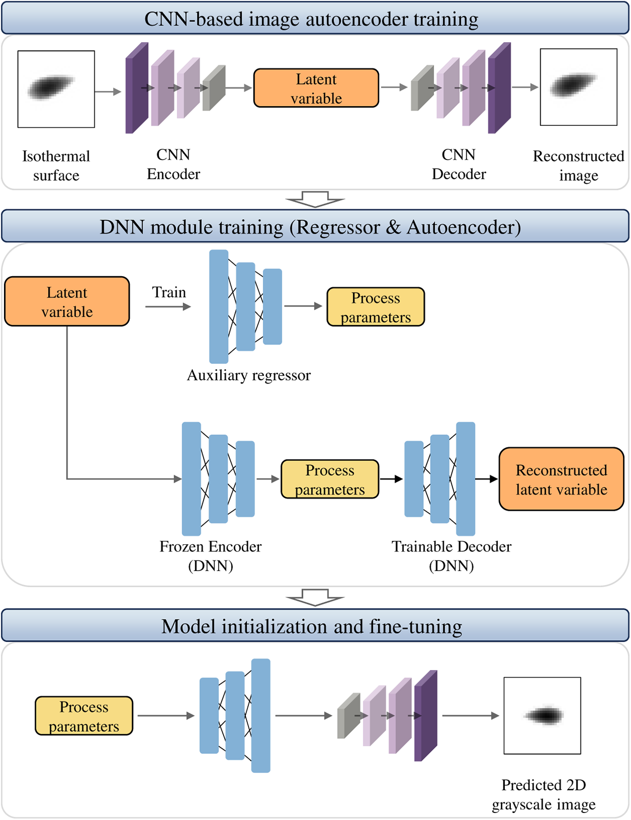
Figure 5: Flow chart of the training and optimization process for the proposed PHPG-NN.

In convolutional autoencoder (CAE) training, data augmentation techniques such as random translation, flipping, and rotation are applied to images. The encoder maps the augmented image to its latent features, expressed as:

ZCAE=fenc(I~;Θenc)(17)

where I~ is the augmented image, ZCAE is the compressed latent variable (the encoder output), and fenc(⋅;Θenc) denotes the convolutional encoder function parameterized by weights Θenc. The decoder reconstructs the image I^ from ZCAE, namely,

I^=fdec(ZCAE;Θdec)(18)

where fdec(⋅;Θdec) is the decoder function parameterized by weights Θdec. The purpose of autoencoder training is to minimize reconstruction loss ℒrec between the augmented image I~ and the reconstructed augmented image I^:

ℒrec(Θenc,Θdec)=1Ntrain∑i=1NtrainL(I~i,I^i)(19)

with L(⋅,⋅) being the mean squared error (MSE) and Ntrain being the number of training samples.

The latent variable autoencoder is trained to link parameters p to the latent variables ZCAE. To this end, an auxiliary regressor is first trained with ZCAE as input to predict the corresponding process parameters p, as follows:

p=henc(ZCAE;Φenc)(20)

where henc(⋅;Φenc) denotes the encoder mapping function parameterized by Φenc. Upon convergence, the parameters of this component Φenc are frozen. Subsequently, to establish the forward mapping from process parameters to latent variables, a symmetric mapping module in the form of an autoencoder is employed to reconstruct the latent features, as shown in Fig. 5. It is expressed as:

Z^CAE=hdec(henc(ZCAE;Φenc);Φdec)(21)

with hdec(⋅;Φdec) being the decoder mapping function that reconstructs latent variables from the process parameters. The model parameters Φdec are optimized by minimizing the latent reconstruction loss of ‖ZCAE−Z^CAE‖22.

Finally, well-optimized Φdec and Θdec are assigned to the DNN and CNN part defined in Section 2.3.1. The initialized PHPG-NN is expressed as:

I^gen=fdec(hdec(p;Φdec);Θdec)(22)

where I^gen is the grayscale image generated according to a given set of process parameters. During the fine-tuning process, the parameters of the CNN module (Θdec) remain frozen, and the parameters of the DNN module (Φdec) are optimized to minimize:

Φ=arg⁡minΦE(p,I)‖I−fdec(hdec(p;Φ);Θdec)‖2(23)

with Φ being the trainable parameters for the function hdec, I being the ground truth, and E(p,I) being the expectation over the loss distribution. Once a 2D grayscale image is predicted with the well-trained PHPG-NN, the corresponding isothermal surface can be obtained by the reverse operation of the isothermal surface imaging algorithm in Section 2.2.

2.4 Transfer Learning Strategy

The PHPG-NN model, which is trained on an isothermal surface, can be further adapted to predict other isothermal surfaces at different temperatures through transfer learning. The original PHPG-NN model is referred to as the parent PGPG-NN, while its adaptations are called the transferred PHPG-NN. Let ℐ={IT1,IT2,…,ITK} represent a set of target isothermal surfaces of the ROI. Here, ITK∈RN×N corresponds to the isothermal surface at a specific temperature Tk. Since these isothermal surfaces are governed by the same physical laws (heat transfer, fluid dynamics), they share high geometric feature similarity, providing a solid physical foundation for applying transfer learning.

The transfer learning procedure begins with a well-trained parent PHPG-NN, denoted as 𝒩base. The parameters of it are represented as {Φbase,Θbase} (corresponding to Φdec and Θdec, as derived in Section 2.3). For each subsequent target isothermal surface ITk, the parameters {Φk,Θk} of the k-th transferred PHPG-NN are initialized as:

Φk(0)=Φbase,Θk=Θbase(24)

We assume that the CNN module has learned to extract general geometric features of isothermal surfaces, while the DNN module needs to learn the specific mapping between these features and the process parameters for different temperatures. Therefore, a fine-tuning strategy is applied to optimize Φk(0), while Θk is frozen, allowing low-cost extension to predict new isothermal surfaces. The optimization objective for the k-th isothermal surface is formulated to find the optimal mapping parameters Φk∗ by minimizing the prediction error:

Φk∗=arg⁡minΦk(0)E(p,ITk)‖ITk−fdec(hdec(p;Φk(0));Θbase)‖2(25)

This transfer learning is carried out iteratively for all target temperature values. Once completed, a set of transferred PHPG-NNs {𝒩T1,𝒩T2,…,𝒩TK} is created. For a specific set of process parameters ptest, these transferred PHPG-NNs can generate predictions {I^T1,I^T2,…,I^TK} in parallel. Since all transferred PHPG-NNs are fine-tuned with isothermal surfaces spatially normalized to the laser center position (as defined in Section 2.2), the predicted isothermal surfaces for any given process parameters share the same laser-centric coordinate system. This alignment ensures that the surfaces are consistently positioned in 3D space. Finally, a 3D temperature field can be reconstructed based on ℐ, where a linear interpolation is conducted between adjacent isothermal surfaces.

2.5 Overall Implementation Procedure

The overall implementation procedure of the proposed ISI-TL framework is summarized below.

1.    Generate samples using the high-fidelity thermo-fluid flow solver described in Section 2.1 for different combinations of process parameters p(k)=(Pk,Vk).

2.    Extract isothermal surfaces from each simulation data and create the samples of 2D grayscale images through the physics-guided isothermal surface imaging algorithm detailed in Section 2.2.

3.    Train a partent PHPG-NN 𝒩base for a selected isothermal surface using the training strategy described in Section 2.3.

4.    Obtain a set of transferred PHPG-NNs for other isothermal surfaces using the transfer learning strategy presented in Section 2.4.

5.    For a new set of process parameters ptest, predict all target isothermal surfaces {I^T1,I^T2,…,I^TK} using the parent and the transferred PHPG-NNs.

6.    Reconstruct the 3D temperature field based on {I^T1,I^T2,…,I^TK}, taking advantage of the intrinsic spatial alignment of the laser-centric coordinate system and the linear interpolation.

3  Results and Discussion

This section presents a thorough evaluation of the proposed ISI-TL framework against the high-fidelity simulation results using multiphysics MPM in Section 2.1. First, we discuss hyperparameter optimization to identify the optimal network architecture within a predefined search space. Second, the performance of PHPG-NN is evaluated for a specific isothermal surface. Finally, the 3D temperature field is reconstructed from the predicted isothermal surfaces using the transfer learning strategy.

In this study, all networks were developed with PyTorch 1.10.2 (Python 3.8.12). The architecture features the Swish activation function [22] and uses 3×3 kernels for spatial convolutions and 1×1 kernels for pointwise operations. The weights were initialized using the He method [23] for convolutional layers and standard random initialization for fully connected layers. Training was optimized using the AdamW optimizer [24] with default parameters, while learning rates and epochs were tuned specifically for each model’s configuration. All numerical simulations were conducted on an Intel Xeon E5-2680 supercomputer platform, while PHPG-NN training and prediction were performed on a workstation equipped with an NVIDIA GeForce RTX 2070 SUPER GPU.

The structural similarity index (SSIM), the normalized root mean square error (NRMSE), and the coefficient of determination (R2) are used to quantitatively assess perceptual fidelity, error magnitude, and explained variance, respectively. SSIM evaluates the structural consistency between the ground truth and the predicted images, defined as:

SSIM(I,I^gen)=(2μIμI^gen+c1)(2σII^gen+c2)(μI2+μI^gen2+c1)(σI2+σI^gen2+c2)(26)

where μI and μI^gen represent the mean value of the ground truth and the reconstructed image, respectively; σI2 and σI^gen2 represent the variances of the ground truth and the prediction, respectively; σII^gen is the covariance between ground truth and prediction, and c1=0.012 and c2=0.032 are stability constants. NRMSE quantifies the global reconstruction discrepancy, normalized by the range of the corresponding grayscale image. It reads:

NRMSE(I,I^gen)=N−1||I−I^gen||Fmax(I)−min(I)(27)

where ‖⋅‖F denotes the Frobenius norm. R2 measures the proportion of spatial variance explained by the model, expressed as:

R2(I,I^gen)=1−||I−I^gen||F2||I−μI||F2(28)

3.1 Data Set Generation

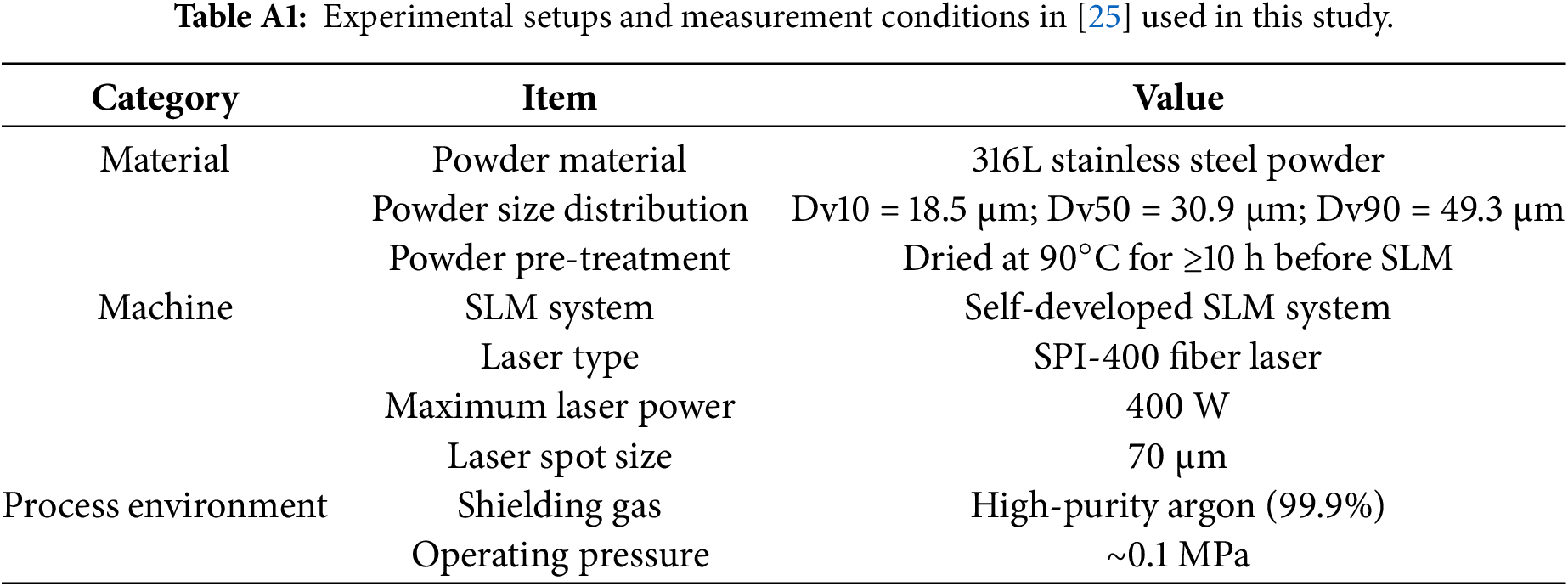
A single-track deposition process in the LPBF is studied under different combinations of laser power and scanning speed. To generate the training samples, the high-fidelity numerical model based on multiphysics MPM is used. The accuracy of this numerical model is validated against the experimental data [25]. Details of the experimental setups, including the specific machine and measurement techniques, are provided in Table A1. In the experiment, the process parameters include a laser power of 200 W, a scanning speed of 800 mm/s, a beam diameter of 70 µm, and an absorption coefficient of 0.38. A powder layer with an average particle diameter and layer thickness of 30 µm was deposited on a stainless steel substrate. The material properties of the 316 L stainless steel used in the simulation are listed in Table A2.

The simulation was conducted with a domain size of 0.6 mm×0.3 mm×0.18 mm and a cell size of 4 µm, corresponding to a particle spacing of 2 µm. The physical time and the time step were set to 7.5×10−4 s and 1×10−7 s, respectively. It should be noted that only the melt pool width can be obtained from the experimental measurement in Reference [25]; no experimental data on the melt pool length and depth are available. To fully demonstrate the accuracy of the MPM model, we conducted an additional numerical simulation using the FVM with high mesh resolution. The numerical results from the MPM model are quantitatively compared with the experimental data as well as those obtained from the FVM in Table 1. Regarding the width of the molten pool, both numerical results agree well with the experimental data, with a relative error of 3.70% for the multiphysics MPM result, which is smaller than that of the FVM result. In terms of the length and depth of the molten pool, both numerical results are in good agreement with each other, where the experimental data is absent due to the lack of corresponding measurements. It is worth noting that the molten pool depth predicted by the multiphysics MPM is lower than that by the FVM, which is reasonable because the molten pool width is larger in the former than in the latter. In addition, the accuracy of the Multiphysics MPM on the LPBF problem has been fully demonstrated in our previous study [20]. All in all, the accuracy of the MPM model in this study is reasonably validated, and it is used to generate a reliable data set.

The parameter space is set to the LPBF processing window to ensure a stable molten pool, as observed experimentally. For the manufacturing system utilized by Yuan et al. [25], it was identified that a scan speed below 800 mm/s with the laser power fixed at 200 W can yield highly uniform and continuous melt tracks, whereas higher scan speeds may lead to necking or even balling defects. Therefore, 800 mm/s is adopted as the upper bound of the scan speed range to reduce the complexity of the numerical simulations.

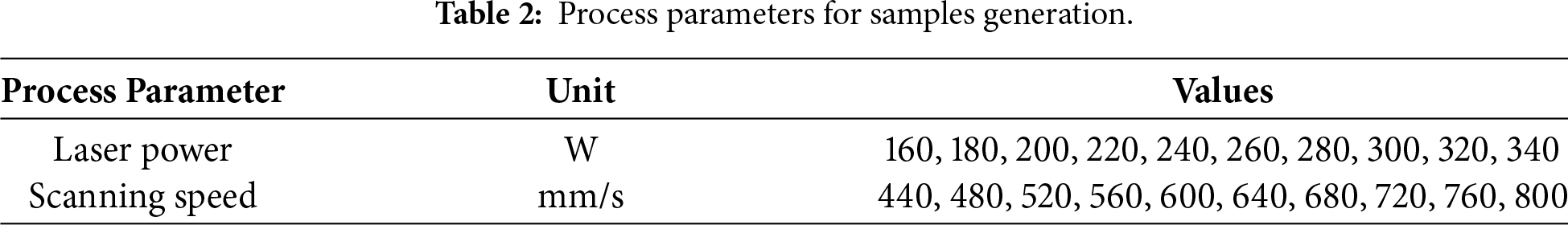
Based on the selected variables and the defined parameter range, a full factorial design of experiments was constructed with the ranges of P and V listed in Table 2. It results in 100 cases with unique combinations of process parameters, which were simulated by the validated numerical model using MPM. The resulting samples have the process parameters (P, V) as input and their corresponding temperature fields as output, which serve as the foundation for PHPG-NN training and validation.

Although the proposed framework takes two process parameters as input, it is straightforward to add more process parameters, but at the expense of more training samples and more sophisticated training strategies. Additional variables can be incorporated by either extending the input variable set or through composite descriptors derived from multiple process parameters. In this scenario, the mapping is defined in a higher-dimensional process space, thereby increasing the problem’s complexity. Consequently, more representative training data, greater model capacity, and careful training are required to maintain stable convergence. From the perspective of transfer learning, the proposed framework retains most of its advantages, as it leverages reusable feature representations learned from predicting one set of isothermal surfaces to accelerate learning on related isothermal surface tasks. However, introducing additional parameters requires greater network capacity along with retraining and fine-tuning to accommodate stronger nonlinearities and parameter couplings introduced by the higher-dimensional input.

3.2 Network Architecture and Hyperparameter Analysis

This section provides a systematic study of hyperparameter effects on PHPG-NN performance. Using a controlled-variable approach, we evaluate each hyperparameter sequentially while keeping all other settings fixed.

3.2.1 Hyperparameters for the Convolutional Autoencoder

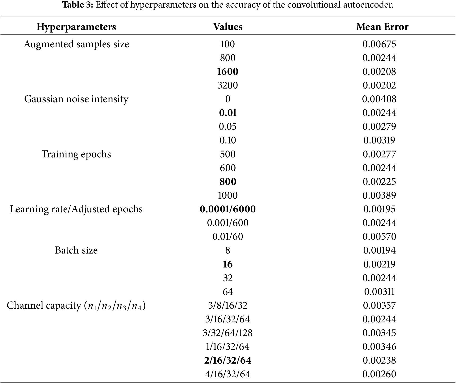
The hyperparameters of the convolutional autoencoder include six critical factors. They are augmented sample size, Gaussian noise intensity for latent space, training epochs, learning rate, batch size, and channel capacity. The mean reconstruction errors for all cases are compared in Table 3. This comparison reveals that the mean reconstruction error consistently decreases as the augmented sample size increases. The effect of Gaussian noise intensity in the latent space on the mean error shows a non-monotonic trend: an appropriate noise intensity effectively enhances model robustness and reconstruction accuracy, while excessive perturbation degrades the performance of the convolutional autoencoder. The number of training epochs is found to be in an optimal range, with the mean error first decreasing and then increasing as training epoch increases. Regarding optimization, it is observed that the mean error increases with the learning rate, where, to ensure a fair comparison, the training epochs are adjusted inversely proportional to the learning rate (e.g., reduced to 60 epochs for the learning rate of 0.01). Within the range of batch sizes, the mean error decreases as the batch size decreases. The channel capacity configuration is represented as n1/n2/n3/n4 for the decoder and n4/n3/n2/n1 for the encoder. Among the given configurations, 2/16/32/64 yields the lowest mean reconstruction error. The corresponding training and validation loss curves, as well as the reconstruction results of the test samples, are presented in Fig. A1. Based on these comparisons, the values highlighted in bold for the hyperparameters listed in Table 3 were selected for this study to well balance computational cost and prediction accuracy.

3.2.2 Hyperparameters for the DNN Autoencoder

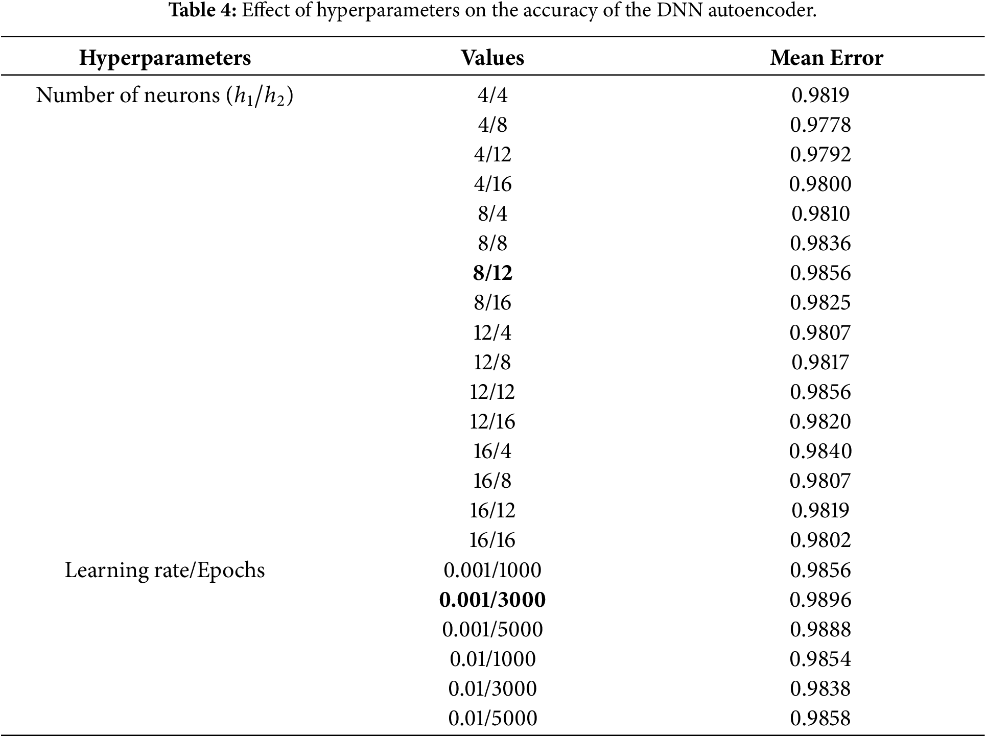
The hyperparameters considered for the DNN autoencoder include three critical factors. They are the number of neurons per hidden layer, the learning rate, and the number of training epochs. The ranges of these hyperparameters are summarized in Table 4, where “h1/h2” indicates the number of neurons in the two hidden layers, which can take values of 4, 8, 12, or 16. The training and validation loss curves, along with the reconstruction results of the test samples, are presented in Fig. A2. Based on these comparisons, the values highlighted in bold in Table 4 were selected for the corresponding hyperparameters in this study to well balance computational cost and prediction accuracy.

3.3 Prediction of a Single Isothermal Surface by PHPG-NN

For fine-tuning and testing, isothermal surfaces at 1658 K are used from the 100 samples. With these samples, 60% is used for training and validation (50 samples for fine-tuning and 10 samples for validation), while the remaining data (40 samples) is used for testing the PHPG-NN. In the test samples, 20 samples have process parameters outside the convex hull of the training parameter space. During fine-tuning, a learning rate of 1×10−5 is used with 80 epochs. The loss profiles are plotted in Fig. 6, indicating a well-trained PHPG-NN for the prediction of the specific isothermal surface.

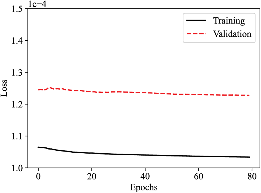
Figure 6: Training and validation loss profiles during the fine-tuning process.

The performance of PHPG-NN in terms of SSIM, NRMSE, and R2 on the test samples is summarized in Table 5. The average SSIM is 0.986, the NRMSE is 0.025, and the R2 is 0.990, indicating the high accuracy of the proposed PHPG-NN. Moreover, a comparison of the grayscale images between the ground truth and the NN model’s predictions is shown in Fig. 7. They are in good agreement across different combinations of the process parameters. As indicated by the absolute error map, the differences exist mainly along the boundary of the isothermal surface projection. Fig. 8 further compares the reconstructed isothermal surface from the predicted grayscale image with the ground truth. Good agreements are achieved, with an average error of approximately 2% with respect to the maximum depth of the molten pool.

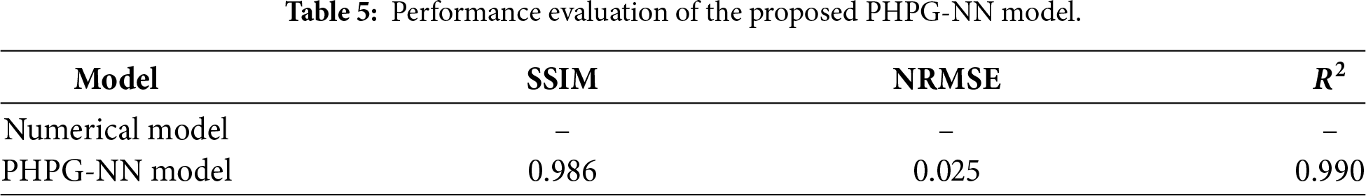
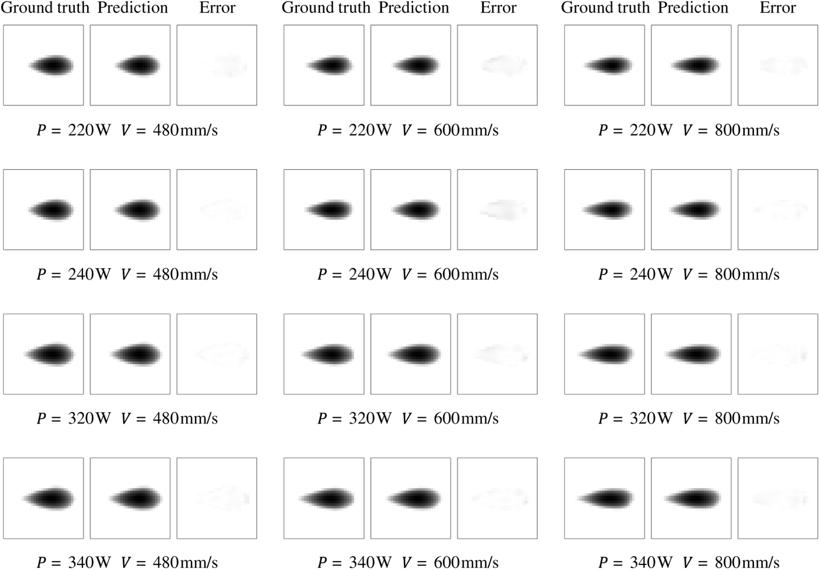
Figure 7: Comparison of the grayscale images from the PHPG-NN and numerical simulations for the given process parameters, where the absolute error map shows the distribution of the difference between the two images.

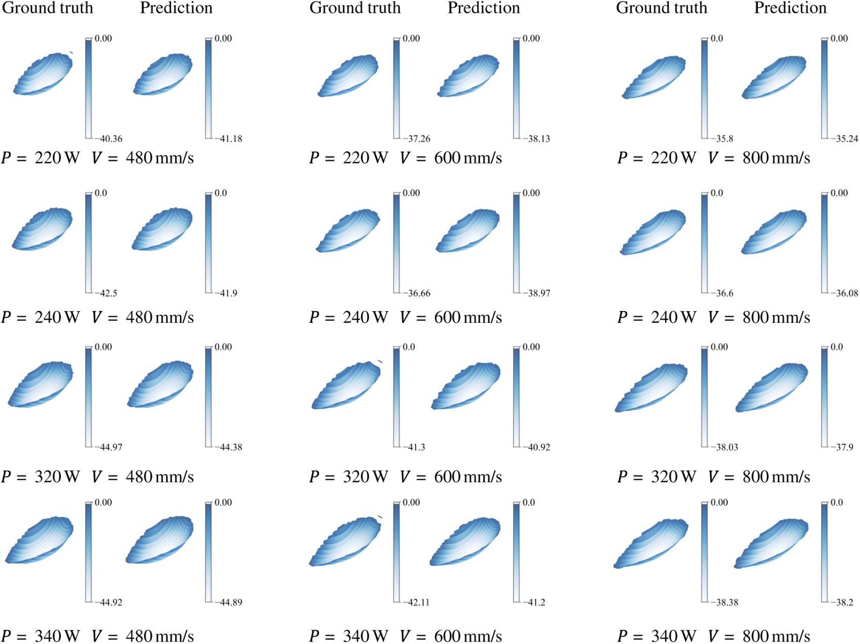
Figure 8: Comparison of the reconstructed isothermal surfaces from the PHPG-NN and numerical simulations for the given process parameters.

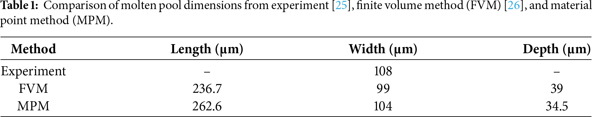
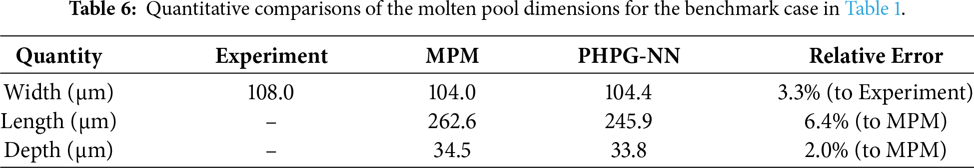
In addition, the comparison between the predicted molten pool dimensions and the benchmark results in Table 1 is summarized in Table 6 to demonstrate the experimental consistency of the PHPG-NN prediction. For the molten pool width, the relative error of the PHPG-NN prediction to the experimental result is 3.3%. Since the molten pool length and depth are not available experimentally, the results from the MPM model are used as the reference solution. The predicted molten pool length of 245.9 µm is close to the MPM result of 262.6 µm, with a difference of 6.4%, while the predicted depth of 33.8 µm is close to the MPM result of 34.5 µm, with a difference of 2.0%. The molten pool dimensions from the PHPG-NN are shown to conform to physically meaningful geometry, thereby validating the predictive fidelity of the proposed model.

3.4 3D Temperature Field Reconstruction Based on Transfer Learning

In this section, the PHPG-NN trained for the 1658 K-isothermal surface is extended to first predict the 1723 K-isothermal surface, and then the isothermal surfaces with temperature values of 1684, 1700 and 1712 K to construct the 3D temperature field of the ROI. For fine-tuning during transfer learning, a learning rate of 1×10−3 is used.

The evolution of the training and the validation loss for the isothermal surface at 1723 K, using 50 samples for the training, is shown in Fig. 9. Both curves exhibit rapid decay during the first 50 epochs and achieve stable convergence after approximately 200 epochs, which highlight the efficiency of the transfer learning. Furthermore, Table 7 lists the average SSIM of 0.9832, the NRMSE of 0.0369, and the R2 of 0.9865 across the 40 test samples. These results demonstrate that the transferred PHPG-NN achieves high accuracy. Fig. 10 compares the predictions from the transferred PHPG-NN and the high-fidelity numerical model in terms of grayscale image for six test samples. They are in good agreement, with absolute errors mainly occurring along the boundaries of the isothermal surface projection. The corresponding isothermal surfaces reconstructed from the predicted grayscale images are shown in Fig. 11, and they are in line with the ground truth provided by the high-fidelity numerical model. Furthermore, the effect of the number of training samples on the prediction accuracy is examined. As shown in Table 7, a gradual reduction in the number of training samples results in a slight decline in the accuracy of the test samples. In particular, even with 20 samples, the transferred PHPG-NN maintains competitive performance, achieving an average R2 of 0.9858, an average SSIM of 0.9821, and an average NRMSE of 0.0373. This highlights the effectiveness of the transfer learning applied to the PHPG-NN.

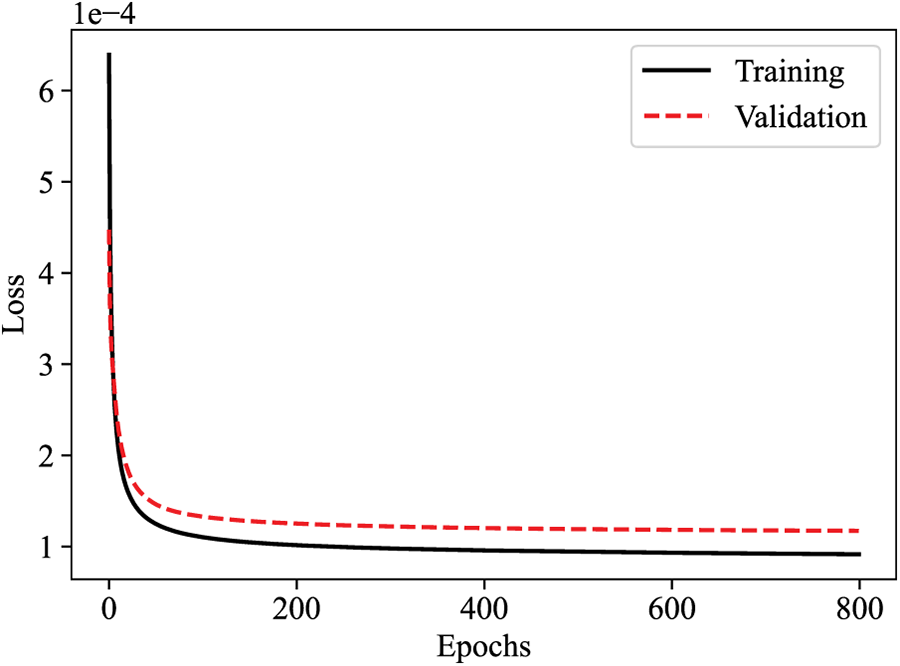
Figure 9: Training and validation loss profiles during the fine-tuning of the transferred PHPG-NN.

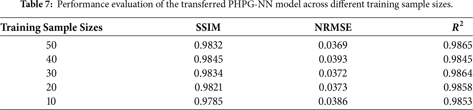
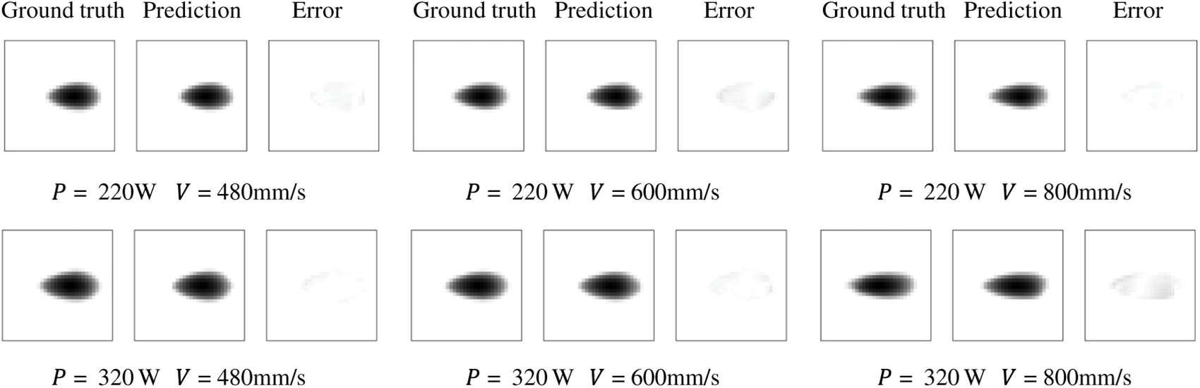
Figure 10: Comparison of the grayscale images from the transferred PHPG-NN and numerical simulations for the given process parameters, where the absolute error map shows the distribution of the difference between the two images.

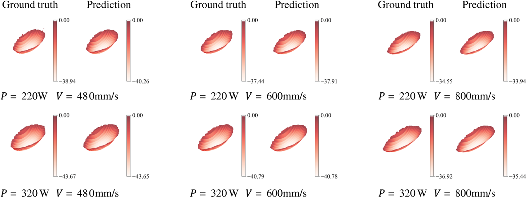
Figure 11: Comparison of the reconstructed isothermal surfaces from the transferred PHPG-NN and numerical simulations for the given process parameters.

A 3D temperature field is reconstructed using a series of PHPG-NNs and the spatial interpolation algorithm. The PHPG-NNs include the one trained with 50 samples and the ones based on transfer learning. Five isothermal surfaces at temperatures 1658, 1684, 1700, 1712 and 1723 K are predicted for test cases with different process parameters. It should be noted that, because the temperature gradient is very high and there are prediction errors, the adjacent isothermal surfaces may exhibit non-physical penetration at some spatial points. It further leads to spatial interpolation errors for the scenario where the spacing between neighboring isothermal surfaces in high gradient regions is smaller than the grid cell spacing. As a consequence, small prediction errors may lead to local disordering. To ensure thermodynamic consistency, we first locate the nodes that exhibit local penetration, then iteratively adjust their positions along the temperature gradient. The 3D temperature fields reconstructed from the five isothermal surfaces, obtained by spatial interpolation, are plotted in Fig. 12, along with their counterparts from the high-fidelity numerical model for comparison. Both results are found in good agreement, demonstrating the accuracy and effectiveness of the proposed framework.

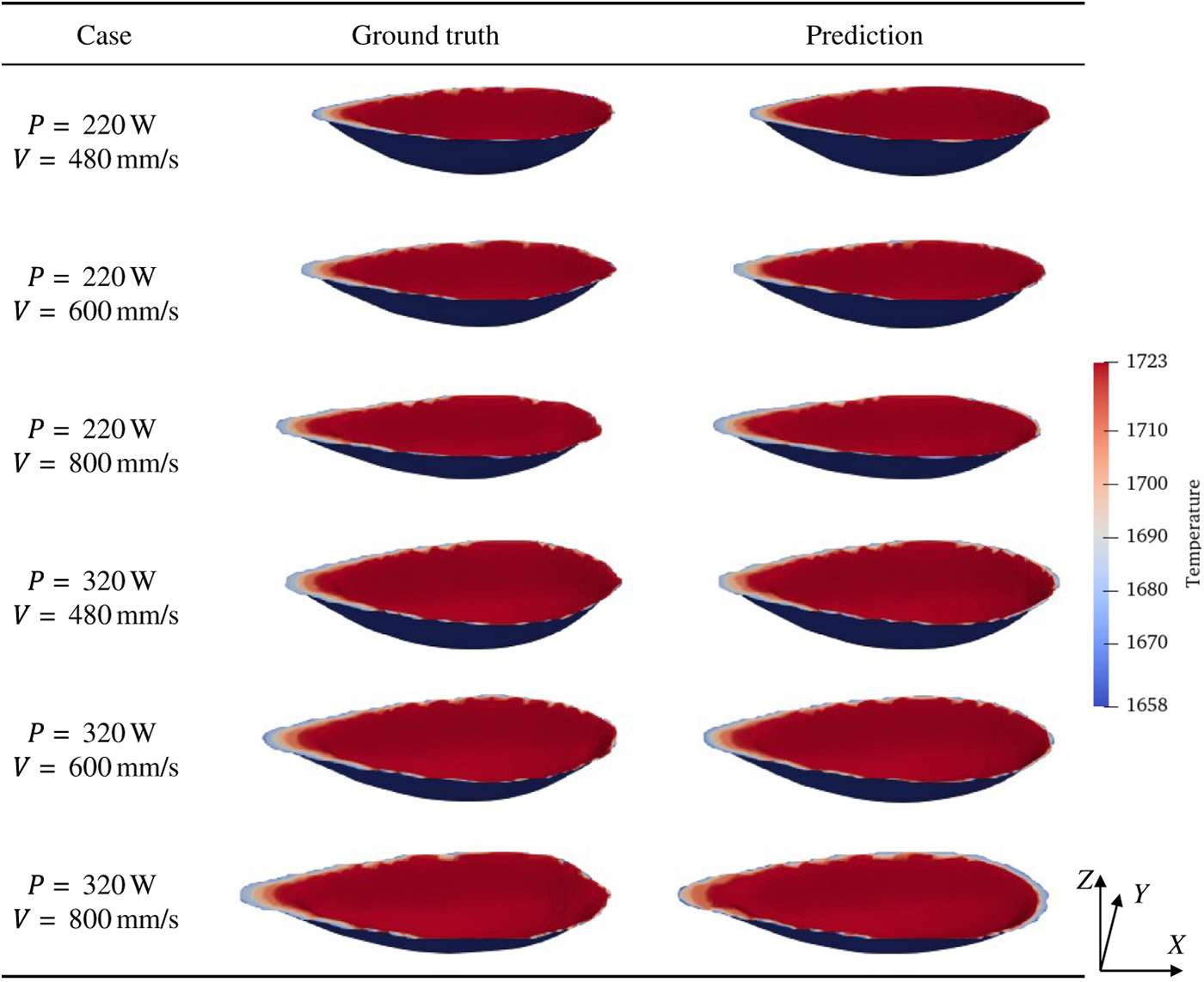
Figure 12: Comparison of temperature field within the ROI between the ISI-TL framework and the high-fidelity numerical models.

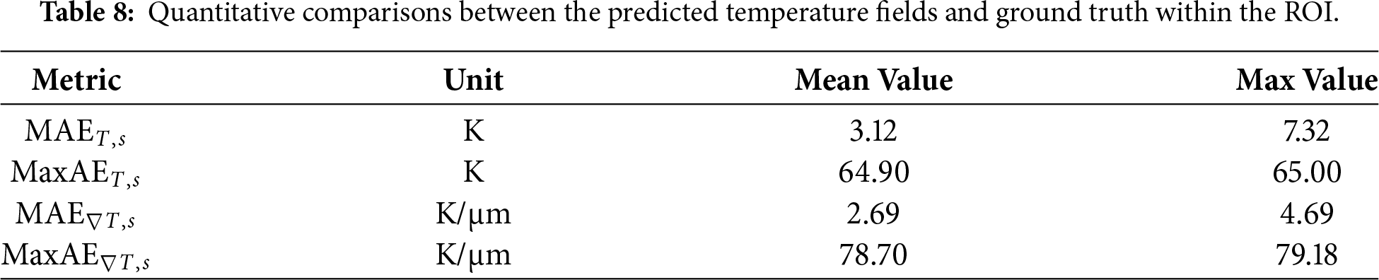
Furthermore, the quantitative comparisons are summarized in Table 8. Let MAET,s and MaxAET,s denote the mean and maximum voxel-wise absolute temperature errors evaluated within the ROI of each individual sample s, respectively. Likewise, MAE∇T,s and MaxAE∇T,s are defined as the voxel-wise temperature gradient difference within each sample s. The mean and maximum values are obtained by further aggregating these sample-wise metrics across all test samples. Within the ROI, the mean values of MAET,s and MaxAET,s are 3.12 and 64.90 K, and their maximum values across test samples are 7.32 and 65.00 K, respectively. For temperature gradients, the mean values of MAE∇T,s and MaxAE∇T,s are 2.69 and 78.70 K/µm, and their maximum values are 4.69 and 79.18 K/µm, respectively.

The non-physical penetration behavior is further quantified, and its frequency is summarized in Table 9. For the the interpolation samples, the penetration frequency ranges from 0.0031 to 0.0618 with a mean value of 0.0194 and a variance of 3.03×10−4, indicating that adjacent isothermal surfaces exhibit good monotonicity over most regions of the training domain. For the extrapolation samples, the penetration frequency increases to the range of 0.1218 to 0.2688 with a mean value of 0.2074 and a variance of 2.36×10−3, indicating both a larger magnitude and greater variability outside the training range.

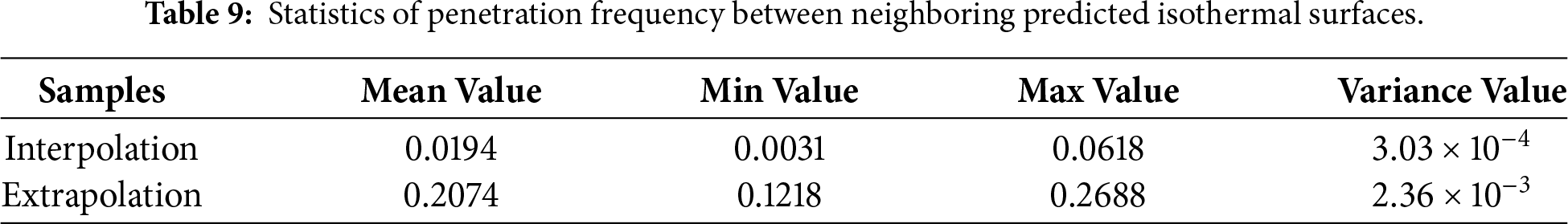
Although the post-processing correction works, it lacks physical consistency. To avoid post-processing corrections, two potential improvements to the current model will be addressed in the future. First, a regularization term that penalizes intersections between adjacent temperature levels can be introduced to the transfer learning to ensure physical consistency. This would avoid local ordering reversal during fine-tuning. Second, multiple isothermal surfaces can be jointly predicted within a unified model, thereby enforcing monotonicity across temperature levels during training and eliminating the need for corrections afterward.

3.5 Computational Efficiency

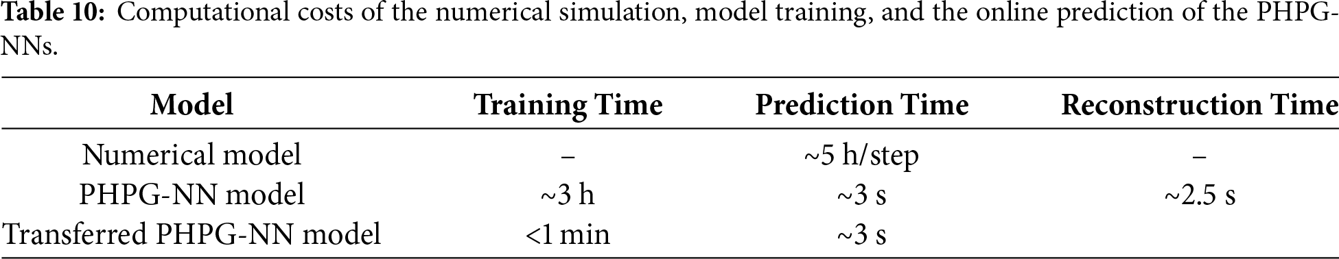
The computational costs of the numerical simulation, model training, and online prediction are summarized in Table 10. The PHPG-NN takes approximately 3 h for offline training and about 3 s to predict a single isothermal surface online. Based on a parent PHPG-NN, the transfer learning takes only 1 min while maintaining comparable prediction accuracy. Generating a 3D temperature field in the ROI takes approximately 3 s using the transferred PHPG-NNs to predict the required isothermal surfaces. Based on the predicted isothermal surfaces, the subsequent reconstruction to obtain one 3D temperature field takes approximately 2.5 s. Therefore, the end-to-end online cost for generating one 3D temperature field is approximately 5.5 s. Once well trained, it enables near real-time prediction and reconstruction. In contrast, the numerical model takes about 5 h for one output interval.

4  Conclusion

In this study, an isothermal surface imaging and transfer learning (ISI-TL) framework is proposed to fast predict isothermal surfaces and to reconstruct the 3D temperature field in metal additive manufacturing. To overcome the challenges of high dimensionality and scarce high-fidelity data, the framework integrates a physics-guided isothermal surface imaging method that encodes the 3D temperature field into structured 2D grayscale images, a pre-trained hybrid parameter-to-image generative neural network (PHPG-NN) that efficiently learns the mapping from process parameters to these isothermal surface images through a two-stage autoencoder initialization strategy, and a transfer learning strategy that leverages the geometric similarity across isothermal surfaces, enabling rapid model adaptation to new temperatures. A high-fidelity numerical model based on the multiphysics material point method is used to generate 100 samples for training and validation. Comprehensive evaluations demonstrate that the ISI-TL framework achieves high predictive accuracy while providing results in seconds. This capability enables near real-time temperature field prediction and reconstruction, offering a high efficient surrogate model for process analysis and optimization.

Despite the advantages of the proposed framework, two limitations need to be addressed in future research. First, the current framework is limited to predict the temperature field at a quasi-steady state. A critical extension would be to predict the full spatiotemporal evolution of the temperature field throughout the scanning process. Second, the physics-guided isothermal surface imaging method cannot handle an isothermal surface with concave feature in the scanning direction, which requires a specialized design for the imaging method. In addition, developing cascaded NN models to connect predicted temperature fields with microstructure and defect formation represents an important research direction toward achieving a comprehensive digital twin of metal additive manufacturing.

In conclusion, the ISI-TL framework and the PHPG-NN model represent a significant step forward in physics-aware, data-efficient surrogate modeling for computational mechanics. By creatively reformulating the field-prediction problem and leveraging transfer learning, this work provides a practical and scalable tool for real-time analysis of complex additive manufacturing processes.

Acknowledgement: The support from the National Natural Science of Foundation of China and the Fundamental Research Funds for the Central Universities to the second author are gratefully acknowledged.

Funding Statement: This research was funded by the National Natural Science Foundation of China under Grant No. 11972086, and the Fundamental Research Funds for the Central Universities.

Author Contributions: The authors confirm contribution to the paper as follows: Conceptualization, Yanping Lian; methodology, Yanping Lian; software, Zhidong Wang and Jiawei Chen; validation, Zhidong Wang; formal analysis, Zhidong Wang and Jiawei Chen; investigation, Zhidong Wang; data curation, Jiawei Chen and Yanping Lian; writing—original draft preparation, Zhidong Wang and Yanping Lian; writing—review and editing, Mingjian Li and Ruxin Gao; visualization, Zhidong Wang; supervision, Yanping Lian; project administration, Yanping Lian; funding acquisition, Yanping Lian. All authors reviewed and approved the final version of the manuscript.

Availability of Data and Materials: The data that support the findings of this study are available from the Corresponding Author, upon reasonable request.

Ethics Approval: Not applicable.

Conflicts of Interest: The authors declare no conflicts of interest.

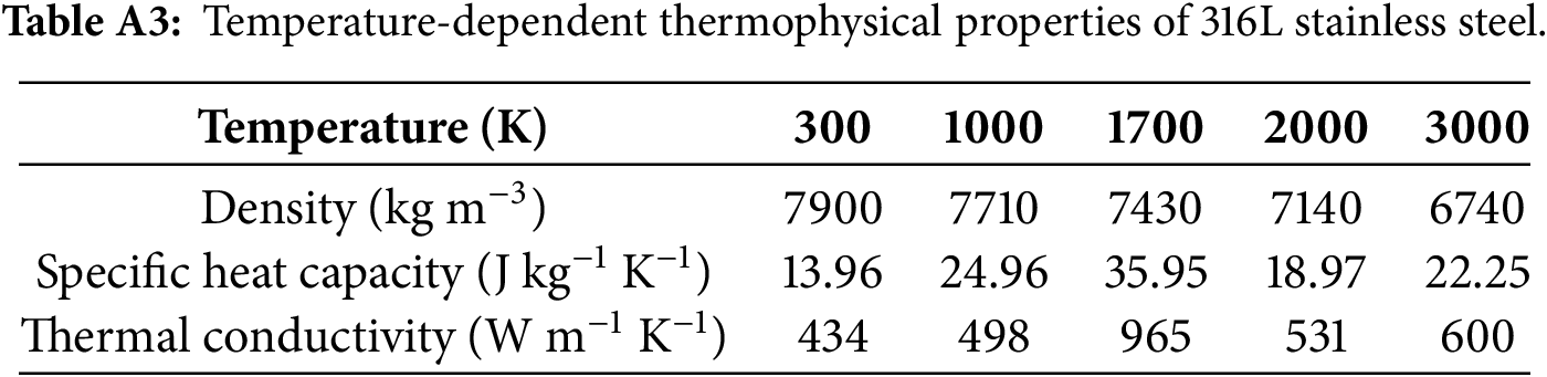
Appendix A Material Properties

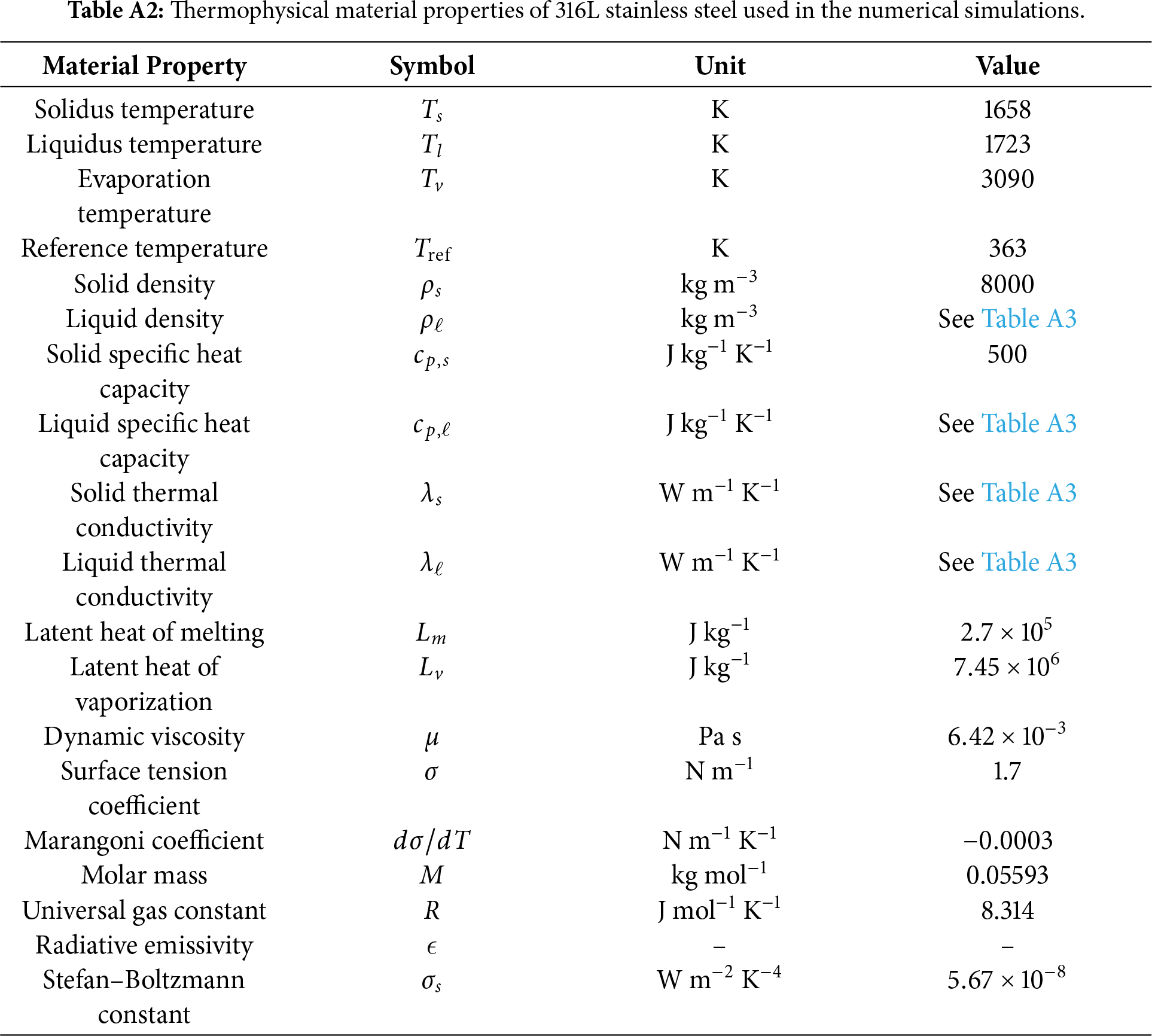
This appendix summarizes the experimental conditions [25] and material parameters used in the numerical simulations. Table A1 summarizes the experimental setups and measurement conditions; Table A2 lists the input thermophysical constants for 316L stainless steel; and Table A3 presents the temperature-dependent properties.

Appendix B Performance Evaluation of the Pre-Training Phase

The performance of the two pre-trained models is evaluated in terms of convergence stability and reconstruction accuracy. The results are summarized in Figs. A1 and A2. The left column illustrates the training and validation loss curves, indicating the optimization process over epochs. The right column presents the corresponding testing results: (1) the distribution of prediction errors; (2) the prediction accuracy of the process parameters; and (3) the reconstruction fidelity of the latent variables.

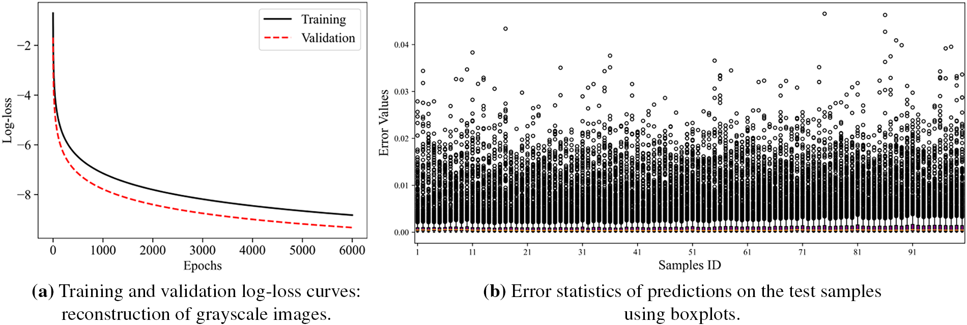
Figure A1: The training and testing performance of the CNN-based autoencoder.

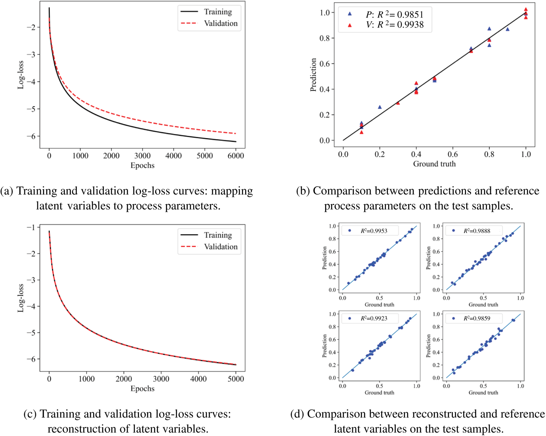
Figure A2: The training and testing performance of the DNN-based autoencoder.

References

1. Pauly S, Wang P, Kühn U, Kosiba K. Experimental determination of cooling rates in selectively laser-melted eutectic Al-33Cu. Addit Manuf. 2018;22:753–7. doi:10.1016/j.addma.2018.05.034. [Google Scholar] [CrossRef]

2. Panwisawas C, Tang YT, Reed RC. Metal 3D printing as a disruptive technology for superalloys. Nat Commun. 2020;11:2327. doi:10.1038/s41467-020-16188-7. [Google Scholar] [PubMed] [CrossRef]

3. Kanishka K, Acherjee B. Revolutionizing manufacturing: a comprehensive overview of additive manufacturing processes, materials, developments, and challenges. J Manuf Process. 2023;107:574–619. doi:10.1016/j.jmapro.2023.10.024. [Google Scholar] [CrossRef]

4. Li Y, Gu D. Thermal behavior during selective laser melting of commercially pure titanium powder: numerical simulation and experimental study. Addit Manuf. 2014;1–4:99–109. doi:10.1016/j.addma.2014.09.001. [Google Scholar] [CrossRef]

5. Le TN, Lo YL. Effects of sulfur concentration and Marangoni convection on melt-pool formation in transition mode of selective laser melting process. Mater Des. 2019;179:107866. doi:10.1016/j.matdes.2019.107866. [Google Scholar] [CrossRef]

6. Tang C, Le KQ, Wong CH. Physics of humping formation in laser powder bed fusion. Int J Heat Mass Transf. 2020;149:119172. doi:10.1016/j.ijheatmasstransfer.2019.119172. [Google Scholar] [CrossRef]

7. Zhu Q, Liu Z, Yan J. Machine learning for metal additive manufacturing: predicting temperature and melt pool fluid dynamics using physics-informed neural networks. Comput Mech. 2021;67(2):619–35. doi:10.1007/s00466-020-01952-9. [Google Scholar] [CrossRef]

8. Peng B, Panesar A. Multi-layer thermal simulation using physics-informed neural network. Addit Manuf. 2024;95:104498. doi:10.1016/j.addma.2024.104498. [Google Scholar] [CrossRef]

9. Sajadi P, Rahmani Dehaghani M, Tang Y, Wang GG. Physics-informed online learning for temperature prediction in metal AM. Materials. 2024;17(13):3306. doi:10.3390/ma17133306. [Google Scholar] [PubMed] [CrossRef]

10. Li S, Wang G, Di Y, Wang L, Wang H, Zhou Q. A physics-informed neural network framework to predict 3D temperature field without labeled data in process of laser metal deposition. Eng Appl Artif Intell. 2023;120:105908. doi:10.1016/j.engappai.2023.105908. [Google Scholar] [CrossRef]

11. Liao S, Xue T, Jeong J, Webster S, Ehmann K, Cao J. Hybrid thermal modeling of additive manufacturing processes using physics-informed neural networks for temperature prediction and parameter identification. Comput Mech. 2023;72(3):499–512. doi:10.1007/s00466-022-02257-9. [Google Scholar] [CrossRef]

12. Hosseini E, Scheel P, Müller O, Molinaro R, Mishra S. Single-track thermal analysis of laser powder bed fusion process: parametric solution through physics-informed neural networks. Comput Methods Appl Mech Eng. 2023;410:116019. doi:10.1016/j.cma.2023.116019. [Google Scholar] [CrossRef]

13. Xie J, Chai Z, Xu L, Ren X, Liu S, Chen X. 3D temperature field prediction in direct energy deposition of metals using physics informed neural network. Int J Adv Manuf Technol. 2022;119(5):3449–68. doi:10.1007/s00170-021-08542-w. [Google Scholar] [CrossRef]

14. Raissi M, Perdikaris P, Karniadakis GE. Physics-informed neural networks: a deep learning framework for solving forward and inverse problems involving nonlinear partial differential equations. J Comput Phys. 2019;378:686–707. doi:10.1016/j.jcp.2018.10.045. [Google Scholar] [CrossRef]

15. Wang C, Tan XP, Tor SB, Lim CS. Machine learning in additive manufacturing: state-of-the-art and perspectives. Addit Manuf. 2020;36:101538. doi:10.1016/j.addma.2020.101538. [Google Scholar] [CrossRef]

16. Du Y, Mukherjee T, Li R, Hou Z, Dutta S, Arnold CB, et al. A review of deep learning in metal additive manufacturing: impact on process, structure, and properties. Prog Mater Sci. 2026;157:101587. doi:10.1016/j.pmatsci.2025.101587. [Google Scholar] [CrossRef]

17. Guirguis D, Tucker C, Beuth J. Machine learning for real-time detection of local heat accumulation in metal additive manufacturing. Mater Des. 2024;241:112933. doi:10.1016/j.matdes.2024.112933. [Google Scholar] [CrossRef]

18. Roy M, Wodo O. Data-driven modeling of thermal history in additive manufacturing. Addit Manuf. 2020;32:101017. doi:10.1016/j.addma.2019.101017. [Google Scholar] [CrossRef]

19. Pham TQD, Hoang TV, Van Tran X, Pham QT, Fetni S, Duchêne L, et al. Fast and accurate prediction of temperature evolutions in additive manufacturing process using deep learning. J Intell Manuf. 2023;34(4):1701–19. doi:10.1007/s10845-021-01896-8. [Google Scholar] [CrossRef]

20. Lian Y, Chen J, Li M, Gao R. A multi-physics material point method for thermo-fluid-solid coupling problems in metal additive manufacturing processes. Comput Methods Appl Mech Eng. 2023;416:116297. doi:10.1016/j.cma.2023.116297. [Google Scholar] [CrossRef]

21. Howard AG, Zhu M, Chen B, Kalenichenko D, Wang W, Weyand T, et al. MobileNets: efficient convolutional neural networks for mobile vision applications. arXiv:1704.04861. 2017. doi:10.48550/arXiv.1704.04861. [Google Scholar] [CrossRef]

22. Ramachandran P, Zoph B, Le QV. Searching for activation functions. arXiv:1710.05941. 2017. doi:10.48550/arXiv.1710.05941. [Google Scholar] [CrossRef]

23. He K, Zhang X, Ren S, Sun J. Delving deep into rectifiers: surpassing human-level performance on imagenet classification. In: Proceedings of the IEEE International Conference on Computer Vision (ICCV); 2015 Dec 7–13; Santiago, Chile. Piscataway, NJ, USA: IEEE; 2015. p. 1026–34. doi:10.1109/ICCV.2015.123. [Google Scholar] [CrossRef]

24. Loshchilov I, Hutter F. Decoupled weight decay regularization. arXiv:1711.05101. 2019. doi:10.48550/arXiv.1711.05101. [Google Scholar] [CrossRef]

25. Yuan W, Chen H, Cheng T, Wei Q. Effects of laser scanning speeds on different states of the molten pool during selective laser melting: simulation and experiment. Mater Des. 2020;189:108542. doi:10.1016/j.matdes.2020.108542. [Google Scholar] [CrossRef]

26. Li M, Chen J, Lian Y, Xiong F, Fang D. An efficient and high-fidelity local multi-mesh finite volume method for heat transfer and fluid flow problems in metal additive manufacturing. Comput Methods Appl Mech Eng. 2023;404:115828. doi:10.1016/j.cma.2022.115828. [Google Scholar] [CrossRef]