
 Submit a Paper
 Propose a Special lssue
 Open Access
ARTICLE

AI-Enhanced Soil Classification Using Machine Learning Models within the AASHTO Framework
1 Department of Harbor and River Engineering, National Taiwan Ocean University, Keelung, Taiwan
2 Center of Excellence for Ocean Engineering, National Taiwan Ocean University, Keelung, Taiwan
* Corresponding Author: Cheng-Yu Ku. Email:
Computer Modeling in Engineering & Sciences 2026, 146(3), 19 https://doi.org/10.32604/cmes.2026.079302
Received 19 January 2026; Accepted 18 February 2026; Issue published 30 March 2026
 View Full Text
 Download PDF
Abstract
Accurate soil classification is essential for pavement design; however, the traditional American Association of State Highway and Transportation Officials (AASHTO) classification system relies on extensive laboratory testing and subjective judgment. This study presents an artificial intelligence (AI) enhanced framework for AASHTO soil classification. A synthetic dataset of 349,015 samples was generated using parameter ranges for five AASHTO input variables to support model development. Four machine learning models were trained, analyzed, and compared where the random forest (RF) consistently achieved the highest accuracy of 100% among the four models in predicting AASHTO soil groups. Feature importance analysis indicates that percent passing the No. 200 sieve is the most influential factor, and under missing input scenarios. Additionally, the models remain reliable under partial input loss, though accuracy is most sensitive to the absence of percent passing the No. 200 sieve, dropping to 85.8%, while all other variables maintain accuracies of at least 93.1%. Prediction uncertainty using Monte Carlo simulations shows model performance within a 95% confidence interval. Overall, the proposed AI models can accurately and efficiently predict AASHTO soil groups using incomplete datasets for geotechnical engineering.Keywords
Accurate soil classification is essential for pavement design, subgrade evaluation, and geotechnical engineering applications [1,2]. The engineering behavior of soils including their strength, compressibility, and drainage characteristics directly influences the long-term performance of transportation infrastructure [3,4]. The American Association of State Highway and Transportation Officials (AASHTO) soil classification system remains one of the most widely adopted frameworks for assessing soil suitability in highway and pavement engineering [5,6]. Despite its widespread use, the AASHTO system relies on traditional laboratory procedures such as sieve analysis and Atterberg limits testing, which are time-consuming, labor intensive, and subject to operator variability [7–9]. These limitations underscore the demand for more efficient, consistent, and automated approaches for soil classification [10].
Recent advances in machine learning (ML) have transformed many areas of geotechnical engineering, offering improved predictive capabilities and reduced dependence on conventional testing [11,12]. ML algorithms have been successfully applied in predicting soil shear strength, liquefaction potential, bearing capacity, and soil compaction characteristics [13–15]. Machine learning methods such as random forest (RF), artificial neural networks (ANN), support vector regression (SVR), and decision tree (DT) have demonstrated superior performance in capturing complex, nonlinear relationships among soil parameters compared with traditional empirical correlations [16,17]. However, few studies have explored the potential of applying ML specifically to replicate or enhance the AASHTO soil classification system. Even fewer have investigated model robustness under incomplete input conditions, an important consideration for field environments where certain soil properties may be unavailable or impractical to measure [18,19]. Practical application of the AASHTO soil classification system faces several challenges that directly impact efficiency, accuracy, and engineering decision-making. Although the classification criteria are conceptually straightforward, the system relies on multiple laboratory-derived parameters, and these introduce variability and operational limitations [20,21]. First, obtaining reliable values for key input parameters requires laboratory testing that is both time-consuming and sensitive to procedural inconsistencies [22,23]. Second, the manual interpretation of classification charts and flow diagrams introduces subjectivity [20,24]. Third, traditional laboratory testing imposes operational constraints on field investigations and large-scale projects. Comprehensive AASHTO classification typically requires multiple days of laboratory testing, specialized personnel, and controlled conditions, while the standard procedure is not designed for rapid or field-based assessment [25,26]. Therefore, the lack of built-in mechanisms for handling incomplete or partially available input parameters presents another challenge [27,28].
In general, recent studies have employed supervised models trained on geotechnical indices obtained from laboratory and in-situ tests (such as grain-size distribution, liquid limit, plasticity index, water content, and SPT-related parameters) to build classification/regression models for soil type or engineering properties. The literature generally shows that when the input data are complete and of stable quality, machine-learning models can achieve classification accuracies comparable to, or even better than, traditional empirical approaches, and thus serve as effective tools to support soil identification and property estimation. Importantly, the key gap that most existing studies assume complete test data as model inputs (i.e., after site investigation and laboratory testing) was also clarified, and therefore their applicability is often limited to detailed design or property prediction settings. At the end of the Introduction, the specific contribution of this study is now explicitly highlighted, namely: (i) developing soil-classification models under incomplete input scenarios, (ii) utilizing a synthetic-data generation strategy to improve model training when real samples are limited, and (iii) demonstrating the feasibility of using the proposed approach as a decision-support tool for early-stage planning and rapid assessment, while acknowledging that final design should still rely on conventional investigations. Moreover, AASHTO soil classification is widely used in engineering practice; however, its determination relies on laboratory-based parameters such as the percent passing the No. 200 sieve, liquid limit, and plasticity index, which are typically available only after drilling and laboratory testing have been completed. During feasibility studies, alignment selection, and preliminary design, engineering decisions often require an assessment of subgrade conditions, while complete geotechnical test data may not yet be available, making conventional classification methods difficult to apply directly. Therefore, this study focuses on scenarios with incomplete data and develops a machine-learning-based AASHTO soil classification approach that can provide preliminary classification results even when some input factors are missing or tests have not been finalized. The proposed method is intended as a decision-support tool for early-stage planning and regional assessment, whereas final design should still be confirmed through formal geotechnical investigations and laboratory testing [7,29,30].
This study addresses these research gaps by developing an artificial intelligence–based framework for AASHTO soil classification. These research gaps refer to the lack of studies that address AASHTO soil classification under incomplete input conditions. The traditional AASHTO procedure cannot be applied when any required parameter (e.g., percent passing No. 200 sieve, liquid limit, or plasticity index) is missing. In contrast, the novelty of this study lies in developing and validating a machine-learning-based AASHTO classification approach that can still provide accurate classifications even when some input factors are unavailable. A large synthetic dataset consisting of 349,015 samples was generated using reasonable engineering parameter ranges for key AASHTO inputs, including percent passing the No. 200 sieve, LL, and PI. Four ML models were trained, optimized, and compared for classification performance. To demonstrate real-world utility, this study curated a field-derived soil dataset drawn from geographically diverse sources, including Nigeria, Canada, Indonesia, and Iraq, and used it to evaluate the proposed machine-learning approach in an application context. The laboratory tests required for the AASHTO classification system are not prohibitively expensive for infrastructure projects, and comprehensive site investigation and laboratory testing remain indispensable at the final design stage. However, the practical challenge addressed in this study primarily arises during the feasibility study and preliminary design stages, where borehole sampling and complete laboratory testing are often not yet available, while engineers still need to compare alternative alignments and assess subgrade conditions for decision-making. In such cases, the parameters required for AASHTO classification are frequently unavailable, creating an information gap for early-stage planning. In addition, geotechnical investigations typically provide discrete borehole-based information, whereas design and regional assessment often require a more continuous evaluation along an alignment. Given the inherent spatial variability of soils, areas between boreholes may lack direct classification evidence. Similar constraints also occur in the assessment of existing roads and in post-disaster rapid surveys, where soil samples and test results cannot be obtained in a timely manner. Therefore, the proposed machine-learning approach is intended as a supporting tool for early-stage screening and regional evaluation, providing preliminary AASHTO classification estimates when complete test data are not yet available, while detailed design decisions should still be validated through conventional investigations and laboratory testing.
2 AASHTO Soil Classification System
2.1 An Overview of AASHTO Classification
The AASHTO classification system categorizes soils into seven primary groups and corresponding subgroups based on their grain-size distribution and plasticity characteristics. Table 1 lists the AASHTO classification system. Key input parameters include percent passing the No. 200 sieve (F200), LL, PI, and gradation-related factors that distinguish granular from fine-grained soils. Group assignment follows a rule-based flowchart structure that separates soils into granular (≤35% fines) or silt–clay materials (>35% fines), with additional LL and PI thresholds determining final group designation. The simplicity and empirical foundation of the system enable broad engineering use but also make it sensitive to variability in laboratory measurements and operator judgment.
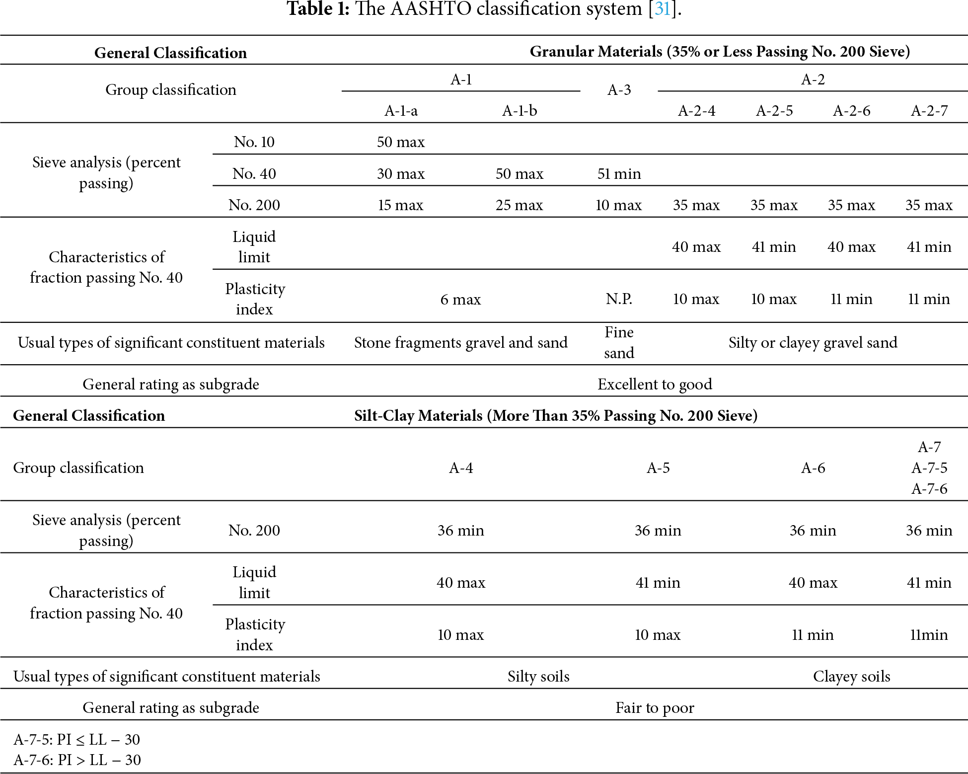
The AASHTO soil classification system provides a standardized framework for grouping soils, with widespread application in pavement and highway engineering. It was originally developed in 1929 (by C.A. Hogentogler and Karl Terzaghi) as the Public Roads Administration classification and has since undergone revisions, with the current version defined in AASHTO standard M145. Soils are assigned to one of seven primary groups, designated A-1 to A-7, using gradation characteristics together with Atterberg limit indices. Grain size distribution and plasticity are the key parameters in AASHTO classification. Atterberg limits are used to characterize the fine (silt/clay) fraction’s plasticity. In AASHTO terminology, if the portion passing No. 40 has a PI ≤ 10, the fines are deemed as silty, whereas a PI ≥ 11 indicates clayey fines. The LL of the fines is also considered, with certain groups distinguished by LL.
AASHTO classification first splits soils by how much fine material they contain. Granular materials (Groups A-1, A-2, A-3) have 35% or less passing the No. 200 sieve, whereas silt-clay materials (Groups A-4 through A-7) have more than 35% fines. AASHTO defines seven primary groups, some with subgroups, labeled A-1 to A-7. Group descriptions indicate typical soil types and their suitability as highway subgrade material. In general, A-1 soils are the best (granular, strong materials) and A-7 soils are the poorest (highly plastic clays) for supporting loads.
A-1 soils are typically well-graded mixtures of stone fragments, gravel, and sand with a small amount of non-plastic or slightly plastic fines as binder. These represent the best quality materials for subgrades, offering high stability and strength. They are subdivided into A-1-a and A-1-b. A-2 soils are a broad class of borderline granular materials. A-2 covers a variety of gravel-sand-fines mixtures that are intermediate in quality. All A-2 subgroups require 35% or less passing No. 200, but their fine fraction’s LL and PI place them in A-2-4 and A-2-5. These soils are basically sandy or gravelly materials with some non-plastic silt—still relatively good as subgrade. A-2-6 and A-2-7 have fines similar to A-6 or A-7 groups. These represent granular soils that contain a significant clay binder.
A-3 soils are chiefly fine sands, such as fine beach sand or wind-blown desert sand, with little or no silt or clay fines. They are typically poorly graded (uniform) fine sands that may contain up to about 10%–15% non-plastic silt. A-3 is basically the clean sand category: 100% passes the No. 10 sieve, and at least 51% passes No. 40. These soils still fall in the granular category and usually perform well to excellently as subgrade. A-4 soils belong to the silt-clay materials and are defined as predominantly silty soils with low plasticity. In other words, these are inorganic silt or very silty fine sand/soil. A-4 soils typically provide fair subgrade support and generally perform better than highly plastic clays; however, their behavior can degrade under wet conditions. They are commonly more compressible and exhibit lower strength than granular soils. A-5 soils are also silty materials but distinguished by having a high LL (LL > 40) while still low plasticity (PI ≤ 10). The presence of mica or diatomaceous earth can cause very high LL even with low plasticity. They are usually considered fair to poor as subgrade materials. A-6 soils are clayey soils with a substantial fine fraction that have moderate to high plasticity. These soils exhibit plastic and cohesive characteristics, though not as extreme in LL as A-7 clays. As subgrade, A-6 clays are considered fair to poor. A-7 soils are the most plastic fine-grained soils in this system, generally corresponding to high-plasticity clays or clayey silts. Because the range of plasticity is broad, A-7 is subdivided based on the relation of PI to LL. A-7-5: Soils with moderate plasticity relative to LL. They often are still highly compressible and elastic. A-7-6: Soils with high plasticity relative to LL. These are fat clays, very plastic, cohesive soils. A-7-6 materials have extremely high volume change potential and very low strength. This subgroup represents the worst subgrade soils. Both A-7-5 and A-7-6 are generally poor subgrade materials.
To further evaluate a soil’s quality as a subgrade, the AASHTO system uses a Group Index (GI). This is a numerical index that refines the classification by reflecting how marginal the soil is within its group. The higher the GI, the worse the performance expected. In geotechnical and pavement engineering, the AASHTO classification provides a quick way to judge a soil’s suitability for highway subgrade, embankment fill, or base material. Highway departments often specify acceptable soil classes for use in different layers of road construction.
In practice, AASHTO is heavily used in pavement engineering and by transportation agencies, while USCS is used in general geotechnical engineering. Each system has its own criteria, so engineers sometimes report both classifications for completeness. AASHTO emphasizes a soil’s suitability as a roadbed, using fewer broad categories, whereas USCS provides a precise description of grain size gradation and plasticity. Both require similar lab data, and both identify coarse vs. fine fractions.
AASHTO classification is determined using a combination of gradation and plasticity data. The parameters represent the essential physical and index properties required for distinguishing granular soils from fine-grained silt–clay materials, and for determining subgroup boundaries. The selected parameters and their roles are summarized as Table 2.
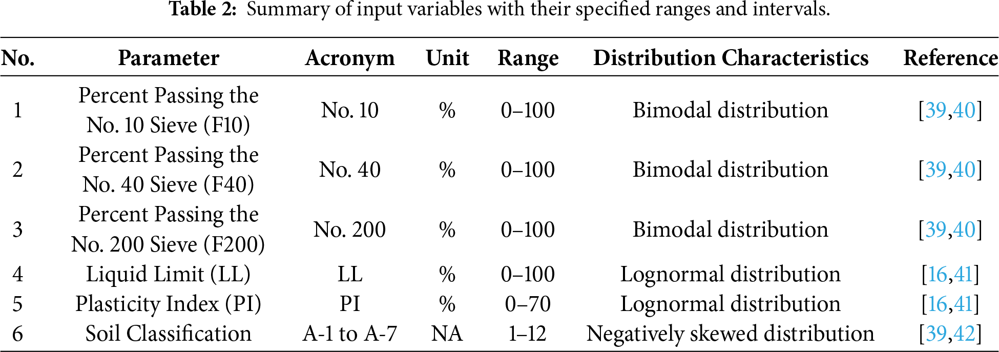
Gradation-related parameters, including the percentages passing intermediate sieves (e.g., No. 10 and No. 40), are used to distinguish among granular subgroups. These gradation characteristics affect drainage, density, and load-bearing performance, making them essential for accurate subgroup identification within the granular soil classes [32,33]. F200 represents the proportion of soil particles finer than 0.075 mm and is the most critical factor in AASHTO classification. It determines the primary division between granular soils (≤35% fines) and silt–clay soils (>35% fines). Feature-importance analysis from the RF model confirmed that F200 is the most influential variable among all inputs, exerting the strongest control on group assignment [11,34]. Liquid limit represents the moisture content at which a soil changes from plastic behavior to liquid-like flow. Within the AASHTO system, LL is used to differentiate low-plasticity soils (LL ≤ 40) from high-plasticity soils (LL > 40), particularly for identifying transitions between groups such as A-4 and A-5, and between A-6 and A-7. LL also contributes to distinguishing the two subgroups A-7-5 and A-7-6 [35,36]. PI quantifies the plasticity of the fine fraction and is a key determinant in differentiating silty and clayey behavior. Soils with PI ≤ 10 are classified as silty, whereas PI ≥ 11 indicates clayey fines. PI strongly influences subgroup boundaries within the A-2 class (e.g., A-2-4/A-2-5 vs. A-2-6/A-2-7). In the model robustness tests, omission of PI led to a notable reduction in classification accuracy, further confirming the importance of plasticity behavior in AASHTO categorization [35,37].
To ensure a comprehensive representation of AASHTO classification rules, an additional gradation feature reflecting overall coarseness to fineness distribution was included. This parameter improves model sensitivity to transitional soil types, especially within the A-2 group where mixtures of sand, gravel, and fines are common [7,38].
In the dataset construction section, a synthetic dataset was generated for model development and verification, and a supplementary dataset of 47 real-world soil samples was assembled as an application case to assess model performance under field conditions.
2.3.1 Synthetic Dataset Generation
A synthetic dataset was constructed to facilitate robust soil classification under controlled yet geotechnically realistic conditions. The input variables including the percent passing the no. 10 sieve (F10), percent passing the no. 40 sieve (F40), percent passing the no. 200 sieve (F200), LL, and PI, were sampled within parameter ranges consistent with widely used engineering standards to ensure physically plausible combinations. The resulting dataset contains 349,015 samples, organized as an input matrix of 349,015 × 5 and a corresponding output vector of 349,015 × 1 representing soil-class labels. The adoption of synthetic data is well suited to classification studies because it enables systematic coverage of the feature space, mitigates sampling bias associated with limited field and laboratory observations, and improves representation of under-sampled classes.
The synthetic dataset was generated according to the AASHTO classification rules by sampling combinations of input parameters within reasonable geotechnical ranges. Samples that violated basic physical or engineering constraints were removed to ensure engineering meaningfulness. In this way, the synthetic dataset was designed to represent plausible input conditions while preserving the rule-based AASHTO labeling logic.
Fig. 1 summarizes the marginal distributions of the five parameters and the resulting soil classes. The sieve-based fractions (F10, F40, and F200) exhibit bimodal behavior, reflecting the coexistence of soils dominated by coarse-grained depositional processes (yielding lower passing percentages) and soils enriched in fines produced by weathering and pedogenesis (yielding higher passing percentages); the overlap of these distinct grain-size populations leads to two pronounced clusters rather than a single continuous mode. In contrast, LL and PI display lognormal-like, positively skewed distributions, consistent with their dependence on multiplicative and scale-dependent controls that tend to produce asymmetric variability over a wide range. The soil classification outcomes consequently show non-uniform class frequencies, indicating that different combinations of gradation and plasticity indices occupy distinct regions of the engineering classification space.
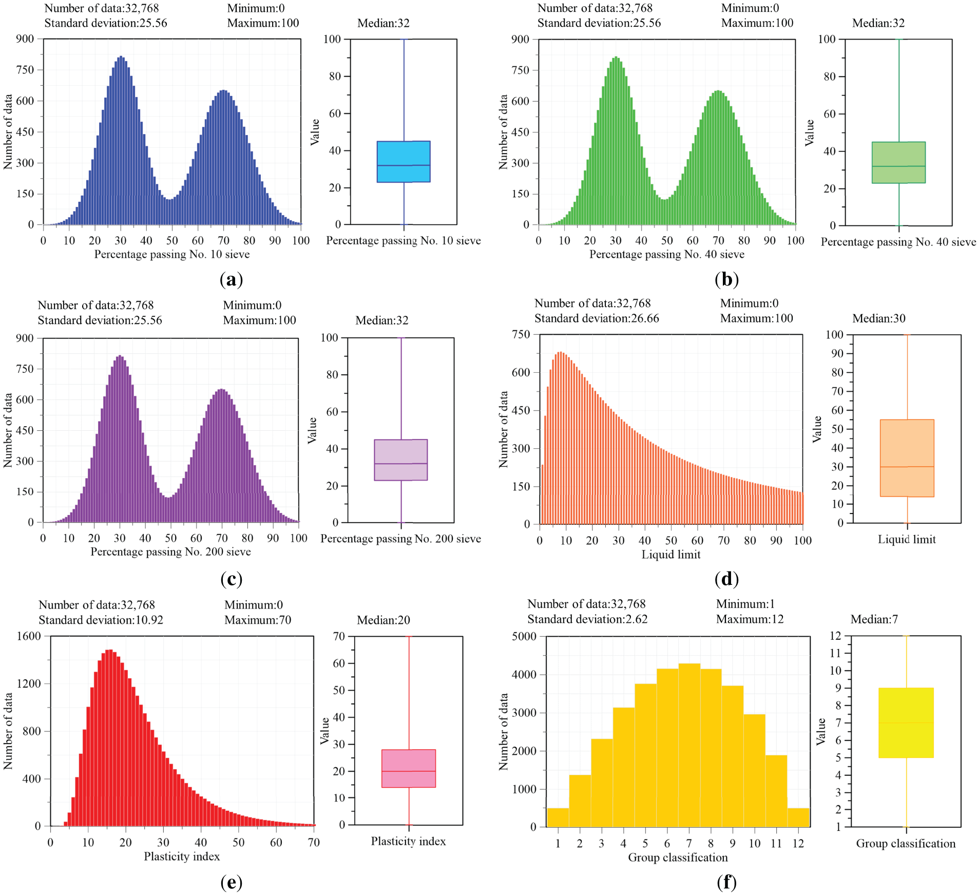
Figure 1: Distribution characteristics of parameters in the AASHTO soil classification system. (a) Percent Passing the No. 10 Sieve (F10). (b) Percent Passing the No. 40 Sieve (F40). (c) Percent Passing the No. 200 Sieve (F200). (d) Liquid Limit (LL). (e) Plasticity Index (PI). (f) Soil Classification.
Fig. 1 presents boxplots summarizing the empirical distributions of six soil-related variables across 32,768 samples, highlighting their dispersion and central tendency. The first three panels correspond to the percent passing the No. 10, No. 40, and No. 200 sieves (F10, F40, and F200). These sieve-based indices span the full range from 0 to 100 and exhibit comparable variability, with a standard deviation of 25.56 for each. The fourth and fifth panels depict the distributions of the LL and PI. LL ranges from 0 to 100 with a median of approximately 30 and a standard deviation of 26.66, whereas PI spans 0 to 70, with a median value of 20 and a standard deviation of 10.92. The final panel shows the AASHTO soil group classification number, which varies from 1 to 12 with a median of 7 and a standard deviation of 2.62.
Class imbalance could occur in synthetic data generation. To address this, the class distribution of the synthetic labels was examined by reporting/visualizing the sample counts (or proportions) for each AASHTO class. The results show that the synthetic dataset covers all soil classes and is approximately balanced. Specifically, each soil class contains more than 492 samples, indicating that class imbalance is not a major concern for the generated synthetic dataset.
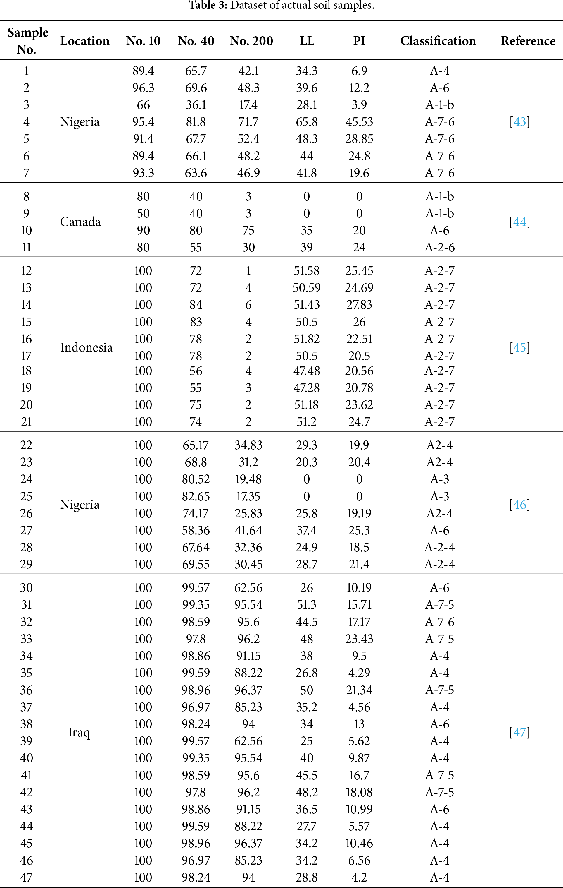
To evaluate the practical applicability of the proposed approach, a real-world soil dataset was compiled for subsequent application-case analysis. This dataset comprises 47 field samples and was employed as an independent benchmark for model validation using measured geotechnical indices and corresponding soil-class labels. Table 3 provides an overview of the dataset, reporting the sample locations, the five predictor variables used in this study, and the corresponding soil classifications. The samples were collected from multiple regions (e.g., Nigeria, Canada, Indonesia, and Iraq), representing diverse geological settings and a wide range of gradation–plasticity characteristics. This real-world soil dataset provides an independent basis for evaluating model generalizability and verifying predictive performance beyond the synthetic training set.
This study integrates AI into the AASHTO soil classification system by developing four ML models to enhance predictive classification performance. ML provides a data-driven framework capable of capturing the nonlinear and multivariate relationships among soil index properties that are often difficult to describe using conventional empirical criteria. The proposed models, RF, ANN, SVR, and DT, were selected. Model training was conducted using the synthetic dataset. To improve reliability and generalization, hyperparameter optimization and cross-validation were implemented during model development. Model performance was subsequently benchmarked through comparative evaluation, and feature-importance analyses were performed to quantify the relative contribution of individual predictors.
In this study, both a single DT and RF were included for two reasons: (1) the DT serves as a simple and interpretable baseline with low computational cost, and (2) comparing DT with RF helps quantify the performance gain achieved by the ensemble strategy for our soil-classification task. If DT performance were comparable to RF, DT would be preferable due to its simplicity and efficiency. However, our results show that RF consistently outperforms DT by a clear margin; therefore, RF was selected as the final model for soil classification.
RF, first introduced by Breiman (2001), is an ensemble learning technique that constructs a collection of decision trees and combines their outputs to enhance predictive accuracy while mitigating overfitting. Each tree is trained on a bootstrap-resampled subset of the training data, and randomness is further introduced by selecting a subset of features at each split, thereby promoting model diversity and improving generalization. Owing to its capacity to accommodate high-dimensional predictors, capture nonlinear interactions, and handle mixed-variable datasets with limited preprocessing, RF is particularly suitable for engineering classification problems. In this study, the RF classifier for the AASHTO soil classification task was formulated using hyperparameters that control model complexity and stability, including the number of trees, maximum tree depth, minimum parent size, and minimum leaf size. Hyperparameter tuning was conducted using Bayesian optimization coupled with k-fold cross-validation to ensure robust performance across the full range of input conditions. The optimal settings were identified as Minimum Parent Size = 16 and Minimum Leaf Size = 4. Fig. 2 illustrates the RF-based AASHTO classification workflow: the five soil index parameters are assembled as model inputs, and the predicted soil group is assigned based on the most frequent class output among the trees in the ensemble.
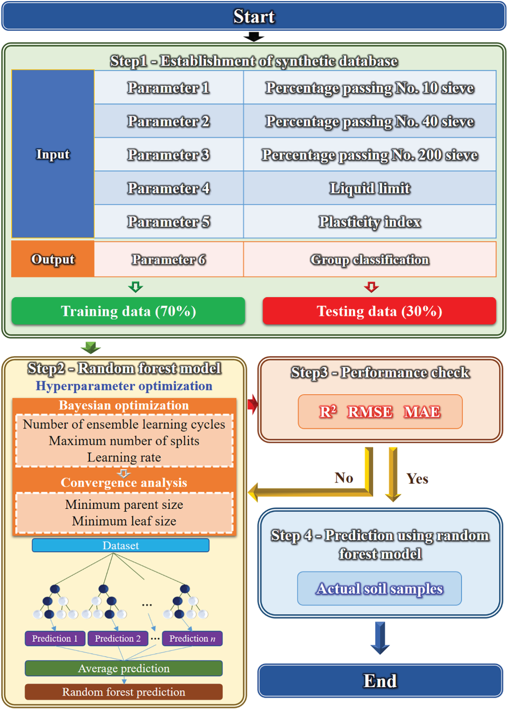
Figure 2: Flowchart of the AASHTO classification.
3.2 Artificial Neural Network (ANN)
ANNs are flexible function-approximation models designed to learn nonlinear relationships between predictors and responses. This capability is advantageous for AASHTO-based soil classification, where the governing interactions among gradation and plasticity indices are often non-additive and highly nonlinear. In this study, a feedforward multilayer ANN was employed, with the five soil indices provided to the input layer, hidden layers configured with a tunable number of neurons, and an output layer producing the predicted soil class. Nonlinearity was introduced through activation functions, and training behavior was controlled through the selection of learning rate, batch size, and initialization scheme.
3.3 Support Vector Regression (SVR)
SVR formulates prediction as a margin-based optimization problem and leverages kernel mappings to represent nonlinear input–output relationships without explicitly defining the transformation. This makes SVR well suited to geotechnical applications, where soil index variables often interact in a strongly nonlinear manner. In this study, SVR was implemented with a radial basis function kernel to accommodate complex decision boundaries. The principal tuning variables were calibrated using cross-validated grid search to improve out-of-sample performance. Because the solution is determined by a subset of training points (support vectors), SVR typically exhibits good robustness under wide parameter variability, such as that encountered in the AASHTO input space, and can be less susceptible to overfitting than some flexible nonlinear learners. Although SVR does not inherently provide direct feature-importance rankings, its stability and tolerance to noisy observations make it a competitive baseline for soil-class prediction across heterogeneous geological conditions.
Decision trees (DTs) are supervised learning models that perform classification by recursively partitioning the predictor space into increasingly homogeneous subsets, resulting in a set of hierarchical, rule-based decisions. At each split, an input variable and threshold are selected to maximize class separability by minimizing an impurity criterion. Owing to their transparent structure, DTs provide an interpretable mapping from soil index parameters (F10, F40, F200, LL, and PI) to the predicted AASHTO soil group. In this study, the DT was implemented as an AI model, with its complexity regulated by hyperparameters. These settings were tuned via cross-validation to improve generalization and reduce overfitting.
For model validation, hyperparameter optimization was performed for all four AI models to determine their respective optimal configurations. These AI models were subsequently benchmarked through a comparative performance evaluation to assess predictive capability and to identify the best-performing approach. Finally, a feature importance analysis was performed to quantify the contribution of each input variable in the AASHTO classification system and to identify the parameters that most strongly govern soil classification results.
4.1 Hyperparameter Optimization
Hyperparameter optimization was conducted for the four AI-enhanced models (RF, ANN, SVR, and DT) to determine their respective optimal configurations. The dataset was partitioned into training and testing subsets, and tuning was performed to improve robustness and reduce selection bias. Fig. 3 summarizes the tuning outcomes and convergence trends, including coefficient of determination (R2) with key hyperparameters. The optimal RF configuration was obtained at minimum leaf size = 4 and minimum parent size = 16, achieving R2 = 0.99. The ANN exhibited its best performance with 16 hidden layers and 20 neurons (R2 = 0.99). For SVR, the optimal setting occurred at kernel scale = 14 (R2 = 0.97). The DT achieved its best performance with minimum leaf size = 20 and minimum parent size = 26 (R2 = 0.91). Overall, results obtained demonstrate that the RF and ANN provided the highest predictive fidelity, indicating that ensemble- and network-based learners are particularly effective for capturing the nonlinear structure of the AASHTO classification system.
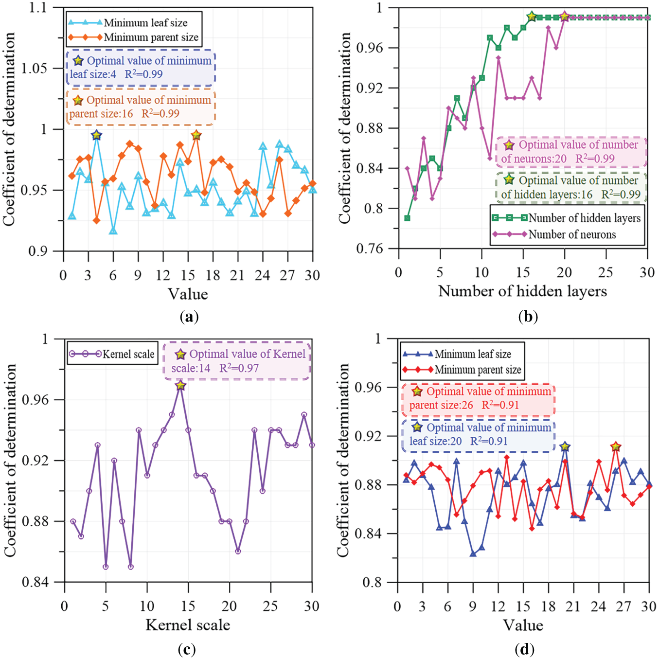
Figure 3: Results of the hyperparameter tuning using AI-enhanced models. (a) RF; (b) ANN; (c) SVR; (d) DT.
4.2 Performance of Machine Learning Models
Following hyperparameter optimization, the four AI models were implemented using their respective optimal configurations and subsequently benchmarked through a comparative evaluation to assess predictive capability and identify the best-performing approach. As summarized in Table 4, RF and ANN exhibit the strongest overall testing performance, each attaining a R2 of 0.99, indicating excellent agreement between model predictions and the observed soil classifications. RF further demonstrates the lowest prediction errors, with a root mean square error (RMSE) of 1.27 × 10⁻² and a mean absolute error (MAE) of 8.76 × 10⁻³, reflecting superior predictive precision and stability. The ANN achieves comparable goodness of fit but with slightly higher errors, with a RMSE of 2.35 × 10⁻² and a MAE of 9.54 × 10⁻³. SVR yields competitive performance, but remains inferior to RF and ANN, with a R2 of 0.97, a RMSE of 3.98 × 10⁻², and a MAE of 1.32 × 10⁻². DT presents the lowest generalization capability, with a R2 of 0.91 and the largest testing errors, including a RMSE of 6.36 × 10⁻² and a MAE of 3.04 × 10⁻². Consistent with these quantitative results, Fig. 4 shows that the regression plots for RF and ANN exhibit closer alignment between predicted and observed values, whereas larger deviations are apparent for SVR and DT. Overall, the comparative assessment confirms that RF achieves the highest prediction accuracy among the evaluated models. Accordingly, RF was selected for subsequent analyses in this study.
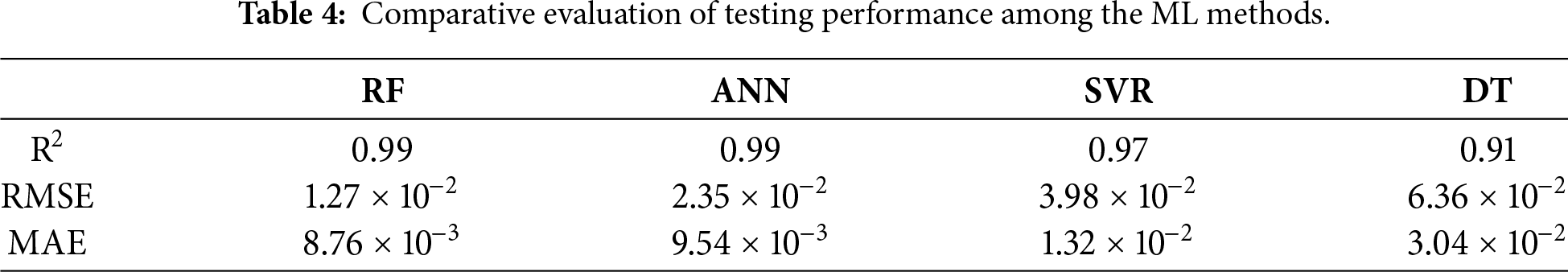
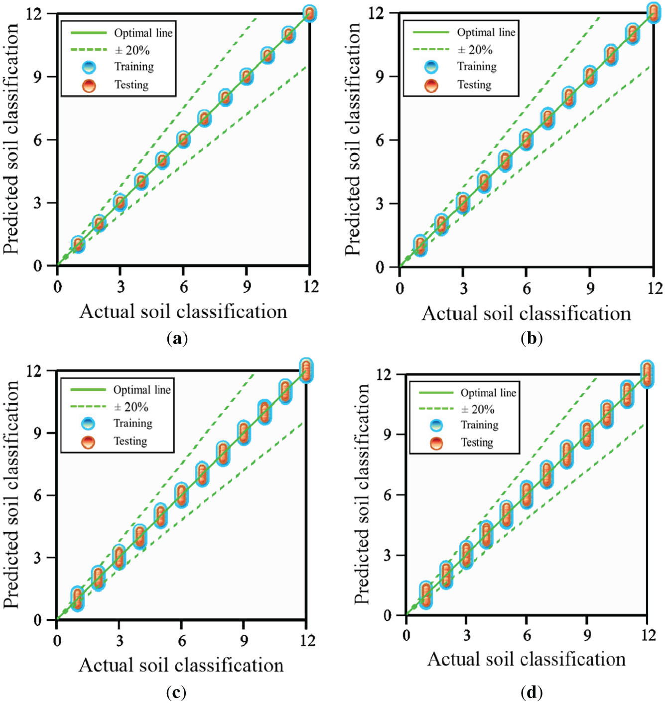
Figure 4: Performance of ML models using optimization. (a) RF model with Bayesian optimization. (b) ANN model with optimization. (c) SVR model with Bayesian optimization. (d) DT model with optimization.
Although the predictive accuracies of several models (e.g., SVC, RF, ANN) are close, this comparison remains meaningful for two main reasons. First, it provides an objective benchmark across different learning paradigms to identify a suitable model for this study. Second, because these classifiers rely on different assumptions and training mechanisms, achieving similar performance suggests that the results are not driven by a specific algorithm or overfitting, but rather reflect consistent patterns in the data. Therefore, the comparable performance across models strengthens the robustness and generalizability of our conclusions.
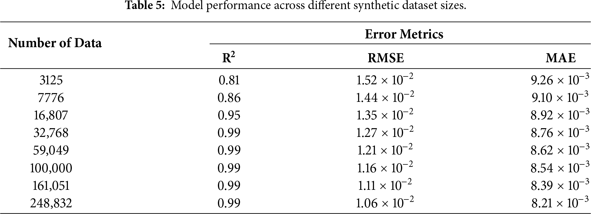
4.3 Model Performance across Different Synthetic Dataset Sizes
To examine the effect of data resolution on model reliability, this study systematically investigated model performance across synthetic datasets of increasing size. By generating databases with progressively finer parameter sampling, this analysis quantifies how expanding data volume influences predictive accuracy and error reduction, and it identifies the dataset scale at which performance stabilizes. Table 5 summarizes the model performance across different synthetic dataset sizes. The results show that the proposed model exhibits progressively improved performance with increasing synthetic dataset size. When the dataset grows from 3125 to 16,807 samples, the R2 rises from 0.81 to 0.95, while the RMSE decreases from 1.52 × 10⁻² to 1.35 × 10⁻² and the MAE decreases from 9.26 × 10⁻³ to 8.92 × 10⁻³. With 32,768 samples, the model reaches near-saturation performance with a R2 of 0.99. Further enlarging the dataset to 248,832 samples yields incremental gains, reducing the RMSE to 1.06 × 10⁻² and the MAE to 8.21 × 10⁻³, indicating improved stability and generalization from finer sampling resolution.
4.4 Feature Importance Analysis
Feature importance was assessed using the RF model to quantify the relative contribution of each input to AASHTO soil classification. As presented in Fig. 5, the importance ranking indicates pronounced differences in parameter sensitivity. Percent passing the No. 200 sieve shows the largest influence, with an importance score of 9.94, confirming that fines content is the primary control on soil group assignment in the AASHTO framework. PI is the second most influential factor, with a score of 4.92, indicating that plasticity characteristics provide substantial additional discrimination among soil groups, particularly when gradation-based indicators alone are insufficient. In contrast, the effects of percent passing the No. 40 sieve and percent passing the No. 10 sieve are comparatively smaller, with scores of 2.02 and 1.76, respectively, suggesting that these coarser gradation measures contribute to classification but play a secondary role. LL exhibits the lowest importance score of 1.23, implying a more limited incremental contribution under the current dataset. Overall, the results emphasize that fines content and plasticity dominate the predictive structure learned by the model, while the remaining gradation indices and LL exert weaker influence on classification outcomes.
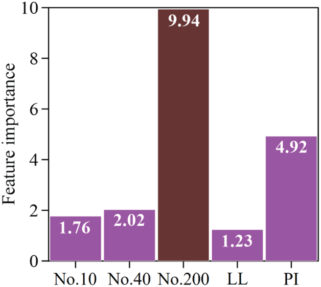
Figure 5: Importance for the factors.
To examine the practical applicability of the proposed RF approach, a real-world soil dataset was assembled for an application-oriented evaluation (Table 3), spanning multiple regions such as Nigeria, Canada, Indonesia, and Iraq. This section assesses the optimized RF model on real-world samples and examines accuracy under missing input scenarios. The models were trained primarily on the synthetic dataset to learn the AASHTO rule-consistent classification behavior. Model reliability was then evaluated using 47 real soil samples as an independent external validation set to assess generalization to measured data that include natural variability and measurement noise. Although 47 real samples are relatively limited, the purpose of using real data in this study is not to build a purely empirical model from field/lab data, but to verify that the trained models remain consistent with AASHTO classifications when applied to real-world measurements. The validation results indicate good agreement on the real samples, supporting the applicability of the proposed approach as a decision-support tool.
5.1 Validation with Real-World Data
This study examined the effects of synthetic dataset size and parameter sampling strategy on prediction accuracy. Two database construction schemes were considered: statistically distributed parameter sampling and uniform interval-based parameter sampling. Model performance was further evaluated using 47 field samples, which were used to assess prediction accuracy against real-world cases. Fig. 6 illustrates the prediction accuracy under different parameter intervals. As shown in Fig. 6, it appears that statistically distributed sampling consistently yields higher accuracy than uniform interval-based sampling. In addition, it is found that when the synthetic dataset size exceeds 32,768 samples, the prediction accuracy reaches 100%, suggesting that finer sampling resolution and larger data volume substantially improve model reliability.
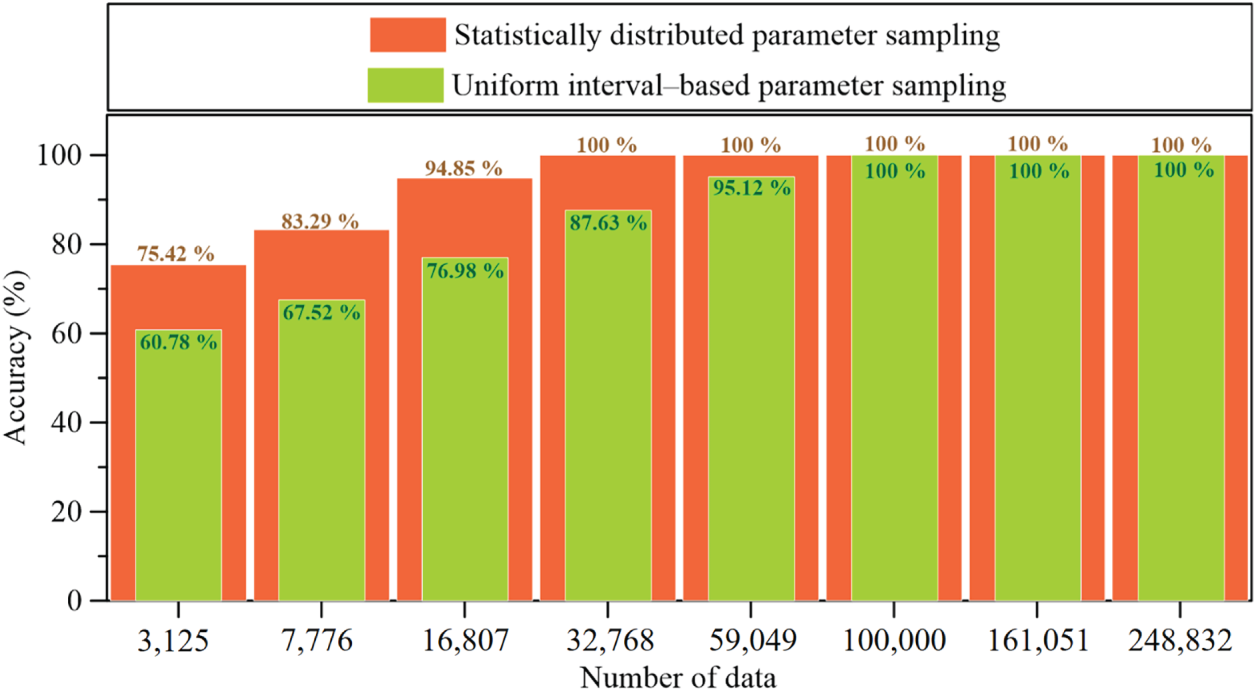
Figure 6: Prediction accuracy under different parameter interval.
5.2 Prediction Uncertainty Using Monte Carlo Simulation
Uncertainty in model predictions was assessed via Monte Carlo simulation. Using the 47 field samples, the model-derived classifications were evaluated against the corresponding observations, and a 95% confidence interval was computed for each case. Fig. 7 summarizes the results by displaying the observed values alongside the predicted mean and its uncertainty bounds; the vertical bars denote the confidence limits associated with each prediction. The analysis shows that the observed classifications are consistently contained within the 95% confidence intervals, indicating that the model predictions are statistically consistent with field measurements. Moreover, the relatively tight intervals across cases suggest limited dispersion in the simulated outputs and confirm robust predictive behavior of the proposed approach.
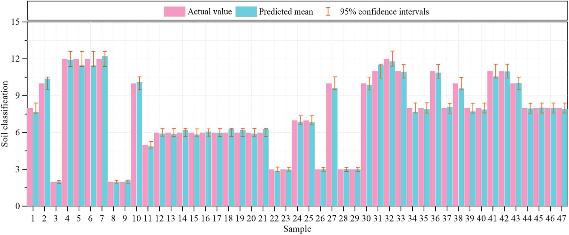
Figure 7: Monte Carlo–based estimation of prediction uncertainty for the test set.
In practical engineering applications, field or laboratory data may be incomplete, resulting in missing input parameters during rock mass classification. To evaluate model robustness under such conditions, this study investigates the predictive performance of the AI-Enhanced models when one soil classification parameter is unavailable. Missing parameters were substituted using randomly generated values to simulate the uncertainty typically encountered in real-world datasets.
To assess predictive reliability under incomplete input conditions, the missing variables were imputed using randomly generated values, and the calibrated model was used to evaluate 47 field cases. Because the stochastic imputation produces different inputs in each trial, performance was not inferred from a single run. Instead, prediction accuracy was computed as the average over multiple Monte Carlo realizations, with the number of simulations determined by convergence diagnostics. Fig. 8 shows that the estimated accuracy approaches a steady level when the number of realizations exceeds about 50. In parallel, prediction dispersion was quantified using the standard deviation across repeated runs. As illustrated in Fig. 9, the standard deviation decreases with increasing realizations and stabilizes after roughly 50 simulations, indicating convergence of the output statistics and supporting the reliability of the Monte Carlo averaging procedure.
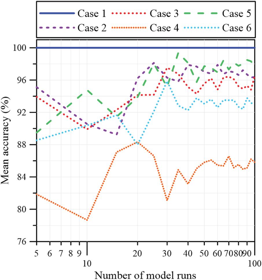
Figure 8: Convergence of mean accuracy for 100 model runs.
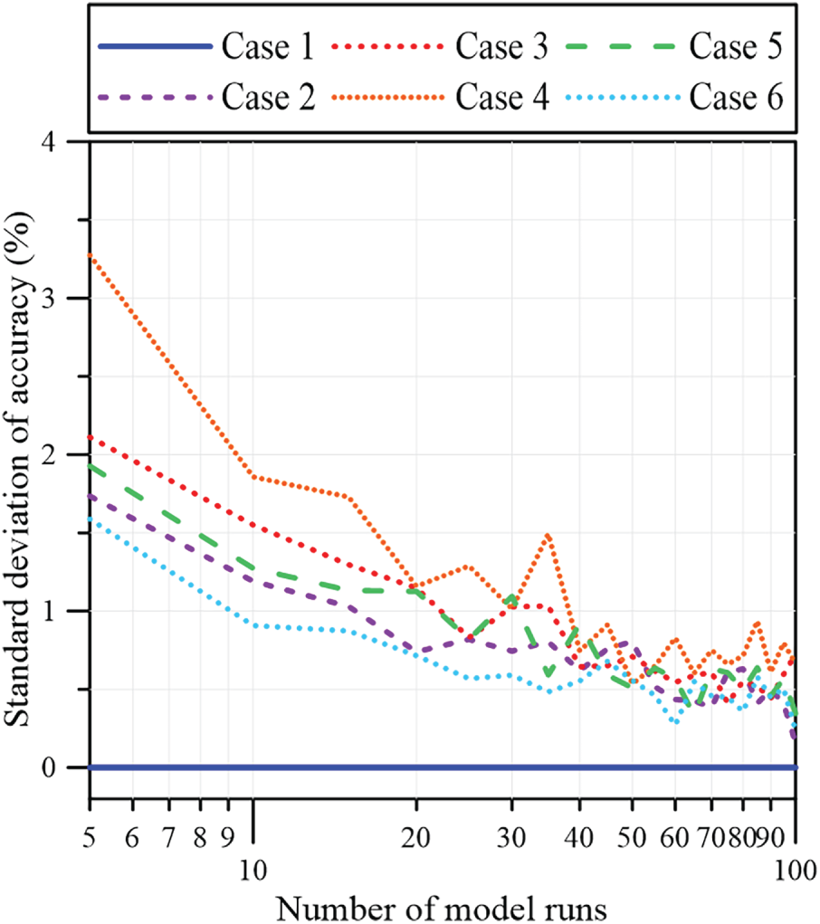
Figure 9: Convergence of standard deviation of accuracy for 100 model runs.
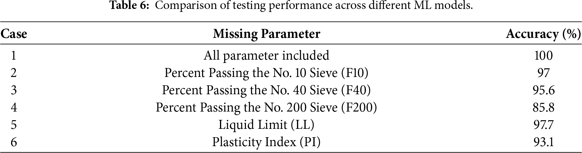
The effects on prediction accuracy, expressed as the percentage averaged over 50 runs, are summarized in Table 6. When all parameters were included, the model achieved an accuracy of 100%. However, performance declined when individual parameters were missing. The greatest decline in predictive accuracy was observed when the percent passing the no. 200 sieve was omitted, resulting in an accuracy of 85.81% and highlighting the primary influence of soil classification. Accuracy remains relatively higher when PI is missing at 93.07% and when the percentage passing the no. 40 sieve is missing at 95.57%. The smallest reductions are observed when the percent passing the no. 10 sieve is omitted, with an accuracy of 97.02%, and when LL is omitted, with an accuracy of 97.73%. Overall, the results indicate that the model is most sensitive to the absence of the percent passing the no. 200 sieve and PI, and missing either variable leads to a pronounced reduction in prediction accuracy. In contrast, the model remains relatively robust when percent passing the no. 10 sieve, percent passing the no. 40 sieve, or LL is unavailable, suggesting that these inputs have a smaller influence on classification reliability under incomplete-data conditions.
This study presents an AI-enabled AASHTO soil classification framework built on machine-learning techniques. A large synthetic database was generated from engineering consistent parameter ranges for the key AASHTO inputs, including percent passing the No. 200 sieve, LL, PI, and gradation-related indices, yielding 349,015 samples for model development. The key findings are summarized as follows:
(1) Four ML models, RF, ANN, SVR, and DT, were developed to construct an AI-based AASHTO soil classification framework. Each model was systematically tuned via hyperparameter optimization to obtain its optimal configuration. Results obtained demonstrate that RF and ANN achieve the highest goodness of fit, each attaining an R2 value of 0.99, whereas SVR yields an R2 value of 0.97 and DT attains an R2 value of 0.91. These results indicate that ensemble- and network-based models provide substantially stronger predictive capability than SVR and DT for learning the AASHTO classification system.
(2) Among the ML models, RF and ANN demonstrate the strongest consistency between predicted and reference classifications, while SVR and DT exhibit comparatively larger discrepancies. Consequently, RF is adopted as the preferred model for the AASHTO classification system due to its superior overall accuracy.
(3) Feature importance analysis indicates that percent passing the No. 200 sieve is the most influential factor, and under missing input scenarios, predictive accuracy is likewise most sensitive to the absence of this variable. These consistent findings underscore the critical role of percent passing the No. 200 sieve in the model’s performance.
(4) Uncertainty quantification via Monte Carlo simulation demonstrates that observed classifications are consistently encompassed by the 95% confidence intervals, with generally narrow bounds indicating stable and reliable predictions.
(5) Specifically, our approach is based on the AASHTO soil classification system, which was developed primarily for highway subgrade applications; thus, it may not fully capture soil behavior in broader geotechnical or engineering geology contexts (e.g., soils with similar AASHTO classes can exhibit substantially different engineering properties under the USCS). In addition, although the proposed machine learning models can perform classification under missing input scenarios, the accuracy is generally lower than that achieved with complete input parameters, and misclassification remains possible.
Acknowledgement: None.
Funding Statement: The authors received no specific funding for this study.
Author Contributions: Methodological design, experimental investigation, and manuscript preparation, Chih-Yu Liu; study conception and supervision, Cheng-Yu Ku; data management, verification, and graphical presentation, Ting-Yuan Wu. All authors reviewed and approved the final version of the manuscript.
Availability of Data and Materials: The datasets used in this study are available from the corresponding author upon reasonable request.
Ethics Approval: Not applicable.
Conflicts of Interest: The authors declare no conflicts of interest.
References
1. Palomino Ojeda JM, Quiñones Huatangari L, Cayatopa Calderón BA. Employing data mining techniques for engineering soil classification: a unified soil classification system approach. Math Model Eng Probl. 2023;10(6):1994–2002. doi:10.18280/mmep.100609. [Google Scholar] [CrossRef]
2. Ziar A. Machine learning approaches for predicting the structural number of flexible pavements based on subgrade soil properties. Sci Rep. 2025;15(1):28658. doi:10.1038/s41598-025-13852-0. [Google Scholar] [PubMed] [CrossRef]
3. Barman D, Dash SK. Stabilization of expansive soils using chemical additives: a review. J Rock Mech Geotech Eng. 2022;14(4):1319–42. doi:10.1016/j.jrmge.2022.02.011. [Google Scholar] [CrossRef]
4. Lillian N, Badawi Ahmed S, Krishnan D, Eldouma IB, Aliyu S, George OS, et al. Evaluation of sub-base material using California bearing ratio and triaxial compression tests: a case study of high court road kabale, Uganda. F1000Research. 2025;14:941. doi:10.12688/f1000research.169385.1. [Google Scholar] [CrossRef]
5. Nur SH. Shear strength behaviour of sedimentary soil stabilized by fly ash. IOP Conf Ser Earth Environ Sci. 2022;1117:012057. doi:10.1088/1755-1315/1117/1/012057. [Google Scholar] [CrossRef]
6. Balcha A, Hassen M, Geremew A, Teshome G. Engineering properties of expansive soil stabilized with barley husk ash and lime: case study of Jimma town subgrade soils. Sci Rep. 2025;15(1):41267. doi:10.1038/s41598-025-25182-2. [Google Scholar] [PubMed] [CrossRef]
7. Aydın Y, Işıkdağ Ü, Bekdaş G, Nigdeli SM, Geem ZW. Use of machine learning techniques in soil classification. Sustainability. 2023;15(3):2374. doi:10.3390/su15032374. [Google Scholar] [CrossRef]
8. Tran DT, Tran DX, Truong VH. Machine learning techniques for cohesive soil classification in construction in Vietnam. Ho Chi Minh City Open Univ J Sci Eng Technol. 2025;15(2):16–35. doi:10.46223/hcmcoujs.tech.en.15.2.3816.2025. [Google Scholar] [CrossRef]
9. O’Kelly BC. Review of recent developments and understanding of atterberg limits determinations. Geotechnics. 2021;1(1):59–75. doi:10.3390/geotechnics1010004. [Google Scholar] [CrossRef]
10. Gyasi EK, Purushotham S. Soil-MobiNet: a convolutional neural network model base soil classification to determine soil morphology and its geospatial location. Sensors. 2023;23(15):6709. doi:10.3390/s23156709. [Google Scholar] [PubMed] [CrossRef]
11. Liu CY, Ku CY, Chiu YJ, Wu TY. Evaluation of liquefaction potential in central Taiwan using random forest method. Sci Rep. 2024;14(1):27517. doi:10.1038/s41598-024-79127-2. [Google Scholar] [PubMed] [CrossRef]
12. Liu CY, Ku CY, Wu TY. Advancing rock mass classification using machine learning approach. Bull Eng Geol Environ. 2025;84(12):612. doi:10.1007/s10064-025-04585-5. [Google Scholar] [CrossRef]
13. Zhu L, Liao Q, Wang Z, Chen J, Chen Z, Bian Q, et al. Prediction of soil shear strength parameters using combined data and different machine learning models. Appl Sci. 2022;12(10):5100. doi:10.3390/app12105100. [Google Scholar] [CrossRef]
14. Khatti J, Khanmohammadi M, Fissha Y. Prediction of time-dependent bearing capacity of concrete pile in cohesive soil using optimized relevance vector machine and long short-term memory models. Sci Rep. 2024;14(1):32047. doi:10.1038/s41598-024-83784-8. [Google Scholar] [PubMed] [CrossRef]
15. Liu CY, Ku CY, Wu TY, Ku YC. An advanced soil classification method employing the random forest technique in machine learning. Appl Sci. 2024;14(16):7202. doi:10.3390/app14167202. [Google Scholar] [CrossRef]
16. Were K, Bui DT, Dick ØB, Singh BR. A comparative assessment of support vector regression, artificial neural networks, and random forests for predicting and mapping soil organic carbon stocks across an Afromontane landscape. Ecol Indic. 2015;52:394–403. doi:10.1016/j.ecolind.2014.12.028. [Google Scholar] [CrossRef]
17. Albuquerque E, Borges L, Cavalcante A, Machado S. Prediction of soil water retention curve based on physical characterization parameters using machine learning. Soils Rocks. 2022;45(3):1–13. doi:10.28927/sr.2022.000222. [Google Scholar] [CrossRef]
18. Ribeiro AJA, da Silva CAU, de Araújo Barroso SH. Neural estimation of localization and classification of soils for use in low-traffic-volume roads. Transp Res Rec J Transp Res Board. 2015;2473(1):98–106. doi:10.3141/2473-12. [Google Scholar] [CrossRef]
19. Kassa SM, Wubineh BZ. Use of machine learning to predict California bearing ratio of soils. Adv Civ Eng. 2023;2023(1):8198648. doi:10.1155/2023/8198648. [Google Scholar] [CrossRef]
20. Moreno-Maroto JM, Alonso-Azcárate J, O’Kelly BC. Review and critical examination of fine-grained soil classification systems based on plasticity. Appl Clay Sci. 2021;200:105955. doi:10.1016/j.clay.2020.105955. [Google Scholar] [CrossRef]
21. Jaffar STA, Abid MM, Khan SZ, Jafri T, Rehman ZU, Tariq MAUR, et al. Evaluation of conventional and sustainable modifiers to improve the stiffness behavior of weak sub-grade soil. Sustainability. 2022;14(5):2493. doi:10.3390/su14052493. [Google Scholar] [CrossRef]
22. Osouli A, Salam S, Tutumluer E. Effect of plasticity index and dust ratio on moisture-density and strength characteristics of aggregates. Transp Geotech. 2016;9:69–79. doi:10.1016/j.trgeo.2016.07.005. [Google Scholar] [CrossRef]
23. O’Kelly BC, Vardanega PJ, Haigh SK. Use of fall cones to determine Atterberg limits: a review. Géotechnique. 2018;68(10):843–56. doi:10.1680/jgeot.17.r.039. [Google Scholar] [CrossRef]
24. Soltani A, Azimi M, O’Kelly BC. Reappraisal of linear shrinkage test for plasticity index determination and classification of fine-grained soils. Appl Clay Sci. 2023;238:106920. doi:10.1016/j.clay.2023.106920. [Google Scholar] [CrossRef]
25. Saliba J, Al-Shaar W, Delage M. Comparison of field and laboratory tests for soil suitability assessment in raw earth construction. Appl Sci. 2025;15(4):1932. doi:10.3390/app15041932. [Google Scholar] [CrossRef]
26. Guo QM, Zhan LT, Yin ZY, Feng H, Yang GQ, Chen YM. Multi-modal fusion deep learning model for excavated soil heterogeneous data with efficient classification. Comput Geotech. 2024;175:106697. doi:10.1016/j.compgeo.2024.106697. [Google Scholar] [CrossRef]
27. Bhattacharya B, Solomatine DP. Machine learning in soil classification. Neural Netw. 2006;19(2):186–95. doi:10.1016/j.neunet.2006.01.005. [Google Scholar] [PubMed] [CrossRef]
28. Rosas DA, Burgos D, Branch Bedoya JW, Corbi A. Automatic determination of the Atterberg limits with machine learning. Dyna. 2022;89(224):34–42. doi:10.15446/dyna.v89n224.102619. [Google Scholar] [CrossRef]
29. Bian H, Sun Z, Bian J, Qu Z, Zhang J, Xu X. Assessment of soil classification based on cone penetration test data for Kaifeng area using optimized support vector machine. Sci Rep. 2025;15(1):438. doi:10.1038/s41598-024-84632-5. [Google Scholar] [PubMed] [CrossRef]
30. Zhang J, Ni J, Wang F, Huang H, Zhang D. Soil classification from cone penetration test profiles based on XGBoost. Appl Sci. 2025;16(1):280. doi:10.3390/app16010280. [Google Scholar] [CrossRef]
31. Association of State Highway and Transportation Officials. Classification of soils and soil-aggregate mixtures for highway construction purposes. Washington, DC, USA: Association of State Highway and Transportation Officials; 1993. p. 145–91. [Google Scholar]
32. Iqbal A, Farooq U, Adnan M, Ali A, Farooq U, Ullah K, et al. Effect of grain size distribution on geotechnical properties of alluvial soils. Pak J Eng Technol. 2020;3(1):31–5. [Google Scholar]
33. Chen JN, Ren X, Xu H, Zhang C, Xia L. Effects of grain size and moisture content on the strength of geogrid-reinforced sand in direct shear mode. Int J Geomech. 2022;22(4):04022006. doi:10.1061/(asce)gm.1943-5622.0002309. [Google Scholar] [CrossRef]
34. Tilahun Y, Xiao Q, Ashango AA, Dame S. Predicting resilient modulus of fine-grained soils using support vector machine-RBF and random forest. Adv Mater Sci Eng. 2025;2025(1):6503045. doi:10.1155/amse/6503045. [Google Scholar] [CrossRef]
35. Karakan E. Comparative analysis of atterberg limits, liquidity index, flow index and undrained shear strength behavior in binary clay mixtures. Appl Sci. 2022;12(17):8616. doi:10.3390/app12178616. [Google Scholar] [CrossRef]
36. Terzaghi K, Peck RB, Mesri G. Soil mechanics in engineering practice. Hoboken, NJ, USA: John Wiley & Sons, Inc.; 1996. [Google Scholar]
37. Ali Rehman M, Abd Rahman N, Rosli RN, Jusoh MNH, Sharil S, Mohd Razali SF. Relationship between plasticity index and soil erodibility: a case study of central Malaysian tropical soils. Sci Rep. 2025;15(1):40748. doi:10.1038/s41598-025-24597-1. [Google Scholar] [PubMed] [CrossRef]
38. Holtz RD, Kovacs WD, Sheahan TC. An introduction to geotechnical engineering, Vol. 733. Englewood Cliffs, NJ, USA: Prentice-Hall; 1981. [Google Scholar]
39. Das BM, Sobhan K. Principles of geotechnical engineering. 7th ed. Stamford, CT, USA: Cengage Learning; 2006. [Google Scholar]
40. Kenney TC, Lau D. Internal stability of granular filters. Can Geotech J. 1985;22(2):215–25. doi:10.1139/t85-029. [Google Scholar] [CrossRef]
41. Phoon KK, Kulhawy FH. Characterization of geotechnical variability. Can Geotech J. 1999;36(4):612–24. doi:10.1139/t99-038. [Google Scholar] [CrossRef]
42. Rada GR, Elkins GE, Hicks RG. Long-Term Pavement Performance (LTPP) program Specific Pavement Studies (SPS)-development of experiment design: SPS-11 asphalt concrete pavement preservation study (No. FHWA-HIF-18-063). Washington, DC, USA: Federal Highway Administration; 2018. [Google Scholar]
43. Alade SM. Correlation of unified and AASHTO soil classification systems for soils classification. J Earth Sci Geotech Eng. 2018;8(1):39–50. [Google Scholar]
44. Wilson G. Interpretation sheets for engineering classifications in soil surveys. Can J Soil Sci. 1983;63(4):679–89. doi:10.4141/cjss83-069. [Google Scholar] [CrossRef]
45. Khatab U, Asnur H, Yunita R. Klasifikasi tanah di Lima Kecamatan kota payakumbuh dengan sistem aashto. J Rekayasa. 2022;12(2):164–74. doi:10.37037/jrftsp.v12i2.146. [Google Scholar] [CrossRef]
46. Oghenero AE, Okey AT, Brume O, Okunuwadje SE, Jerry O. Classification and compaction characteristics of lateritic soils of Warri, Delta state. Nigeria Adv Appl Sci Res. 2014;5:451–7. [Google Scholar]
47. Al-Adhadh AR, Sakban HK, Naeem ZT. Effect of method of soil drying on Atterberg limits and soil classification. IOP Conf Ser Mater Sci Eng. 2020;739(1):012044. doi:10.1088/1757-899X/739/1/012044. [Google Scholar] [CrossRef]
Cite This Article
 Copyright © 2026 The Author(s). Published by Tech Science Press.
This work is licensed under a Creative Commons Attribution 4.0 International License , which permits unrestricted use, distribution, and reproduction in any medium, provided the original work is properly cited.
 Downloads
 Citation Tools